Impact of bot return policies in van-and-bot delivery systems

Abstract

Sidewalk Autonomous Delivery Robots (SADRs) present a promising alternative for mitigating excessive delivery traffic in smart cities. These bots operate at pedestrian speed and work in conjunction with vans to offer efficient delivery services. Existing research emphasises the development of coordinated service schedules for vans and bots to optimise customer service. In contrast, this study examines the influence of bot return policies on their travel back to designated stations after task completion. We assess three distinct return policies that dictate the station selection for bot returns and explore the relocation of bots between stations using vans. Specifically, we present a reformulation of the fleet sizing problem as a minimum cost matching problem in a bipartite graph. This reformulation allows for the efficient calculation of optimal solutions for bot fleet sizing under different return policies within polynomial time. Notably, this computational efficiency enables the analysis of large-scale cases without sacrificing the evaluation of policies with heuristic gaps. Our findings highlight the importance of carefully selecting the appropriate return policy, as the best policies have the potential to decrease the bot fleet size by up to 70%.

Keywords:

• Last-mile delivery
• autonomous bots
• return policies
• fleet sizing
• SDG9: industry
• innovation and infrastructure

1. Introduction

The continuous growth of e-commerce platforms has made home delivery services a critical backbone for efficiently supplying the population. It is, therefore, unsurprising that these delivery services, particularly on the last mile, face high expectations from various stakeholders:

• Customers: It is projected that in Germany alone, delivery companies will handle over 4.4 billion shipments by 2023. This represents a 160% increase compared to the 1.69 billion parcels delivered in 2000 (Boysen, Fedtke, and Schwerdfeger 2021). This surge in parcel volume is primarily driven by the rising sales in e-commerce. Concurrently, next-day or even same-day deliveries have become standard service offerings by most online retailers (Voccia, Campbell, and Thomas 2019). Consequently, an ever-growing number of parcels must be delivered under significant time constraints, with customers being unwilling to accept higher delivery costs, as surveys like the one conducted by Joerss et al. (2016) indicate.

• Employees: Parcel delivery often garners media attention due to its demanding work environment, characterised by stress, physical exertion, and inadequate remuneration (e.g. Peterson 2018). Moreover, many industrialised countries are grappling with an ageing population, which further strains the logistics job market (Otto and Battaïa 2017).

• General public and legislation: The escalation in delivery van usage to accommodate the steadily increasing parcel volume contributes to congestion and its detrimental effects on health, the environment, and safety, especially in urban areas (Lim, Jin, and Srai 2018). Consequently, heightened customer awareness and new governmental regulations necessitate courier services to intensify their efforts towards sustainable and environmentally friendly operations (Hu et al. 2019).

Given these challenges, last-mile logistics providers are actively seeking alternative delivery concepts to replace the traditional person-van tandems. Among these alternatives, we explore promising delivery concepts making use of Sidewalk Autonomous Delivery Robots (SADRs). The integration of SADRs into the last-mile delivery network offers numerous advantages. Firstly, their small size and low speed makes them perfectly suited for safely navigating densely populated areas, while effectively reducing both environmental impact and urban congestion. Secondly, deploying SADRs for shorter deliveries allows van drivers to concentrate on longer routes, optimising the delivery network and saving valuable time. Overall, this approach closely aligns with the expectations of the stakeholders, including customers, employees, and regulatory bodies.

1.1. SADRs and their alternative implementation concepts

In this paper, we refer to SADRs as ‘bots’ for brevity. These bots have a small load capacity, typically accommodating a single shipment at a time, and travel at pedestrian speed along sidewalks. By default, they operate in autonomous mode, but can switch to remote control if any disruptions occur. When a bot arrives at a delivery location, the customer is notified through a smartphone app, which also allows them to unlock the bot's cargo compartment and retrieve their shipment. Figure 1 illustrates three representative bot models, which are currently being evaluated in various field tests and pilot studies (see Bakach, Campbell, and Ehmke 2021; Li and Kunze 2023, for more detail).

Figure 1. SADR of Starship (left), Amazon's Scout (middle), and RoboPony of Zhenbotics (right).

From left to right, three photos depicting commercially available delivery bots: Starship, Amazon's Scout, and Zhenbotics' RoboPony.

On the one hand, due to their compact size, low weight, and reduced speed, bots are expected to cause minimal disruptions for pedestrians. On the other hand, the slower delivery speed may pose a challenge in ensuring timely deliveries. Taking these factors into account, bots have been studied in the literature within various delivery concepts:

• Launch from and return to depot: The most straightforward approach is to launch the bots from a central depot, where shipments arrive after long-haul transportation and are stored and consolidated for delivery. Note that especially large urban areas can also have multiple alternative depots to choose from Bakach, Campbell, and Ehmke (2021). Leveraging existing depot infrastructure eliminates the need for additional investments, apart from the bot fleet and associated equipment such as charging devices. Extensive research in recent years has focussed on the scheduling of bots. With the objective of creating conflict-free routes, Jun, Choi, and Lee (2022) propose two strategies for vehicle routing and conflict resolution and demonstrate how the introduced framework can help boosting bot scheduling efficiency. However, this centralised concept comes with the drawback of requiring bots to travel long distances, potentially compromising on-time deliveries and exceeding their restricted operating range.

• Launch from and return to van: To reduce the distances covered by bots, vans can carry them along with the shipments to strategic release locations (dubbed drop-off points) closer to the intended customers. After completing their deliveries, the bots return to meet with their respective vans. While onboard the van, the bots can recharge or have their batteries swapped (Yu, Puchinger, and Sun 2023), enabling them to handle multiple subsequent delivery tasks during the van's tour. Finally, all shipments loaded on board of the van are supplied, and the van and its bots return to the depot. This approach is similar to the drones-from-van concept (e.g. Agatz, Bouman, and Schmidt 2018; Murray and Chu 2015). The specific aspects of launching bots from vans are discussed in works by Chen, Demir, and Huang (2021), Chen et al. (2021), Liu et al. (2022), and Simoni, Kutanoglu, and Claudel (2020). However, bots move at pedestrian speed only. This potentially adds substantial waiting times for vans to wait for the bots to return, which is especially disadvantageous in congested city centres where parking space is scarce. A different perspective on this similar concept is presented in Mourad, Puchinger, and Woensel (2021). Their research addresses the integration of SADRs with a scheduled, underused, passenger shuttle line service to transport goods to their final destination. Bots can be transported by shuttles if the targeted delivery is not directly reachable, and the challenge of coordinating effectively the movement of robots and shuttles is addressed.

• Launch from and return to van-supplied bot station: In this concept, vans are utilised to supply shipments to bot stations, where bots are loaded with specific shipments and directly launched towards customers. After completing their deliveries, the bots return to their respective bot stations. This concept was initially proposed by Kim and Moon (2018) for drone-based parcel delivery but can also be adapted for bots (Alfandari, Ljubić, and da Silva 2022). The suitability of this approach depends on the density of the bot station network, as it either increases the bots' travel distances or requires significant investment in establishing a dense network of bot stations (Boysen, Fedtke, and Schwerdfeger 2021).

• Launch from van and return to bot station: This concept, introduced by Boysen, Schwerdfeger, and Weidinger (2018), combines elements from both previous approaches. Vans are employed to transport bots closer to customers, enabling faster delivery services. To minimise waiting times for bot returns, additional bot stations are introduced. After making a delivery, bots return to nearby bot stations, where they can recharge (Yu, Puchinger, and Sun 2023) and wait to be reloaded by vans for subsequent deliveries. The pre-positioning of bots by vans accelerates the time-critical transport leg towards customers, while the bots' unassisted travel back to the stations does not directly impact service quality. Consequently, only a sparse network of inner-city bot stations is required without compromising service (see also Boysen, Fedtke, and Schwerdfeger 2021).

Due to the advantages offered by the launch-from-van-and-return-to-bot-station (LVRS) concept, our paper focuses on exploring and analysing this particular approach.

1.2. Contributions and paper structure

This paper assesses different bot return policies for the LVRS concept. A bot return policy determines which bot station a bot should return to after completing a delivery. Specifically, we evaluate the following policies: the dedicated-station policy (where each bot is assigned to a specific station), the closest-station policy (where each bot returns to the nearest station to the last serviced customer), and the most-suitable-station policy (where bots are directed to a station that maximises operational efficiency based on service schedules). Additionally, the bot return policy governs whether bots can be relocated among stations using unused van capacity for transshipment.

Previous research on the LVRS concept (for a comprehensive survey, refer to Section 2) has mainly focussed on optimising joint service schedules for vans and bots. These studies determine truck routes along drop-off points (where bots are launched) and bot stations (where additional bots are loaded) to ensure timely delivery for a given set of customers. Some of these papers assume an abundant supply of bots at stations without explicitly considering their availability (Alfandari, Ljubić, and da Silva 2022; Boysen, Schwerdfeger, and Weidinger 2018). Others incorporate the initial bot inventory at each station to account for the actual number of available bots that can be loaded onto vans (Heimfarth, Ostermeier, and Hübner 2022; Ostermeier, Heimfarth, and Hübner 2022, 2023). However, previous research has largely neglected the bots' behaviour after completing deliveries and focussed on optimising service schedules based on fixed (or neglected) bot availabilities. In this paper, we shift the focus and optimise the bots' return behaviour to bot stations given the service schedules. This allows us to evaluate how different bot return policies impact the overall bot fleet size required to support the given service schedules. The resulting bot fleets under different bot return policies serve as critical performance measures for benchmarking the policies. In this context, our paper makes the following main contributions:

• We define three different bot return policies that determine which station each bot should return to after completing customer service, with and without the option to transship bots among stations using vans.

• We formulate the bot fleet sizing problem, which aims to determine the minimum number of bots required to fulfil given service schedules under all policies.

• We present a reformulation of the fleet sizing problem as a minimum cost matching problem in a bipartite graph, which allows to efficiently calculate optimal solutions for the bot fleet sizing problem under all policies in polynomial time. This ensures that our benchmark study of the competing bot return policies is not limited to small-scale instances and is not influenced by heuristic gaps.

• Our computational benchmark study reveals the importance of carefully selecting the bot return policy. Compared to the simplest benchmark, where each delivery job to a customer household is assigned to a dedicated bot, the most-suitable-station policy with bot transshipment leads to reductions in the bot fleet of up to 70%. In contrast, the more restrictive dedicated-station policy without bot transshipment only achieves fleet reductions of up to 16%.

The remainder of the paper is organised as follows. Section 2 provides a review of the relevant literature. In Section 3, we present a detailed problem description and outline the optimisation tasks aimed at minimising the bot fleet while servicing a given set of delivery jobs under the different bot return policies. Subsequently, in Section 4, we introduce the reformulation to a matching problem that allows to compute optimal solutions under all bot return policies in polynomial time. Using this solution approach, Section 5 presents the results of our benchmark study, comparing the different policies. Finally, Section 6 concludes the paper and discusses potential future research directions.

2. Literature review and relation to previous research

For a comprehensive overview of both novel and established delivery concepts on the last mile, as well as the operations research literature addressing these concepts, we recommend referring to the work by Boysen, Fedtke, and Schwerdfeger (2021). Further survey papers specifically dedicated to SADRs are provided by Srinivas, Ramachandiran, and Rajendran (2022) as well as Li and Kunze (2023). Since we have already introduced and discussed various delivery concepts involving SADRs, our literature review will focus on the LVRS concept examined in this paper.

Boysen, Schwerdfeger, and Weidinger (2018) were the first to optimise service schedules under the LVRS concept. They consider a scenario with a single van and multiple bots, aiming to minimise the number of late deliveries for a given set of customers with specified deadlines. They propose a decomposition heuristic that consists of a multi-start local search procedure on the first stage. This procedure determines van routes and then derives optimal bot loading and release at bot stations and drop-off points, respectively, in polynomial time on the second stage. Building upon this research, Alfandari, Ljubić, and da Silva (2022) focus on direct releases of bots from bot stations, explore alternative delay measures, and introduce a Branch-and-Benders-cut scheme to improve computational efficiency. Ostermeier, Heimfarth, and Hübner (2022) extend the problem setting by considering limited bot availability at each bot station. They also incorporate total logistics costs, encompassing both van-specific and bot-specific costs. Heimfarth, Ostermeier, and Hübner (2022) introduce a mixed van-and-bot delivery approach, where specific customers are served directly by vans while others are served by bots. Their numerical experiments demonstrate potential cost reductions of up to 43% compared to traditional truck deliveries and up to 22% compared to an LVRS system where only bots supply customers. Considering multiple parallel vans for bot releases, Ostermeier, Heimfarth, and Hübner (2023) develop a heuristic solution approach called set improvement neighbourhood search. Their computational study shows that total logistics costs can be reduced by up to 24% when considering multiple vehicles concurrently, compared to a cluster-first-route-second approach where the problem is decomposed into multiple single-van problems.

These prior studies provide valuable insights into the LVRS concept and its optimisation. However, they focus on service scheduling. In this paper, we shift the focus to the bot return policy and its impact on fleet sizing, contributing to the existing literature from a different perspective.

As already elaborated in Section 1.2, existing LVRS research on deriving service schedules either neglects the availability of bots at bot stations (Alfandari, Ljubić, and da Silva 2022; Boysen, Schwerdfeger, and Weidinger 2018) or prohibits that vans try to pick more bots up from a station than initially located there (Heimfarth, Ostermeier, and Hübner 2022; Ostermeier, Heimfarth, and Hübner 2022, 2023). We have no objections, especially against the latter approach. Since bot returns strongly depend on the customers' availability and willingness to promptly unload the bots at their doorsteps, bot returns to stations are hardly predictable. Including them into the planning of service schedules thus leads to a highly stochastic problem setup, which is hardly a stable basis to derive reliable service time windows for customers. Therefore, decomposing bot returns and involving only those bots that are definitely available, seems a valid approach for service scheduling. However, the policy governing the return of bots to stations remains critical for the success of an LVRS delivery concept.

While bot return policies have not been considered in the context of LVRS with SADRs, the return of satellite vehicles to mother ships plays a vital role in other transportation settings, such as the van-and-drone delivery system. In this context, Boysen et al. (2018) investigate the operational efficiency of three distinct return policies for drones: (A) returning to the initial take-off location, (B) returning to the next stop, and (C) unrestricted landing options. According to their findings, policy B outperforms policy A in terms of operational efficiency, with marginal differences between policies B and C. Similarly, Yang et al. (2023) focus on a model where the truck is required to wait for the drone at the launch location. This constraint adds a layer of operational rigidity not present in the standard Traveling Salesman Problem with Drones (TSP-D). On the other hand, Pugliese, Macrina, and Guerriero (2021) explore a more flexible approach where the drone can take off from a truck located either at a customer's location or at the depot but must return to the same truck after completing the delivery. Another study by Freitas, Penna, and Toffolo (2023) considers scenarios where the drone may visit a depot or rejoin the truck after completing a delivery task. Additionally, Zou et al. (2023) delve into a locker-drone delivery system optimised for community and intra-facility logistics, where drones always return to their dedicated locker after each delivery. The articles mentioned above explore various aspects of van-and-drone delivery systems, including facility location and delivery scheduling. However, none of them specifically analyse and compare different return strategies.

On the methodological front, we take a unique approach by evaluating various bot return policies from a reversed perspective, which differs from the conventional methods employed in existing LVRS research. We assume predetermined service schedules for customer deliveries and aim to minimise the fleet size of bots needed to execute these schedules feasibly. Fleet sizing for bots is a long-term decision-making task, where the specific customers to be served and the detailed service schedules of vans and bots are uncertain. We acknowledge this uncertainty but offer the following justification for our seemingly unusual problem perspective. By minimising the bot fleet size for representative service schedules, we establish an objective criterion for comparing different bot return policies. This criterion enables an assessment of the true potential of a specific policy, free from the interference of uncertainty, bounded rationality, or unrealistic small-scale instances. Our deterministic problem setup ensures this. Additionally, to address concerns related to heuristic gaps and accommodate larger problem instances, we develop an exact approach for bot fleet sizing with polynomial runtime. If a policy exhibits limited advantages under these ‘ideal’ circumstances, it is likely to be even less effective in the real world where uncertainty and bounded rationality are inevitable. Future research should build upon our initial attempt to benchmark alternative bot return policies and relax some of our assumptions.

In conclusion, bot return policies under the LVRS concept have not been previously investigated, and our study fills this research gap.

3. Problem description

This section defines our fleet sizing problem, which aims to determine the minimum number of bots required to enable the given service schedules of multiple vans operating in parallel in an urban area. The basic input for our fleet sizing problem is the set of service schedules, which are derived as follows. Initially, we have a set of customers to be serviced, drop-off points (where bots can be launched), bot stations (where vans can load bots), and a fleet of vans. Each van's service schedule is obtained using one of the optimisation approaches discussed in Section 2. In our computational study presented in Section 5, we utilise the approach proposed by Boysen, Schwerdfeger, and Weidinger (2018) to optimise the service schedules of each van, after dividing the total customer set among the vans. Note, however, that alternative solution methods described in Section 2 could also be employed. The result is a service schedule for each van, specifying the van's route along drop-off points and bot stations, as well as the loading and launching of bots and their arrival at customer homes.

From these given service schedules, we extract the bot jobs. A bot job is initiated by the loading event of some bot at a specific bot station at a specific time and includes the travel (first on the van and then autonomously) to the respective customer. The job concludes when the bot is unloaded by the customer at their home. The bot jobs, characterised by their start and end times, as well as origin and destination, serve as the fundamental input for our fleet sizing problem. For this input, we aim to determine the minimum bot fleet size that allows the feasible execution of all bot jobs. This includes ensuring that each bot is provided with the sequence of bot jobs to be performed and is informed about the bot station to approach after customer service and before being picked up by the next van. Naturally, the choice of the bot station is influenced by the adopted bot return policy.

Therefore, our problem setup involves two stages. Firstly, in Section 3.1, we explain the process of deriving the fundamental input data for our bot fleet sizing problem, which is the set of bot jobs, from the given service schedules of vans. This input is then utilised in the second stage, where the actual bot fleet sizing problem is addressed. The precise formulation of this problem can be found in Section 3.2.

3.1. Preprocessing bot jobs from service schedules

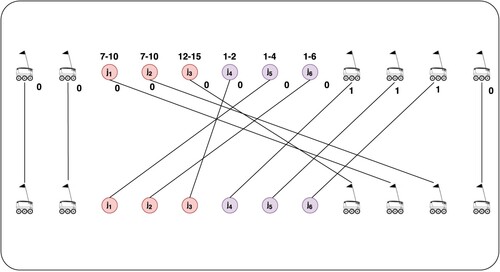
This section describes the preprocessing step to derive the bot job set, which is the basic input data to the bot fleet sizing problem defined in Section 3.2. This preprocessing task is best explained with the help of an example, such as the one depicted in Figure 2.

Figure 2. Example 1. Service schedules for two vans servicing six jobs (represented by circles). The solid-line arrows indicate the van routes, while the dotted lines depict the travel directions of the bots from the drop-off points to the final jobs. Each assigned path requires a vehicle-specific travel time, as indicated by the arc weights.

A graphical illustration mapping the service schedules of two vans (a pink van and a purple van) alongside six job locations. The van routes and bot paths feature arc weights, indicating transit times. This representation aims at showing the scheduling of jobs assigned to two different van, including their respective start and end times. In the article, this example is referred to as ‘Example 1’.

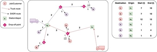
In Example 1, we have six jobs $j_1,\dots ,j_6$ (circles), four drop-off points $d_1,\dots ,d_4$ (diamonds), two bot stations $s_1$ and $s_2$ (squares), and two vans (purple and pink). Feasible service schedules for these two vans, where the pink (purple) van services job subset $\{j_1,j_2,j_3\}$ ($\{j_4,j_5,j_6\}$), are given in Figure 2. These service schedules could, for instance, be derived by first partitioning the jobs among vans and then solving the resulting single-van problems with the solution method of Boysen, Schwerdfeger, and Weidinger (2018). Recall that we follow this approach in our computational study. However, the service schedules could also be derived by the solution method of Ostermeier, Heimfarth, and Hübner (2023), where the cooperation of multiple vans is explicitly considered. From the perspective of our bot fleet sizing problem these service schedules for all vans are fixed and given.

To illustrate how the set of bot jobs, the input data for the bot fleet sizing problem, is derived from the given service schedules, we examine the service schedule of the pink van depicted in Figure 3. Assuming that the van departs from its origin at time 0, we identify three bot jobs corresponding to the performed jobs. For instance, the bot assigned to serve job $j_1$ is loaded onto the van at bot station $s_1$ when the van reaches this station at time 7. After being on board the van for a duration of 2 time units, the bot is launched at drop-off point $d_1$ and travels for an additional unit of time to reach job $j_1$. Therefore, the origin (destination) of this bot job is $s_1$ ($j_1$), and its given start (end) time is 7 (10). Note that if customers do not unload bots immediately upon arrival, this information is assumed to be known and only affects the duration of the bot's delivery job. The resulting bot jobs of the pink van are displayed on the right side of Figure 3. Together with the additional three bot jobs derived from the purple van, these bot jobs constitute the basic input data for our bot fleet sizing problem, which will be defined in the subsequent section.

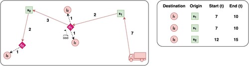
Figure 3. Example 1 (cont.). Service schedule of the pink van with three serviced jobs (left) and the set of resulting bot jobs (right).

The image provides a detailed presentation of the service schedule of the pink van in Example 1, showcasing its three serviced jobs in both graphical and tabular forms.

3.2. Definition of the bot fleet sizing problem

The preprocessing step of Section 3.1 yields the actual input data to our bot fleet sizing problem, which is a set J of bot jobs. These jobs must be feasibly serviced by some bot, such that each job's given start and end time at the origin and destination can be granted. Each job $j\in J$ is thus defined by an origin $o_j$, a destination $d_j$, a start time ${\alpha }_j$, and an end time $f_j$. On the other hand, we have a fleet B of bots to be sized.

Let $a:J\to B$ be a function that describes an assignment of jobs to bots, i.e. $a(j)=b$ means that job j is assigned to bot b. Furthermore, let ${\mathrm{\Omega }}^a=\{(j,j^{\prime }):a(j)=a(j^{\prime })\mathrm{and}{f}_j<{\alpha }_{j^{\prime }}\}$ define the set of ordered job pairs executed in direct succession by the same bot under assignment a, with j executed before $j^{\prime }$.

A solution to the bot fleet sizing problem is defined by two parts. First, we have an assignment a that matches jobs of J to bots of B. Furthermore, for any pair of bot jobs j and $j^{\prime }$ that are executed by the same bot within assignment a in direct succession, we have to define the bot station visited by the bot in between both jobs. If ${\mathrm{\Omega }}^a$ defines the set of jobs pairs $(j,j^{\prime })\in {\mathrm{\Omega }}^a$, executed in direct succession by the same bot in a, with j executed before $j^{\prime }$, then we have to define bot station $s_{j,j^{\prime }}$ for each $(j,j^{\prime })\in {\mathrm{\Omega }}^a$.

We mathematically formulate the feasibility of a solution a as follows:

• $\mathrm{\forall }j\in J,\mathrm{\exists }!b\in B:a(j)=b$: Each job $j\in J$ is successfully executed, meaning that it is assigned to exactly one bot of set B in assignment a.

• $\mathrm{\forall }(j,j^{\prime })\in {\mathrm{\Omega }}^a,{\alpha }_{j^{\prime }}\ge f_j+\delta (d_j,s_{j,j^{\prime }})$ and $s_{j,j^{\prime }}=o_{j^{\prime }}$: If two jobs are assigned to the same bot to be executed in direct succession, then there must be enough time for the bot to visit its designated bot station after job j where successor job $j^{\prime }$ starts. Thus, ${\alpha }_{j^{\prime }}\ge f_j+\delta (d_j,s_{j,j^{\prime }})$ and $s_{j,j^{\prime }}=o_{j^{\prime }}$ must hold for each $(j,j^{\prime })\in {\mathrm{\Omega }}^a$, where $\delta (o,d)$ represents the travel time of a bot from origin o to destination d.

Note that we assume that either each bot's waiting time at a bot station for the next van is long enough to be fully recharged in the meantime or batteries are swapped before a bot is loaded onto a van. This allows us to abstract from limited operating ranges of bots. However, although not explicitly considered, adding range restrictions, so that specific bot stations are beyond reach from a customer's destination, is truly straightforward.

4. Reformulation as a minimum cost bipartite matching problem

Having defined the bot fleet sizing problem, we can reframe the optimisation task as a minimum cost bipartite matching problem. This reformulation opens up the path towards exact solution algorithms with polynomial runtime. To explain this reformulation in a clear manner, we first focus on the bot fleet sizing problem under the dedicated-station policy in Section 4.1. We then proceed to discuss the necessary adjustments to the reformulation when applying the closest-station and most-suitable-station policies in Sections 4.2 and 4.3, respectively. Furthermore, in Section 4.4, we demonstrate that the reformulation requires only a few modifications to incorporate the option of transshipping bots among bot stations by utilising unused van capacity.

Note that minimising a vehicle fleet, tasked with executing a given set of time-tabled trips, through a bipartite matching has previously been explored by Bertossi, Carraresi, and Gallo (1987) to minimise bus fleets for fixed departure and return trips. Building upon this idea, we extend and adapt this approach to the bot fleet sizing problem, considering its different bot return policies.

4.1. Dedicated-station policy

Under the dedicated-station policy, each bot is assigned to a specific bot station where it is picked up by vans and returns to after customer service. Thus, bots remain at their designated bot stations, and only jobs originating from the respective bot station are considered for execution by the same bot. As a result, the overall bot fleet sizing problem can be decomposed into multiple subproblems specific to each bot station.

Example 4.1

cont.

Referring to the example introduced in Figure 2, this implies that two bot fleet sizing problems need to be solved: one for bot station $s_1$ and another for bot station $s_2$. The former problem includes jobs $J^{\prime }(s_1)=\{j_1,j_2\}$, while the latter consists of jobs $J^{\prime }(s_2)=\{j_3,\dots ,j_6\}$.

For each station-specific subproblem, we introduce a bipartite graph $G=(V,E,w)$ with a bipartition $(P,Q)$. In this context, $P=P_b\cup P_j$ and $Q=Q_b\cup Q_j$, where $P_b$ and $P_j$ are respectively the bot and job nodes in P, and $Q_b$ and $Q_j$ are respectively the bot and job nodes in Q. Additionally, P and Q are subsets of V, serving as predecessor and successor nodes, respectively. Both sets P and Q contain $|P|=|Q|=2\cdot |J^{\prime }|$ nodes.

The weights $w_e$ are associated with each edge $e\in E$ and indicate the cost or ‘penalty’ of choosing that edge in the matching.

• bot2bot: Each bot node of P is connected by an edge exclusively with one bot node of Q and vice versa. This edge represents that the respective bot is not required. This edge e is associated with an edge weight $w_e=0$, because – if realised in the matching – no additional bot is required.

• bot2job: Each bot node of P is related by an edge with any job node of Q. These edges represent that the respective job is the first one executed by a bot. All edge weights of these bot2job-edges are set to $w_e=1$, which indicates that an additional bot is utilised.

• job2job: A job node j of P is connected by an edge with a job node $j^{\prime }$ of Q, if they do not refer to the same job and ${\alpha }_{j^{\prime }}\ge f_j+\delta (d_j,\overline{s})$. Here, $\overline{s}$ refers to the bot station of the current subproblem where all delivery jobs have their origin. Such an edge represents that both jobs can be feasibly executed by the same bot, with predecessor j before successor $j^{\prime }$. The edge weights of these edges are set to $w_e=0$, because the bot already applied for the predecessor is reused by the successor.

• job2bot: Finally, any job node of P is connected by an edge with any bot node of Q. Such an edge represents that the respective job is the ultimate one executed by some bot. These edges receive edge weights $w_e=0$, as no additional bot is required.

The implementation details for the computation of the job2job edges, which determine the feasibility of executing two consecutive jobs, are given in Appendix A.3, in the case of the dedicated-station policy as well as for subsequent policies.

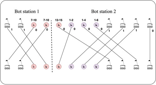
The resulting bipartite graph allows us to find a minimum cost bipartite matching, where each node in set P is matched with exactly one node in set Q, and the sum of the selected edge weights is minimised. A generic model for the resulting minimum cost assignment problem, framed within the context of our bot fleet minimisation problem, can be found in Appendix A.2. This optimisation problem can be solved in polynomial time using the well-known Hungarian method (Kuhn 1955). The method resolves the task in $O(n^3)$, where $n=2\cdot |J^{\prime }|$. The cost of the optimal solution corresponds to the minimum fleet size required to successfully execute all jobs under the dedicated-station policy. To obtain the job sequence to be executed by each bot, we start at an edge connecting a bot node of P with a job node j of Q. This is the first job of this bot. Then, we follow the chain of job2job edges of the optimal matching starting in j and so on, until finally the chain ends in a bot node of Q. The shortest chain starts and directly ends in bot nodes without intermediate job2job edges. This indicates that one of the bots, out of the initial potential fleet size determined by our upper bound, is not required.

Example 4.1

cont.

The optimal minimum cost matchings for the two matching tasks corresponding to bot stations $s_1$ and $s_2$ are illustrated in Figure 4. In the case of bot station $s_2$, the solution indicates that one bot starts with job $j_4$, then, after temporarily returning to $s_2$, it proceeds to execute job $j_3$, which is its final task. This particular bot performs two jobs, resulting in the elimination of one bot. The other two bots only execute jobs $j_5$ and $j_6$, respectively. Hence, the bot fleet size required for station $s_2$ amounts to three. Along with the two additional bots necessary for $s_1$, the total bot fleet size under the dedicated-station policy is $|B|=5$.

Figure 4. Optimal solutions for Example 1 under the dedicated-station policy with node set P (resp. Q) in the upper (resp. lower) part of the figure. The instance decomposes into two minimum cost bipartite matching subproblems. The total minimum fleet size results to $|B|=5$.

The figure graphically illustrates the reformulation as a minimum cost bipartite matching problem, depicting the respective assignments in the case of an optimal solution under the dedicated-station policy. It clearly demonstrates the separation of Example 1 into two subproblems, one for each bot station.

Note that the bot nodes do not need to be included in the node sets P and Q. In such a case, it is sufficient to determine a perfect matching in the bipartite graph, where the initial jobs assigned to bots are those without any predecessors in their respective job chains. The number of chains then equals the minimum fleet size. More detailed information on this approach can be found in works such as Boysen and Emde (2014). However, we chose to include these bot nodes and employ a minimum cost bipartite matching, as it allows for a clearer description of our approach without compromising its solvability in polynomial time.

4.2. Closest-station policy

Under the closest-station policy, it may occur that a bot is picked up from one bot station to service a specific customer but returns from there to a different station, which is closer to the last customer. With bots (potentially) changing their bot stations, the bot fleet sizing problem no longer decomposes into single-station subproblems. Thus, we have one unique graph $G=(V,E,w)$ under this bot return policy, where bipartition $(P,Q)$ receives $|P|=|Q|=2\cdot |J|$ nodes as defined above, i.e. $|J|$ bot nodes and another $|J|$ job nodes. The only other alteration arises for the job2job edges. They are inserted between a predecessor job $j\in P$ and a successor job $j^{\prime }\in Q$, only if ${\overline{s}}_j=o_{j^{\prime }}$, where ${\overline{s}}_j$ refers to the bot station being closest to customer j, and ${\alpha }_{j^{\prime }}\ge f_j+\delta (d_j,{\overline{s}}_j)$ holds. The weights of these edges are still set to $w_e=0$.

Example 4.1

cont.

In our example, under the closest-station policy, we observe that the bot that serviced job $j_6$ does not return to its original bot station $s_2$. Instead, it takes a one-time unit to drive to the closer bot station $s_1$. From there, the bot is picked up to serve job $j_2$, resulting in a saving of a bot compared to the previous solution under the dedicated-station policy. Figure 5 illustrates an optimal minimum cost bipartite matching, which yields a fleet size of $|B|=4$ bots.

Figure 5. Optimal solution to Example 1 under the closest-station policy with a resulting minimum fleet size of $|B|=4$.

The figure graphically illustrates the reformulation as a minimum cost bipartite matching problem, showcasing the respective assignments in the case of an optimal solution under the closest-station policy.

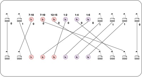
4.3. Most-suitable-station policy

The most-suitable-station policy offers bots even more flexibility to switch between bot stations. Therefore, just as for the closest-station policy, the problem does not decompose into station-specific subproblems. We have one unique graph $G=(V,E,w)$, whereby bipartition $(P,Q)$ still receives $|P|=|Q|=2\cdot |J|$ nodes as defined above. Again, only the generation rule for the job2job edges alters. They are inserted between a predecessor job $j\in P$ and a successor job $j^{\prime }\in Q$, whenever ${\alpha }_{j^{\prime }}\ge f_j+\delta (d_j,o_{j^{\prime }})$ holds. The weights of these job2job edges are still set to $w_e=0$.

Example 4.1

cont.

In the case of Example 1, the most-suitable-station policy reduces the required bot fleet to three, as shown in the optimal matching presented in Figure 6. This reduction is achieved by a bot that, after serving bot job $j_5$, does not return to the closer station $s_2$ but instead moves towards $s_1$. This movement, assumed to take 3 time units, enables this bot to be loaded onto the pink van to service job $j_1$.

Figure 6. Optimal solution to Example 1 under the most-suitable-station policy with a resulting minimum fleet size of $|B|=3$.

The figure visually illustrates the reformulation as a minimum cost bipartite matching problem, depicting the respective assignments in the case of an optimal solution under the most-suitable-station policy.

4.4. Transshipment of bots among stations by vans

When executing a given service schedule, it can happen that the number of bots (equal to the number of customers serviced on the way towards the next station), while a van moves from one station to the next one, is less than the bot-carrying capacity of the van. In such cases, the available space inside the van can be utilised to transship bots from one station to the next if there are requests for new bots at the destination station. Naturally, potential bot relocations can only occur when the closest-station or most-suitable-station policies are implemented. The dedicated-station policy, on the other hand, assigns bots to specific stations, making relocations inconsistent with this approach.

Example 4.2

Displayed in Figure 7, illustrates this new feature for service schedules involving three vans (blue, black, and orange). The blue van executes delivery job $j_2$ originating from bot station $s_1$, with starting time ${\alpha }_2=3$ and end time $f_2=6$. The bot assigned to this job uses one spot of the blue van's bot-carrying capacity. If this capacity, however, is more than one, then the blue van can carry additional bots on board during its drive from station $s_1$ at departure time 3 to $s_2$ at arrival time 7, and relocate bots between these two stations.

Figure 7. Example 2 with bot relocation. Left: Given service plan with three van tours. Right: Optimal matching solution with a resulting minimum fleet size of $|B|=2$.

The figure introduces ‘Example 2’, demonstrating a scenario where vans are allowed to relocate bots between stations. The figure is divided into two parts: the left side illustrates the paths of vans and bots during delivery and relocation, while the the right side presents the classical bipartite graph with the addition of relocation nodes.

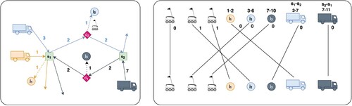
To account for bot relocations in our bipartite matching approach, we additionally introduce relocation nodes into both partitions P and Q of our bipartite graph $G=(V,E,w)$. For each van drive connecting two bot stations (including potential intermediate stops at drop-off points), we introduce a relocation node for each unused bot capacity unit on board of a van.

We assume that all three vans in Example 2 have a capacity of boarding up to two bots. On its drive from station $s_1$ to $s_2$, one of the available two slots in the blue van is already taken by the bot dedicated to servicing job $j_2$. Similarly, the black van has one available free slot when driving from station $s_2$ to $s_1$. We introduce thus two relocation nodes into both P and Q (indicated by the van icons in Figure 7, right side).

The relocation nodes are connected to other nodes by the following edges:

• bot2relocation and relocation2bot: It is unnecessary to connect bot nodes of P with relocation nodes of Q and vice versa. The scenario where bots start their service directly at the destination of the respective van drive cannot result in a worse solution compared to starting service with an unproductive drive ending at the same station. Similarly, adding a final van drive to the chain of a bot cannot improve the solution. Hence, these edges are omitted in the graph.

• relocation2relocation: A relocation node of P is connected with exactly one relocation node of Q (and vice versa). Such an edge represents the situation in which a van's available bot-carrying space is not utilised for a given drive between two stations.

• job2relocation and relocation2job: An edge is added from a relocation node of P to a job node of Q (and vice versa) if the time span between the given end time of the predecessor and the start time of the successor allows the bot enough time to drive from the destination of the predecessor to the origin of the successor.

All edges related with relocation nodes receive weight $w_e=0$, as no additional bot is involved, whether available relocation capacity of vans is utilised or not.

The optimal minimum-cost bipartite matching for Example 2 is shown on the right side of Figure 7. In this matching, two bots are required. After servicing job $j_1$, the selected bot returns to $s_1$ early enough to board the blue van for the drive from $s_1$ to $s_2$. Upon reaching $s_2$, the bot arrives on time to be loaded onto the black van and subsequently service job $j_3$.

5. Experiments and results

Our bot fleet sizing problem, under all bot return policies, can be solved to proven optimality in polynomial time (see Section 4). Therefore, even instances with hundreds of bot jobs can be solved within a few seconds. As a result, we do not evaluate the computational performance of our solution approach and instead focus on benchmarking the bot return policies. To accomplish this, we describe the experimental framework and instance generation process in Section 5.1 and present the results of our benchmark study in Section 5.2.

5.1. Experimental framework

The primary input data for our bot fleet sizing problem consists of the given service schedules for vans and bots during customer servicing. Each van is assigned a set of customers to serve. The route includes depots and drop-off points where SADRs are deployed to deliver parcels to the final customers. To obtain these schedules, we utilise the instances provided by Boysen, Schwerdfeger, and Weidinger (2018) and solve them using the algorithm introduced by the same authors. This process results in single-van service schedules where a subset of customers is served by bots that are picked up and released by the same van. In practical settings, there is often a requirement to coordinate overlapping delivery schedules in the same area while serving multiple customers concurrently. To address this complexity, our study encompasses these scenarios, allowing for the reuse of delivery bots across different van schedules. This broader perspective enhances the model's applicability to real-world situations.

The instances of Boysen, Schwerdfeger, and Weidinger (2018) are categorised into two types: small (urban) and large (suburban) instances. Table 1 presents the characteristics of these instances, including their dimensions, the number of available bot stations, drop-off points, and customers, as well as the bot capacity on board of vans. Note that these instances presuppose an average travel speed of 30 km/h and 5 km/h of van and bot, respectively. They are, then, solved with the decomposition heuristic introduced by Boysen, Schwerdfeger, and Weidinger (2018) (for more detail, see Section 2). Examples of the resulting single-van service schedules are shown in Figure 8, where we use solid red arrows to represent the van route and dashed green lines to indicate the vans' ideal trajectory from the release point to the assigned job position.

Figure 8. Single-van service schedules for the small (left) and large (right) instances.

In this figure, two instances are illustrated. On the left side, a depiction of a small instance is presented, providing visibility into the paths of both the van and the bots. On the right side, a larger instance is showcased, highlighting the complexity associated with handling larger instances due to the substantial number of available jobs.

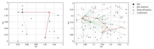
Table 1. Characteristics of the service scheduling instances of Boysen, Schwerdfeger, and Weidinger (2018).

	Small (urban)	Large (suburban)
Area	$2\mathrm{km}\times 2\mathrm{km}$	$5\mathrm{km}\times 5\mathrm{km}$
Number of bot stations	4	16
Number of drop-off points	6	30
Number of customers	6	40
Bot-carrying capacity of vans	2	8

Expanding upon these initial single-van service schedules, we broaden our analysis by concurrently executing multiple schedules within a given planning horizon, such as an entire delivery day within a specific area. Table 2 provides insights into various metrics relevant to different instance classes in our bot fleet sizing problem. Specifically, the table itemises the number of single-van delivery schedules, each tailored to serve a unique subset of customers. It also categorises the different types of service scheduling instances and enumerates the total bot jobs generated by these schedules.

Table 2. Generated instances types for the bot fleet sizing problem.

Type	Service schedules	Environment	# of bot jobs
u_4	4	urban	24
u_8	8	urban	48
u_16	16	urban	96
u_32	32	urban	192
u_64	64	urban	384
s_4	4	suburban	160
s_8	8	suburban	320
s_16	16	suburban	640

To create a realistic scenario, we merge various service schedules from the original instances, emphasising customer sets within the same geographic area where multiple vans are in operation. This consolidation provides a realistic representation similar to actual urban and suburban delivery settings, where multiple vans follow distinct schedules to deliver packages to end customers. This approach allows us to evaluate different policies regarding the reuse of bots by testing them across the entirety of the newly generated consolidated instances.

On a typical delivery day, multiple concurrent delivery schedules operate within the same area, each serving a specific subset of customers. Considering this context, we assess these instance types across different planning horizons by varying the start time intervals for van service schedules. These intervals are set at 0, 30, 60, 90, and 120 minutes. Within each interval, vans depart at equidistant start times, ensuring a distributed coverage similar to realistic delivery planning scenarios.

For each of the interval configurations, we generate 100 distinct instances of the bot fleet sizing problem and evaluate them using all five bot return policies. This approach results in a total of 20, 000 solution runs, providing a comprehensive dataset that accounts for various real-world operational conditions.

5.2. Computational results

Our computational benchmark study compares the following bot return policies: the dedicated-station policy (each bot is assigned to a fixed station to return to after customer service), the closest-station policy (each bot returns to the station closest to the last customer), and the most-suitable-station policy (bots are directed to a station where they can be reused for further jobs based on the given service schedules). The latter two policies are investigated with and without the option to transship bots among stations by utilising unused van capacity. Our evaluation criterion for the resulting five policies is their respective bot fleet sizes required to feasibly execute the given service schedules.

Table 3 provides a summary of the results obtained from this benchmark test. In this table, we report the percentage savings in the bot fleet size achieved by each policy relative to the most basic policy, referred to as the one-job-one-bot policy. Here, each job is executed by its own bot. Column ‘Reloc.’ indicates whether (+) the respective policy allows bot relocations by van or not (−). The savings are specified for the different types of instances (i.e. ‘u_4’, ‘u_8’, ‘u_16’,‘u_32’, ‘u_64’, ‘s_4’, ‘s_8’, and ‘s_16’) and for different intervals (column ‘Int.’) used to determine the start times of the vans' service schedules. Based on these results, the following findings can be observed:

Table 3. Reduction of bot fleet size in % in relation to the one-job-one-bot policy.

Int.	Policy	Reloc.	u_4	u_8	u_16	u_32	u_64	s_4	s_8	s_16
0	dedicated	–	0.3	0.6	0.9	1.4	1.7	<0.1	0.1	0.1
	closest	–	0.3	0.6	0.9	1.4	1.7	<0.1	0.1	0.1
	most-suitable	–	0.3	0.5	0.7	1.1	1.2	<0.1	0.1	0.1
	closest	+	0.3	0.6	0.9	1.4	1.7	<0.1	0.1	0.1
	most-suitable	+	0.3	0.6	0.7	1.1	1.2	<0.1	0.1	0.1
30	dedicated	–	7.5	11.8	13.2	13.6	14.0	0.6	1.2	1.9
	closest	–	9.5	13.9	14.3	14.2	14.4	0.9	1.6	2.2
	most-suitable	–	11.1	15.9	19.2	22.9	26.3	1.0	1.7	2.3
	closest	+	10.5	15.3	15.3	14.7	14.6	1.0	1.8	2.3
	most-suitable	+	12.1	17.1	20.2	23.4	26.6	1.11	1.9	2.4
60	dedicated	–	10.7	14.8	15.1	15.5	15.4	1.3	2.1	2.5
	closest	–	13.5	17.3	16.4	16.2	15.9	2.2	2.8	3.0
	most-suitable	–	24.9	33.8	40.2	45.8	50.6	3.1	4.9	7.0
	closest	+	15.2	19.1	17.4	16.7	16.1	2.5	3.1	3.2
	most-suitable	+	26.5	35.4	41.2	46.3	50.9	3.6	5.2	7.2
90	dedicated	–	11.7	15.7	15.7	16.2	16.0	1.7	2.4	2.8
	closest	–	14.7	18.5	17.1	16.9	16.5	2.8	3.3	3.4
	most-suitable	–	38.0	46.7	53.6	58.7	63.3	6.7	10.3	15.2
	closest	+	16.6	20.2	18.1	17.3	16.7	3.2	3.6	3.5
	most-suitable	+	39.7	48.4	54.6	59.3	63.6	7.1	10.5	15.4
120	dedicated	–	12.1	16.4	16.1	16.5	16.4	1.8	2.6	2.9
	closest	–	14.9	19.0	17.6	17.3	16.8	3.2	3.6	3.6
	most-suitable	–	46.7	55.2	61.5	66.2	70.4	10.9	16.8	23.9
	closest	+	16.8	20.8	18.5	17.8	17.0	3.5	3.9	3.7
	most-suitable	+	48.1	56.9	62.4	66.7	70.7	11.3	17.1	24.0

Finding 1: No significant difference between the dedicated-station and the closest-station policy. Among our various instance types and start time intervals, the difference of the average improvement over the baseline policy is just 0.9% on average and at most 3.0%. Both policies are easy to implement, but from an organisational standpoint, the dedicated-station policy provides a more stable environment. If a fixed bot fleet is assigned to each station, the capacity and charging equipment can be appropriately dimensioned, avoiding unexpected shortages when an unexpectedly high number of bots chooses a particular (closest) station. Therefore, if only being left the choice among these two policies, our results suggest that the dedicated-station policy induces no significant performance loss.

Finding 2: The most-suitable-station policy clearly outperforms its competitors. The most-suitable-station policy offers fleet size reductions of up to 70%, while the dedicated-station and closest-station policies only enable reductions well below 20%, even under optimal conditions. Therefore, directing bots to the most suitable stations is unequivocally the best policy choice, as it ensures substantial fleet reductions in the majority of scenarios.

Finding 3: Relocating bots between stations by van does not yield significant benefits. When comparing the closest-station and the most-suitable-station policy with and without the option to relocate bots by van, we record that the average improvement is just 0.6% and at most 1.9%. These marginal additional savings hardly justify the added organisational complexity introduced by a bot transshipment process.

Finding 4: The savings decrease in the suburban environment where the bot stations and customers are located at a greater distance from each other. When comparing the reductions in bot fleet size between urban instances (indicated by the prefix ‘u’ within Table 3) and suburban instances (indicated by the prefix ‘s’), we observe that the reductions in the bot fleet size are much smaller for all policies in the suburban environment. In the suburban setting, bot stations and customers are farther apart, resulting in long travel times for the bots when switching to another station. This reduced flexibility leads us to conclude that the bot return policy is more mission critical in the urban context.

Finding 5: The savings increase when the delivery dates are more evenly distributed throughout the day. If all vans start their service schedules at the same time (service time interval ‘Int.’ of length 0 within Table 3), this implies that most bots are utilised simultaneously. As a result, there is limited opportunity to reuse a bot for subsequent jobs, and the bot fleet reductions of all policies, compared to the one-job-one-bot baseline policy, never reach 2%. However, if the vans depart within a start time interval of 120 minutes, the first bots have already returned and can be reused for subsequent jobs. In this scenario, all policies achieve substantial reductions of more than 10%, except in the suburban environment where only the most-suitable-station policies reach these figures. We conclude that a logistics service provider offering SADR services requires a large bot fleet if all customers expect delivery (almost) at the same time. Therefore, all organisational measures should be evaluated to level the delivery dates of customers throughout the day. For instance, price discounts could be offered if customers accept later deliveries.

Finally, it is important to provide some perspective on our findings and acknowledge the limitations of our study. Firstly, the significant fleet reductions achieved by the most-suitable-station policy, up to 70% compared to the one-job-one-bot policy, may not be attainable when service schedules are uncertain. Forecast errors regarding the regional distribution of demand can reduce the savings in such cases. However, our results highlight the potential benefits if forecast accuracy can be improved to provide bots with accurate information on the right stations to return to. Since many jobs require preparation time before shipment (such as the picking of ordered products from a distribution centre or cooking the ordered meals), future customers to be serviced are often known when selecting return stations, although detailed service schedules may not be available. If this information can be effectively utilised within reliable forecasts, our results suggest that substantial gains can be achieved. Secondly, the limited performance improvements observed with bot transshipment are specific to our experimental setup. In different environments (e.g. within a sparse network of bot stations where limited operating ranges restrict flexibility or only limited charging infrastructure is available or if there is a significant shift in demand among regions throughout the day) higher gains may be possible.

Overall, our findings represent an initial attempt to evaluate bot return policies and reveal a significant potential for improvement when applying SADRs. Moreover, our methodology is directly applicable to multi-period delivery plans, for which return policies require accomodating extended time frames and service interruption. A comprehensive discussion on these aspects can be found in Appendix A.1.

6. Conclusion

In the context of last-mile delivery, this paper investigates a delivery concept where vans pick up small delivery bots from bot stations and transport them to drop-off points closer to the customers. The bots then handle the final leg of the delivery and, after serving the customers, return to the bot stations for the next pickup. In our study, we examine different bot return policies that regulate how bots are assigned to bot stations over time. Specifically, we investigate the following bot return policies: the dedicated-station policy (each bot is assigned a specific station), the closest-station policy (each bot returns to the bot station nearest to the last customer), and the most-suitable-station policy (bots are directed to a station where they can be efficiently reused for additional jobs based on the given service schedules). We analyse the latter two policies with and without the option to transship bots among stations by utilising unused van capacity. To assess the impact of these five bot return policies on the bot fleet size, we formulate an optimisation problem where the objective is to minimise the fleet size under each policy while ensuring the feasibility of the given service schedules for customers. We demonstrate that this bot fleet sizing problem can be reformulated as a minimum cost bipartite matching problem, which allows for polynomial-time solutions with proven optimality. In our computational study, we benchmark the bot return policies and provide managerial advice on how to effectively apply them. Our research highlights the crucial importance of return policy selection in optimising bot logistics. Notably, the most-suitable-station policy has the potential to significantly reduce fleet size, by as much as 70%, distinguishing it from seemingly comparable options like the dedicated-station and closest-station policies. Additionally, it is essential for stakeholders to recognise that the effectiveness of bot return policies faces significant constraints in suburban environments, contrasting sharply with urban contexts. Another key takeaway is the significance of timing; distributing delivery schedules throughout the day can significantly enhance efficiency across all policy types, with the most-suitable-station policy showing the greatest benefit. These findings provide stakeholders with valuable insights for tailoring bot return policies and operational strategies, enabling more effective resource allocation and improved logistical planning, especially when operating across diverse geographic landscapes. Future research could build upon these findings, exploring the implications of potential technological advancements for the bots and methodological enhancements to our approach. Enhancing the battery capacity and/or top speed of the bots could significantly improve the overall system, enabling them to reach stations located farther within the service area. Particularly, the development of longer-lasting battery technologies would extend the operational range before requiring recharging. Given the ongoing development of multi-container, higher-capacity bots capable of carrying more than one parcel, this would open the door for bots to deliver multiple parcels before needing to return to a station. While our current study assumes a priori knowledge of delivery plans, future work could address this limitation by incorporating uncertainty into service schedules. This would enable a more thorough examination of different bot return policies under non-deterministic conditions. Additionally, evaluating alternative performance measures beyond bot fleet size could provide a more comprehensive understanding of how return policies impact the performance, reliability, and client satisfaction of a last-mile delivery concept that includes delivery bots. Finally, our study considers bot fleets that can be operated by a single entity. Without being restricted to situations arising within a single company, our framework could be extended to multiple firms operating in the same area. Allowing for bot exchangeability between firms would facilitate further minimisation of the global number of devices in use, as well as the number of available bot stations in the serviced area. However, further research would be necessary to analyse the conditions under which such a cooperative framework could be successfully implemented.

Disclosure statement

No potential conflict of interest was reported by the author(s).

Data availability statement

The data that support the findings of this study are available from the corresponding author, M.G., upon reasonable request.

Additional information

Notes on contributors

Mikele Gajda

Mikele Gajda is a PhD student at HEC Lausanne, the business school of the University of Lausanne. He holds a master's degree in computer science and engineering from the University of Brescia with a thesis in combinatorial optimisation in collaboration with the Management Department of the Technical University of Denmark (DTU), where he spent an academic semester. His research focuses on developing optimisation algorithms for transportation and logistics problems, using both exact and heuristics algorithms to tackle complex real-world applications.

Nils Boysen

Nils Boysen is Professor of Operations Management at the Friedrich-Schiller-University of Jena (Germany). He received a Diploma Degree and a PhD in Business Administration from the University of Hamburg. Before that, he worked for IBM Global Services. His main research interests are logistics, operations management, and optimisation techniques.

Olivier Gallay

Olivier Gallay is a full professor of operations research at the University of Lausanne. His current research interests include supply chains operations, sustainable logistics, and multi-modal transportation systems. He received a PhD degree from the Ecole Polytechnique Fédérale de Lausanne (EPFL) in 2009 in Applied Mathematics. After a post-doc at the Transportation & Optimization Laboratory at EPFL, he joined the Business Optimization Group at IBM Research in Zurich until 2014, where he was involved in various research and industry projects for major European actors in transportation, supply chain management, price optimisation, and inventory management.

Appendix

A.1. Discussion on multi-period planning with service interruption

In Section 5.2, we conducted a thorough analysis of our bot fleet sizing problem, evaluating the efficacy of various bot return policies across a diverse range of instances and scenarios. Our study centred on a representative delivery day, featuring multiple overlapping delivery schedules within a geographic area, each designed to serve distinct sets of customers. To capture realistic conditions, we introduced timing scenarios where the starting times of different delivery vans varied from 0 to 120 minutes.

It is important to note that, beyond our primary testing framework, our methodology is inherently scalable and can seamlessly accommodate larger time horizons, a greater number of jobs, bots, and vans. While our analysis primarily focussed on the dynamics of a single delivery day, the optimisation framework we employed can naturally extend to multi-period planning horizons without requiring significant methodological alterations. Indeed, the considered continuous time scale can encompass not only the next few hours but also span several days or even months. In these extended time frames, bots possess the flexibility to dynamically adjust their return-to-station decisions after each performed job, particularly during the natural service interruptions between two delivery periods (e.g. days).

Bots can consider cumulative job requirements over extended periods and leverage the additional time available for repositioning between two delivery time periods, such as after completing deliveries for the day and before the start of the next one. In a multi-day scenario, service interruptions occur between each delivery day, providing bots with more time to reposition themselves before commencing the next day's operations.

In Figure A1, we expand upon the operational schedule introduced in Example 1 by including subsequent jobs to be executed on the next delivery day. The convenience of the proposed procedure remains intact even when additional job nodes are added with associated scheduling for the next day. This ensures that bots can be efficiently reused without introducing added complexity.

Figure A1. Extended time horizon including service interruption.

The figure displays the bipartite graph along with the respective assignments, when the time horizon has been extended to also consider next-day jobs. The potential for bots to be reused for these new jobs is highlighted, showcasing the direct applicability of the same methodology to extended time frames.

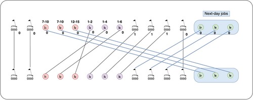
As depicted in Figure A1, the bots that executed $j_1$, $j_2$, and $j_3$ are now able to relocate as needed to perform the subsequent-day jobs $j_7$, $j_8$, and $j_9$. When relocating for next-day jobs, the return-to-station time is not a concern, as the sole constraint to be ensured in this case is the remaining distance range, which is based on battery capacity.

In a broader context, especially in scenarios involving multi-period delivery schedules, it is often the case that we only have probabilistic information regarding future jobs. To address this situation within the proposed methodological framework, and to anticipate the demand for the next day, for example, we can incorporate virtual bot jobs with late start and end times into the existing delivery schedules at the end of the day, similar to what was illustrated in Figure A1. These virtual nodes serve as probabilistic placeholders representing prospective next-day demand, which can be derived from historical data. This approach enables bots to be directed to stations with higher forecasted demand for the upcoming day at the end of the current day.

A.2. Underlying minimum cost assignment problem

In our problem, the objective is to minimise the bot fleet to feasibly execute bot jobs derived from given service schedules. This general problem is reformulated as a minimum cost assignment problem, for which we present a mathematical model in this section to make the paper self-contained.

Sets and Indices:

• $P=\{1,2,\dots ,m\}$: Set of predecessor nodes

• $Q=\{1,2,\dots ,n\}$: Set of successor nodes

Parameters:

• $c_{\mathrm{ij}}$: Cost of assigning predecessor j to successor i

Decision variables:

• $x_{\mathrm{ij}}$: Binary variable that takes the value 1 if successor j is assigned to predecessor i and 0 otherwise.

Objective function: Minimise the total cost of assignment: (A1) $\mathrm{Minimise}Z=\sum _{i\in P}\sum _{j\in Q}{c}_{\mathrm{ij}}\cdot x_{\mathrm{ij}}$(A1) Constraints: (A2) $\begin{array}{rl}& \sum _{i\in P}{x}_{\mathrm{ij}}=1\mathrm{\forall }j\in Q\end{array}$(A2) (A3) $\begin{array}{rl}& \sum _{j\in Q}{x}_{\mathrm{ij}}=1\mathrm{\forall }i\in P\end{array}$(A3) (A4) $\begin{array}{rl}& x_{\mathrm{ij}}\in \{0,1\}\mathrm{\forall }i\in P,\mathrm{\forall }j\in \mathrm{Qealigngroup}\end{array}$(A4) The objective function (A1(A1) $\mathrm{Minimise}Z=\sum _{i\in P}\sum _{j\in Q}{c}_{\mathrm{ij}}\cdot x_{\mathrm{ij}}$(A1) ) minimises the total assignment cost, while constraints (A2(A2) $\begin{array}{rl}& \sum _{i\in P}{x}_{\mathrm{ij}}=1\mathrm{\forall }j\in Q\end{array}$(A2) ) and (A3(A3) $\begin{array}{rl}& \sum _{j\in Q}{x}_{\mathrm{ij}}=1\mathrm{\forall }i\in P\end{array}$(A3) ) respectively ensure that each successor is assigned to exactly one predecessor and vice versa. The generation of nodes sets P and Q as well as assignment costs $c_{\mathrm{ij}}$ depending on the respective bot return policy are given in Section 3. Additional implementation details for each policy are provided in the following sections.

A.3. Implementation details

In every policy implementation, the construction of the assignment matrix used as input to our solution method is a critical step. It is essential to focus on defining the job2job submatrix, which determines the feasibility of executing two consecutive jobs. In the following subsection, we provide the essential pseudo-codes that define these tasks.

Assignment matrix

As an initial first step for the proposed solution framework, it is necessary to define an assignment matrix (see Figure A2), which comprises $2\cdot |J|$ rows and columns.

Figure A2. Assignment matrix structure.

The graphical illustration depicts the structure of the assignment matrix, showcasing four distinct submatrices, each with its own substructure. Specifically, these four submatrices are named: bot2bot, bot2job, job2bot, and job2job submatrix.

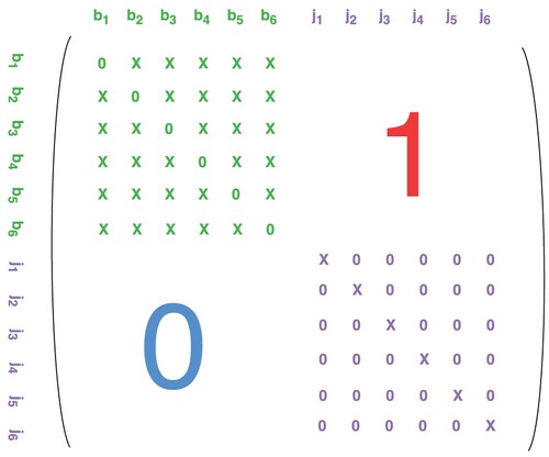
The assignment matrix is composed by the costs of each possible assignment in the bipartite graph where ‘X’ indicates an invalid assignment, with cost $w_e=\mathrm{\infty }$. This matrix displays a structure composed of four different submatrices, each of them representing one of the four possible assignment matchings: bot2bot (upper left); bot2job (upper right); job2bot (bottom left); job2job (bottom right). The bot2bot submatrix includes feasible assignments (with $w_e=0$) only alongside the main diagonal, meaning that assignments between different bots are not allowed, and when a bot is assigned to itself, it is not used to perform any job in the final solution. The bot2job submatrix only contains $w_e=1$ values since assigning a bot to a job increases the cost by one (i.e. increases the fleet size by one unit). The job2bot submatrix contains exclusively $w_e=0$ values since a job in P is assigned to a bot in Q when this is the last job executed by that bot. Finally, the job2job submatrix depends on the bot return policy to be implemented. Indeed, this submatrix indicates if two jobs can be consecutively performed by a single bot, and a cost of $w_e=0$ is associated in this case.

Dedicated-station policy

In this policy, bots return to their origin station after completing each job; hence, in order to compute which jobs are serviceable by the same bot, the following information needs to be computed: job's end time; travel time back to origin station; van routing time.

The logic behind the determination whether $j^{\mathrm{\prime }}$ and $j^{\mathrm{\prime \prime }}$ are serviceable by the same bot or not, is depicted in Algorithm 1.

In Algorithm 1, the function $\mathrm{getOriginStation}()$ takes a job as input and generates the return station for the bot performing that job as output. In this situation, we do not need a specific reference for which bot performs which job, as this will be defined in a second stage. All we need is to use the required information from the job itself: position and timing. In our notation, recall that ${\alpha }_{j^{″}}$ denotes the start time of job $j^{″}$, $f_{j^{\mathrm{\prime }}}$ the end time of job $j^{\prime }$, and $\delta (\cdot )$ is the function that computes the bot travel time between two given locations (here from the location $d_{j^{\prime }}$ of job $j^{\prime }$ to station $s_{j^{\mathrm{\prime \prime }}}$).

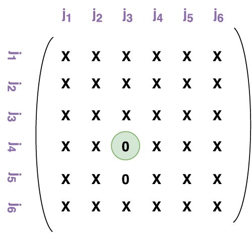
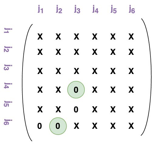
Applying Algorithm 1 to Example 1 produces the job2job submatrix as displayed in Figure A3. In this submatrix, we observe that only two pairs of jobs are serviceable by the same bot: $j_3$ and $j_4$; $j_3$ and $j_5$, and in this situation, only one of the two can be chosen in the final matching.

Figure A3. job2job submatrix for Example 1 under the dedicated-station policy.

The illustration depicts the job2job submatrix for Example 1, representing the costs of consecutively performing one job after another using the same bot. A cost of zero is assigned only when two jobs can be executed consecutively by the same bot. Specifically, the displayed job2job submatrix corresponds to Example 1 under the dedicated-station policy, where the optimal solution involves selecting only one element with a cost of zero from the submatrix.

Closest-station policy

Under the closest-station policy, it may occur that a bot is picked up from one bot station to service a specific customer but returns to another station which is closer to the performed job's location.

In this case, the precomputation of the job2job submatrix follows the logic depicted in Algorithm 2.

In Algorithm 2, the function $\mathrm{getClosestStation}()$ takes a job as input and generates the closest station relative to the position of the input job as output. As for the dedicated-station policy, all the needed information is taken from the job itself: position and timing.

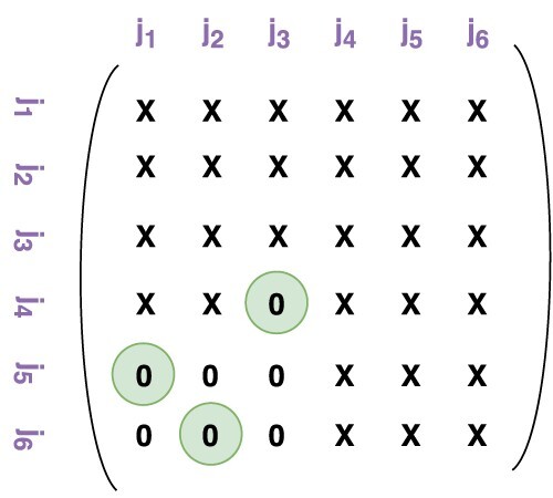
Applying Algorithm 2 to Example 1 produces the job2job submatrix as displayed in Figure A4, where the costs ($w_e=0$) of the chosen edges in the optimal matching have been highlighted in green.

Figure A4. job2job submatrix for Example 1 under the closest-station policy.

The illustration depicts the job2job submatrix for Example 1, representing costs for consecutively performing one job after another using the same bot. A cost of zero is assigned only when two jobs can be executed consecutively by the same bot. Specifically, the displayed job2job submatrix corresponds to Example 1 under the closest-station policy, where the optimal solution involves selecting two elements with a cost of zero from the submatrix.

Most-suitable station policy

The most-suitable-station policy offers bots with even more flexibility to switch between bot stations. Algorithm 3 provides with the pseudocode for the conditions that allow two jobs to be performed consecutively in this situation, and therefore obtain the associated job2job submatrix.

In Algorithm A5, the function $\mathrm{returnToStationT}(j,s_i)$ generates the arrival time for a bot moving from job j to station $s_i$. The function $\mathrm{vanArrivalTAtStation}(v,s_i)$ takes a van v and a station $s_i$ as input and provides the time at which v visits $s_i$ during its route as output.

Figure A5. job2job submatrix for Example 1 under the most-suitable-station policy.

The illustration shows, for Example 1, the job2job submatrix indicating the costs of performing one job after another using the same bot. The cost is set to zero only when two jobs can be performed by the same bot consecutively. More precisely, the submatrix illustrates the job2job submatrix for Example 1 under the most-suitable-station policy where three elements of the submatrix with a cost of zero are selected in the optimal solution.

Applying Algorithm 3 to Example 1 produces the job2job submatrix as displayed in Figure A5, where, as before, the costs ($w_e=0$) of the chosen edges in the optimal matching have been highlighted in green.

Closest-station policy and most-suitable-station policy with relocation nodes

As depicted in Figure A6, the introduction of relocation nodes extends the assignment matrix previously defined as new edges may now appear. More precisely, the assignment matrix has to store the costs relative to the possible connections between the relocation nodes and with the other types of nodes. In Figure A6, due to space limitations, relocation is abbreviated as rel except for the relocation2relocation submatrix which is labelled r2r.

Figure A6. Extended assignment matrix structure with relocation nodes.

The figure represents a graphical illustration showing the extended structure of the assignment matrix when relocation nodes are added to the structure.

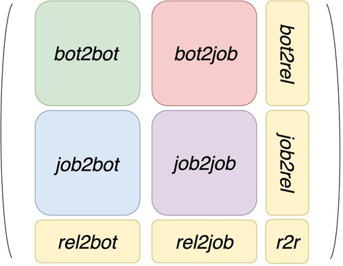
The extended assignment matrix remains a square matrix but its dimension is increased by the number of available relocation nodes. The new submatrix costs need to be computed following the rules of each new edge typology added to the solution framework. The bot2relocation and relocation2bot submatrices are easily constructed, as no assignment is allowed between relocation nodes and bot nodes (i.e. only invalid assignments with cost $w_e=\mathrm{\infty }$). relocation2relocation edges have a cost $w_e=0$ only when the relocation node is not used; in all the other cases the assignment is not allowed and $w_e=\mathrm{\infty }$.

The steps followed to decide on the feasible assignments in the relocation2job and job2relocation submatrices are depicted in Algorithm 4.

In Example 2, no job can be performed by a bot transported by the black van using a relocation node. On the contrary, the blue van could transport one bot from $s_1$ to $s_2$, using the $r_{s_1{s}_2}$ relocation node, and $j_3$ could be performed by this same bot. Therefore, in submatrix job2rel, the entry $j_3$-$r_{s_1{s}_2}$ is given a cost $w_e=0$. Following the same logic, $r_{s_1{s}_2}$-$j_3$ in the rel2job submatrix is given a cost $w_e=0$.

References

- Agatz, N., P. Bouman, and M. Schmidt. 2018. “Optimization Approaches for the Traveling Salesman Problem with Drone.” Transportation Science 52 (4): 965–981. https://doi.org/10.1287/trsc.2017.0791.
- Alfandari, L., I. Ljubić, and M. D. M. da Silva. 2022. “A Tailored Benders Decomposition Approach for Last-mile Delivery with Autonomous Robots.” European Journal of Operational Research 299 (2): 510–525. https://doi.org/10.1016/j.ejor.2021.06.048.
- Bakach, I., A. M. Campbell, and J. F. Ehmke. 2021. “A Two-tier Urban Delivery Network with Robot-based Deliveries.” Networks 78 (4): 461–483. https://doi.org/10.1002/net.v78.4.
- Bertossi, A. A., P. Carraresi, and G. Gallo. 1987. “On Some Matching Problems Arising in Vehicle Scheduling Models.” Networks 17 (3): 271–281. https://doi.org/10.1002/net.v17:3.
- Boysen, N., D. Briskorn, S. Fedtke, and S. Schwerdfeger. 2018. “Drone Delivery From Trucks: Drone Scheduling for Given Truck Routes.” Networks 72 (4): 506–527. https://doi.org/10.1002/net.v72.4.
- Boysen, N., and S. Emde. 2014. “Scheduling the Part Supply of Mixed-model Assembly Lines in Line-integrated Supermarkets.” European Journal of Operational Research 239 (3): 820–829. https://doi.org/10.1016/j.ejor.2014.05.029.
- Boysen, N., S. Fedtke, and S. Schwerdfeger. 2021. “Last-mile Delivery Concepts: a Survey From An Operational Research Perspective.” OR Spectrum 43 (1): 1–58. https://doi.org/10.1007/s00291-020-00607-8.
- Boysen, N., S. Schwerdfeger, and F. Weidinger. 2018. “Scheduling Last-mile Deliveries with Truck-based Autonomous Robots.” European Journal of Operational Research 271 (3): 1085–1099. https://doi.org/10.1016/j.ejor.2018.05.058.
- Chen, C., E. Demir, and Y. Huang. 2021. “An Adaptive Large Neighborhood Search Heuristic for the Vehicle Routing Problem with Time Windows and Delivery Robots.” European Journal of Operational Research 294 (3): 1164–1180. https://doi.org/10.1016/j.ejor.2021.02.027.
- Chen, C., E. Demir, Y. Huang, and R. Qiu. 2021. “The Adoption of Self-driving Delivery Robots in Last Mile Logistics.” Transportation Research Part E: Logistics and Transportation Review 146:102214. https://doi.org/10.1016/j.tre.2020.102214.
- Freitas, J. C., P. H. V. Penna, and T. A. Toffolo. 2023. “Exact and Heuristic Approaches to Truck–drone Delivery Problems.” EURO Journal on Transportation and Logistics 12:100094. https://doi.org/10.1016/j.ejtl.2022.100094.
- Heimfarth, A., M. Ostermeier, and A. Hübner. 2022. “A Mixed Truck and Robot Delivery Approach for the Daily Supply of Customers.” European Journal of Operational Research 303 (1): 401–421. https://doi.org/10.1016/j.ejor.2022.02.028.
- Hu, W., J. Dong, B.-G. Hwang, R. Ren, and Z. Chen. 2019. “A Scientometrics Review on City Logistics Literature: Research Trends, Advanced Theory and Practice.” Sustainability 11 (10): 2724. https://doi.org/10.3390/su11102724.
- Joerss, M., J. Schroder, F. Neuhaus, C. Klink, and F. Mann. 2016. “Parcel Delivery: The Future of Last Mile.” McKinsey & Company Report.
- Jun, S., C. H. Choi, and S. Lee. 2022. “Scheduling of Autonomous Mobile Robots with Conflict-free Routes Utilising Contextual-bandit-based Local Search.” International Journal of Production Research60 (13): 4090–4116. https://doi.org/10.1080/00207543.2022.2063085.
- Kim, S., and I. Moon. 2018. “Traveling Salesman Problem with a Drone Station.” IEEE Transactions on Systems, Man, and Cybernetics: Systems 49 (1): 42–52. https://doi.org/10.1109/TSMC.2018.2867496.
- Kuhn, H. W.. 1955. “The Hungarian Method for the Assignment Problem.” Naval Research Logistics Quarterly 2 (1-2): 83–97. https://doi.org/10.1002/nav.v2:1/2.
- Li, F., and O. Kunze. 2023. “A Comparative Review of Air Drones (UAVs) and Delivery Bots (SUGVs) for Automated Last Mile Home Delivery.” Logistics 7 (2): 21. https://doi.org/10.3390/logistics7020021.
- Lim, S. F. W., X. Jin, and J. S. Srai. 2018. “Consumer-driven E-commerce: A Literature Review, Design Framework, and Research Agenda on Last-mile Logistics Models.” International Journal of Physical Distribution & Logistics Management 48 (3): 308–332. https://doi.org/10.1108/IJPDLM-02-2017-0081.
- Liu, D., E. I. Kaisar, Y. Yang, and P. Yan. 2022. “Physical Internet-enabled E-grocery Delivery Network: A Load-dependent Two-echelon Vehicle Routing Problem with Mixed Vehicles.” International Journal of Production Economics 254:108632. https://doi.org/10.1016/j.ijpe.2022.108632.
- Mourad, A., J. Puchinger, and T. V. Woensel. 2021. “Integrating Autonomous Delivery Service Into a Passenger Transportation System.” International Journal of Production Research 59 (7): 2116–2139. https://doi.org/10.1080/00207543.2020.1746850.
- Murray, C. C., and A. G. Chu. 2015. “The Flying Sidekick Traveling Salesman Problem: Optimization of Drone-assisted Parcel Delivery.” Transportation Research Part C: Emerging Technologies 54:86–109. https://doi.org/10.1016/j.trc.2015.03.005.
- Ostermeier, M., A. Heimfarth, and A. Hübner. 2022. “Cost-optimal Truck-and-robot Routing for Last-mile Delivery.” Networks 79 (3): 364–389. https://doi.org/10.1002/net.v79.3.
- Ostermeier, M., A. Heimfarth, and A. Hübner. 2023. “The Multi-vehicle Truck-and-robot Routing Problem for Last-mile Delivery.” European Journal of Operational Research 310 (2): 680–697. https://doi.org/10.1016/j.ejor.2023.03.031.
- Otto, A., and O. Battaïa. 2017. “Reducing Physical Ergonomic Risks At Assembly Lines by Line Balancing and Job Rotation: A Survey.” Computers & Industrial Engineering 111:467–480. https://doi.org/10.1016/j.cie.2017.04.011.
- Peterson, H. 2018. Missing Wages, Grueling Shifts, and Bottles of Urine: The Disturbing Accounts of Amazon Delivery Drivers May Reveal the True Human Cost of 'free' Shipping.” Business Insider.
- Pugliese, L. D. P., G. Macrina, and F. Guerriero. 2021. “Trucks and Drones Cooperation in the Last-mile Delivery Process.” Networks 78 (4): 371–399. https://doi.org/10.1002/net.v78.4.
- Simoni, M. D., E. Kutanoglu, and C. G. Claudel. 2020. “Optimization and Analysis of a Robot-assisted Last Mile Delivery System.” Transportation Research Part E: Logistics and Transportation Review142:102049. https://doi.org/10.1016/j.tre.2020.102049.
- Srinivas, S., S. Ramachandiran, and S. Rajendran. 2022. “Autonomous Robot-driven Deliveries: A Review of Recent Developments and Future Directions.” Transportation Research Part E: Logistics and Transportation Review 165:102834. https://doi.org/10.1016/j.tre.2022.102834.
- Voccia, S. A., A. M. Campbell, and B. W. Thomas. 2019. “The Same-day Delivery Problem for Online Purchases.” Transportation Science 53 (1): 167–184. https://doi.org/10.1287/trsc.2016.0732.
- Yang, Y., C. Yan, Y. Cao, and R. Roberti. 2023. “Planning Robust Drone-truck Delivery Routes Under Road Traffic Uncertainty.” European Journal of Operational Research 309 (3): 1145–1160. https://doi.org/10.1016/j.ejor.2023.02.031.
- Yu, S., J. Puchinger, and S. Sun. 2023. “Electric Van-based Robot Deliveries with En-route Charging.” European Journal of Operational Research.
- Zou, B., S. Wu, Y. Gong, Z. Yuan, and Y. Shi. 2023. “Delivery Network Design of a Locker-drone Delivery System.” International Journal of Production Research: 1–25. https://doi.org/10.1080/00207543.2023.2254402.