High-order fully actuated system approaches: Part II. Generalized strict-feedback systems

Abstract

An advantage of a high-order fully-actuated (HOFA) system is that there exists a controller such that a constant linear closed-loop system with an arbitrarily assignable eigenstructure can be obtained. In this paper, a generalised form of the conventional first-order strict-feedback systems (SFSs) is firstly proposed, and a recursive solution is proposed to convert equivalently the generalised SFS into a HOFA model. Then the second- and high-order SFSs are defined and their equivalent HOFA models are also derived. It is further shown that, under certain common conditions, the recursive solutions for converting the generalised SFSs into HOFA models can be rearranged into direct analytical explicit solutions. Such a high-order system approach is more direct and simpler than the first-order system approach since it avoids the process of converting firstly these second- and high-order SFSs into first-order ones for control, and can finally produce a constant linear closed-loop system. Particularly, it is more effective than the well-known method of backstepping since, for the generalised complicated SFSs with more subsystems, the method of backstepping may simply be not applicable due to more serious ‘differential explosion’ problem. Two examples are worked out to demonstrate the effect of the approach.

Keywords:

• Strict-feedback systems
• high-order systems
• full-actuation
• recursive solutions
• explicit solutions

1. Introduction

State-space approaches for control system analysis and design have remained absolutely dominant for over a half century, yet it is found that state-space models may not be the best choice for dealing with the control of the system, although they are probably the best choice for state solutions (response analysis) and observations (estimations) (see, Duan, 2020a, 2020b, 2020c, 2020d). In contrast, a type of high-order fully-actuated (HOFA) system models behave more powerfully in the control of many nonlinear systems (Duan, 2020a, 2020d). This paper is concerned with the derivation of the HOFA models of three types of generalised strict-feedback nonlinear systems.

1.1. Typical SFSs

Consider the following strict-feedback nonlinear system (1) $\left\{\begin{array}{l}{\dot{x}}_1=f_1\left(x_1\right)+G_1\left(x_1\right)x_2\\ {\dot{x}}_2=f_2(x_1,x_2)+G_2(x_1,x_2)x_3\\ ⋮\\ {\dot{x}}_{n-1}=f_{n-1}(x_1,\dots ,x_{n-1})+G_{n-1}(x_1,\dots ,x_{n-1})x_n\\ {\dot{x}}_n=f_n(x_1,\dots ,x_n)+G_n(x_1,\dots ,x_n)u,\end{array}\right.$(1) where $x_i\in {\mathbb{R}}^r$, $i=1,2,\dots ,n$ are the state vectors, $u\in {\mathbb{R}}^r$ is the control input, $f_i(x_1,\dots ,x_i)\in {\mathbb{R}}^r$ and $G_i(x_1,\dots ,x_i)\in {\mathbb{R}}^{r\times r}$, $i=1,2,\dots ,n$ are sufficiently smooth vector functions and matrix functions, respectively. Furthermore, $G_i(x_1,\dots ,x_i)$ is nonsingular for all $x_i\in {\mathbb{R}}^r$, $i=1,2,\dots ,n.$

This type of systems are called in the literature the strict-feedback systems (SFSs), which are extremely important due to the following three aspects.

Firstly, more general nonlinear systems can be equivalently converted into the form. In fact, it has been shown that the general nonlinear systems in the following affine form $\dot{x}=f\left(x\right)+g\left(x\right)u,$ with $x\in {\mathbb{R}}^n$ and $u\in {\mathbb{R}}^r$ being respectively the state and control vectors, can be converted into the form of (10(10) $\left\{\begin{array}{l}u=-L_n^{-1}\left(A_{0\sim n-1}{z^{(0\sim n-1)}+u}^{\ast }\right)\\ u^{\ast }=h_n(z^{(0\sim n-1)},\zeta ,t)-v,\end{array}\right.$(10) ) under some conditions (Kanellakopoulos et al., 1991; Krstic et al., 1995; Riccardo & Tomei, 1995). Very recently, Duan (2020d) investigated a more general system in the form of $x^{\left(m\right)}=f(x,\dot{x},\dots ,x^{(m-1)})+G(x,\dot{x},\dots ,x^{(m-1)})u,$ where $m\ge 1$ is some integer, $x\in {\mathbb{R}}^n$ and $u\in {\mathbb{R}}^r$ are respectively the state and control vectors. It is shown that the system, when n is a multiple of r, can also be converted, under certain conditions, into a similar strict-feedback form of order m (Duan, 2020d), which reduces to the normal SFS form of (10(10) $\left\{\begin{array}{l}u=-L_n^{-1}\left(A_{0\sim n-1}{z^{(0\sim n-1)}+u}^{\ast }\right)\\ u^{\ast }=h_n(z^{(0\sim n-1)},\zeta ,t)-v,\end{array}\right.$(10) ) in the case of m = 1. Such facts indicate, from the theoretical aspect, that SFSs are a type of very common nonlinear systems.

Secondly, SFSs describe a variety of practical nonlinear systems. Such a fact has been verified by a great deal of applications, including, but certainly not limited to, circuit system (Khalil, 2002), pendulum systems (Jiang & Nijmeijer, 1997; Khalil, 2002; Yang et al., 2004), robotic systems (Dawson et al., 1994; Ferrara & Giacomini, 2000; Jiang & Nijmeijer, 1997; Khalil, 2002; Riccardo & Tomei, 1995; Yang et al., 2004), missile and satellite control systems (Farrell et al., 2005; Kim et al., 2004; Sun et al., 2017), and ship fin roll stabilisation systems (Yang et al., 2004).

Thirdly, SFSs probably form the largest class of nonlinear systems for which stabilising controllers can be systematically designed. A very typical recursive design method for this class of systems is the well-known method of backstepping, which were initiated by a group of researchers, e.g. Tsinias (1989, 1991), Byrnes and Isidori (1989), Sontag and Sussmann (1988), Kokotovic and Sussmann (1989), and Saberi et al. (1990). Since 1990, works on control of SFSs using improved method of backstepping have dramatically increased (Farrell et al., 2009; Hong & Jiang, 2006; Huang et al., 2005; Kokotovic & Arcak, 2001; Tee & Ge, 2011).

1.2. HOFA system approaches

Very recently, it is pointed out, and also fully evidenced, in Duan (2020a, 2020b, 2020d) that the commonly used first-order state-space models are, although very convenient for problems of state solutions and observations, not effective enough for nonlinear system control, while the type of HOFA system models, proposed in Duan (2020a, 2020d), are more effective and convenient for control design of nonlinear systems. It is shown in Duan (2020a, 2020d) that, once a HOFA model for a nonlinear system is obtained, the controller can then be immediately written out, which eliminates the nonlinearities in the system, and eventually results in a constant linear closed-loop system.

The HOFA system approaches actually solve many problems that the first-order Lyapunov stabilisation approach does not solve. In fact, the first-order state-space stabilisation approach based on Lyapunov functions analysis depends heavily on the complexity of the nonlinearities. Therefore, it may not even provide a solution in certain complex cases, to say nothing of giving some global stability results or producing constant linear closed-loop systems. While the HOFA system approaches make use of the full-actuation feature and can eliminate easily the nonlinearities, no matter how complicated they are, theoretically.

Clearly, in the applications of the HOFA system approaches for control systems design, the main task is to derive a HOFA model for the considered system. In Duan (2020a), a simplified version of the SFS is proven to be equivalent to a HOFA system. In this paper, the SFS (10(10) $\left\{\begin{array}{l}u=-L_n^{-1}\left(A_{0\sim n-1}{z^{(0\sim n-1)}+u}^{\ast }\right)\\ u^{\ast }=h_n(z^{(0\sim n-1)},\zeta ,t)-v,\end{array}\right.$(10) ) is firstly generalised into a more complicated form, and then it is shown that a recursive solution exists to convert the generalised SFS equivalently into a HOFA model.

Most practical systems are governed by physical laws, such as, Newton's law, Lagrangian equation, Theorem of linear and angular momentum, Kirchhoff's laws of current and voltage, etc. When modelled by these physical laws, a set of subsystems of second- or higher-order are firstly obtained (Duan, 2020e, 2020f; Spong et al., 2008). In view of such a fact, generalised SFSs of both second-order and high-order are also proposed in this paper. Similarly to the generalised first-order case, recursive solutions to convert the generalised second-order and high-order SFSs equivalently into some HOFA models are also proposed. Therefore, control of these systems can then be easily realised and better solved in the sense that the final closed-loop system is a constant and linear one with a desired eigenstructure. While on the other side, due to the complexity in the generalised SFSs, the typical method of backstepping may not be applicable especially when n is large due to possible more serious ‘differential explosion’ phenomenon.

In this paper, we use $C(k,n)$ to denote the combination of k elements out of n. Furthermore, for $x,x_i\in {\mathbb{R}}^m,$ and $A_i\in {\mathbb{R}}^{m\times m},$ $n_0,n_i\in \mathbb{N},n_0<n_i,$ $i=1,2,\dots ,n,$ the following symbols are frequently used in the paper: $\begin{array}{rl}{x}^{(0\sim n)}& =\left[\begin{array}{c}x\\ \dot{x}\\ ⋮\\ x^{\left(n\right)}\end{array}\right],\\ x_{i\sim j}^{(0\sim n)}& =\left[\begin{array}{c}{x}_i^{(0\sim n)}\\ x_{i+1}^{(0\sim n)}\\ ⋮\\ x_j^{(0\sim n)}\end{array}\right],j\ge i,\\ x_k^{(n_0\sim n_k)}{|}_{k=i\sim j}& =\left[\begin{array}{c}{x}_i^{(n_0\sim n_i)}\\ x_{i+1}^{(n_0\sim n_{i+1})}\\ ⋮\\ x_j^{(n_0\sim n_j)}\end{array}\right],j\ge i,\\ A_{0\sim n}& =\left[A_0{A}_1\cdots A_n\right],\\ \mathrm{\Phi }\left(A_{0\sim n}\right)& =\left[\begin{array}{cccc}0& I& & \\ & & \ddots & \\ & & & I\\ -A_0& -A_1& \cdots & -A_n\end{array}\right].\end{array}$

2. Generalized SFSs

2.1. First-order SFSs

The SFS (10(10) $\left\{\begin{array}{l}u=-L_n^{-1}\left(A_{0\sim n-1}{z^{(0\sim n-1)}+u}^{\ast }\right)\\ u^{\ast }=h_n(z^{(0\sim n-1)},\zeta ,t)-v,\end{array}\right.$(10) ) is a normal one, and can be further generalised.

Consider a system in the following first-order descriptor form (Duan, 2010) (2) $E(x,t)\dot{x}=f(x,t),$(2) where $x\in {\mathbb{R}}^r$ is the state vector, $f(\cdot ,\cdot )\in {\mathbb{R}}^r$ is a continuous vector function, $E(x,t)\in {\mathbb{R}}^{r\times r}$ can be singular. When the matrix $E(x,t)$ is not diagonal, once (2(2) $E(x,t)\dot{x}=f(x,t),$(2) ) is expanded, the ith equation may contain the derivative of the jth state variable. In such a case, the derivative of the jth state variable in the ith equation can also be shifted into the function $f(x,t)$.

We use this idea to generalise the above strict-feedback nonlinear system (10(10) $\left\{\begin{array}{l}u=-L_n^{-1}\left(A_{0\sim n-1}{z^{(0\sim n-1)}+u}^{\ast }\right)\\ u^{\ast }=h_n(z^{(0\sim n-1)},\zeta ,t)-v,\end{array}\right.$(10) ). Specifically, we add the derivative term of the state components, the time variable t and a parameter vector $\zeta \in {\mathbb{R}}^m$ to each pair of f and G functions, so as to obtain the following generalised form: (3) $\left\{\begin{array}{l}{\dot{x}}_1=f_1(x_1,\zeta ,t)+G_1(x_1,\zeta ,t)x_2\\ {\dot{x}}_2=f_2(x_1^{(0\sim 1)},x_2,\zeta ,t)+G_2(x_1^{(0\sim 1)},x_2,\zeta ,t)x_3\\ ⋮\\ {\dot{x}}_{n-1}=f_{n-1}(x_{1\sim n-2}^{(0\sim 1)},x_{n-1},\zeta ,t)\\ +G_{n-1}(x_{1\sim n-2}^{(0\sim 1)},x_{n-1},\zeta ,t)x_n\\ {\dot{x}}_n=f_n(x_{1\sim n-1}^{(0\sim 1)},x_n,\zeta ,t)+G_n(x_{1\sim n-1}^{(0\sim 1)},x_n,\zeta ,t)u.\end{array}\right.$(3) where $x_i\in {\mathbb{R}}^r$, $i=1,2,\dots ,n$ are the state vectors, $u\in {\mathbb{R}}^r$ is the control input, $f_i(x_{1\sim i-1}^{(0\sim 1)},x_i,\zeta ,t)\in {\mathbb{R}}^r$ and $G_i(x_{1\sim i-1}^{(0\sim 1)},x_i,\zeta ,t)\in {\mathbb{R}}^{r\times r}$, $i=1,2,\dots ,n$ are sufficiently smooth vector functions and matrix functions, respectively.

As a normal requirement to SFSs, we assume the following:

Assumption A1

For arbitrary $x_i\in {\mathbb{R}}^r,i=1,2,\dots ,n$, and $\zeta \in {\mathbb{R}}^m$, there holds (4) $det{G}_i(x_{1\sim i-1}^{(0\sim 1)},x_i,\zeta ,t)\ne 0,\mathrm{\forall }t\ge 0.$(4)

In certain high-dimensional cases, the above Assumption A1 may be difficult to verify. It is recommanded that symbolic computation techniques may be considered to help in such cases.

For this generalised form (3(3) $\left\{\begin{array}{l}{\dot{x}}_1=f_1(x_1,\zeta ,t)+G_1(x_1,\zeta ,t)x_2\\ {\dot{x}}_2=f_2(x_1^{(0\sim 1)},x_2,\zeta ,t)+G_2(x_1^{(0\sim 1)},x_2,\zeta ,t)x_3\\ ⋮\\ {\dot{x}}_{n-1}=f_{n-1}(x_{1\sim n-2}^{(0\sim 1)},x_{n-1},\zeta ,t)\\ +G_{n-1}(x_{1\sim n-2}^{(0\sim 1)},x_{n-1},\zeta ,t)x_n\\ {\dot{x}}_n=f_n(x_{1\sim n-1}^{(0\sim 1)},x_n,\zeta ,t)+G_n(x_{1\sim n-1}^{(0\sim 1)},x_n,\zeta ,t)u.\end{array}\right.$(3) ), some existing control methods, such as the backstepping methods, may become extremely difficult or even impossible to apply when r and n are large due to the ‘differential explosion’ problem. However, if we can transform it into a HOFA system model, its control problems can then be solved easily and conveniently (Duan, 2020a).

Theorem 2.1

Let Assumption A1 be satisfied, then, under the following transformation (5) $\left\{\begin{array}{l}{x}_1=z\\ x_2=G_1^{-1}(z,\zeta ,t)[\dot{z}-f_1(z,\zeta ,t\left)\right]\\ x_{k+1}=L_k^{-1}(z^{(0\sim k-1)},\zeta ,t)[z^{\left(k\right)}-h_k(z^{(0\sim k-1)},\zeta ,t\left)\right]\\ k=2,3,\dots ,n-1,\end{array}\right.$(5) the generalised strict-feedback nonlinear system (3(3) $\left\{\begin{array}{l}{\dot{x}}_1=f_1(x_1,\zeta ,t)+G_1(x_1,\zeta ,t)x_2\\ {\dot{x}}_2=f_2(x_1^{(0\sim 1)},x_2,\zeta ,t)+G_2(x_1^{(0\sim 1)},x_2,\zeta ,t)x_3\\ ⋮\\ {\dot{x}}_{n-1}=f_{n-1}(x_{1\sim n-2}^{(0\sim 1)},x_{n-1},\zeta ,t)\\ +G_{n-1}(x_{1\sim n-2}^{(0\sim 1)},x_{n-1},\zeta ,t)x_n\\ {\dot{x}}_n=f_n(x_{1\sim n-1}^{(0\sim 1)},x_n,\zeta ,t)+G_n(x_{1\sim n-1}^{(0\sim 1)},x_n,\zeta ,t)u.\end{array}\right.$(3) ) can be transformed into the following HOFA system (6) $z^{\left(n\right)}=h_n(z^{(0\sim n-1)},\zeta ,t)+L_n(z^{(0\sim n-1)},\zeta ,t)u,$(6) where the matrix function $L_k(z^{(0\sim k-1)},\zeta ,t)$ and the vector function $h_k(z^{(0\sim k-1)},\zeta ,t)$ are recursively given by (7) $\begin{array}{rl}& L_k(z^{(0\sim k-1)},\zeta ,t)\\ & =L_{k-1}(z^{(0\sim k-2)},\zeta ,t)G_k(x_{1\sim k-1}^{(0\sim 1)},x_k,\zeta ,t),\end{array}$(7) and (8) $\begin{array}{rl}& h_k(z^{(0\sim k-1)},\zeta ,t)\\ & ={\dot{h}}_{k-1}(z^{(0\sim k-2)},\zeta ,t)+{\dot{L}}_{k-1}(z^{(0\sim k-2)},\zeta ,t)x_k\\ & +L_{k-1}(z^{(0\sim k-2)},\zeta ,t)f_k(x_{1\sim k-1}^{(0\sim 1)},x_k,\zeta ,t),\\ & k=1,2,\dots ,n\end{array}$(8) with the initial values (9) $L_0(\zeta ,t)=I_r,h_0(\zeta ,t)=0,$(9) where in (7(7) $\begin{array}{rl}& L_k(z^{(0\sim k-1)},\zeta ,t)\\ & =L_{k-1}(z^{(0\sim k-2)},\zeta ,t)G_k(x_{1\sim k-1}^{(0\sim 1)},x_k,\zeta ,t),\end{array}$(7) )–(8(8) $\begin{array}{rl}& h_k(z^{(0\sim k-1)},\zeta ,t)\\ & ={\dot{h}}_{k-1}(z^{(0\sim k-2)},\zeta ,t)+{\dot{L}}_{k-1}(z^{(0\sim k-2)},\zeta ,t)x_k\\ & +L_{k-1}(z^{(0\sim k-2)},\zeta ,t)f_k(x_{1\sim k-1}^{(0\sim 1)},x_k,\zeta ,t),\\ & k=1,2,\dots ,n\end{array}$(8) ) the $x_i,i=2,3,\dots ,n$ and their derivatives are all given or determined by the transformation (5(5) $\left\{\begin{array}{l}{x}_1=z\\ x_2=G_1^{-1}(z,\zeta ,t)[\dot{z}-f_1(z,\zeta ,t\left)\right]\\ x_{k+1}=L_k^{-1}(z^{(0\sim k-1)},\zeta ,t)[z^{\left(k\right)}-h_k(z^{(0\sim k-1)},\zeta ,t\left)\right]\\ k=2,3,\dots ,n-1,\end{array}\right.$(5) ).

For a proof of the theorem, please refer to the Appendix.

Remark 2.1

The Assumption A1 is a global one, it requires (4(4) $det{G}_i(x_{1\sim i-1}^{(0\sim 1)},x_i,\zeta ,t)\ne 0,\mathrm{\forall }t\ge 0.$(4) ) to hold for $x_i\in {\mathbb{R}}^r,i=1,2,\dots ,n$. Relaxation of this assumption to a local one can be considered. If this assumption is valid only on a certain set $\mathrm{\Omega }\subset {\mathbb{R}}^{nr}$, then the derived high-order system (6(6) $z^{\left(n\right)}=h_n(z^{(0\sim n-1)},\zeta ,t)+L_n(z^{(0\sim n-1)},\zeta ,t)u,$(6) ) is a HOFA model on a certain set ${\mathrm{\Omega }}^{\mathrm{\prime }}$ determined from Ω by the transformation (5(5) $\left\{\begin{array}{l}{x}_1=z\\ x_2=G_1^{-1}(z,\zeta ,t)[\dot{z}-f_1(z,\zeta ,t\left)\right]\\ x_{k+1}=L_k^{-1}(z^{(0\sim k-1)},\zeta ,t)[z^{\left(k\right)}-h_k(z^{(0\sim k-1)},\zeta ,t\left)\right]\\ k=2,3,\dots ,n-1,\end{array}\right.$(5) ).

Remark 2.2

Once the HOFA model (6(6) $z^{\left(n\right)}=h_n(z^{(0\sim n-1)},\zeta ,t)+L_n(z^{(0\sim n-1)},\zeta ,t)u,$(6) ) is obtained, the controller of the system can then be simply designed as (Duan, 2020a, 2020d) (10) $\left\{\begin{array}{l}u=-L_n^{-1}\left(A_{0\sim n-1}{z^{(0\sim n-1)}+u}^{\ast }\right)\\ u^{\ast }=h_n(z^{(0\sim n-1)},\zeta ,t)-v,\end{array}\right.$(10) which gives the following constant linear closed-loop system $z^{\left(n\right)}+A_{0\sim n-1}{z}^{(0\sim n-1)}=v,$ where v is some external signal, while $A_{0\sim n-1}$ is an arbitrary matrix which makes $\mathrm{\Phi }\left(A_{0\sim n-1}\right)$ stable. A complete parametric approach for solving the matrix $A_{0\sim n-1}$ is given in Duan (2020a) (see also the Proposition 2 in Duan, 2020d).

2.2. Second-order SFSs

Lagrangian Equation and Theorem of Momentum (moment) are often used in modelling physical systems. As a result in such applications, the models of the obtained subsystems are of second-order. For this reason, we introduce the following second-order strict-feedback nonlinear system: (11) $\left\{\begin{array}{l}{\ddot{x}}_1=f_1(x_1,{\dot{x}}_1,\zeta ,t)+G_1(x_1,{\dot{x}}_1,\zeta ,t)x_2\\ {\ddot{x}}_2=f_2(x_1^{(0\sim 2)},x_2^{(0\sim 1)},\zeta ,t)\\ +G_2(x_1^{(0\sim 2)},x_2^{(0\sim 1)},\zeta ,t)x_3\\ ⋮\\ {\ddot{x}}_{n-1}=f_{n-1}(x_{1\sim n-2}^{(0\sim 2)},x_{n-1}^{(0\sim 1)},\zeta ,t)\\ +G_{n-1}(x_{1\sim n-2}^{(0\sim 2)},x_{n-1}^{(0\sim 1)},\zeta ,t)x_n\\ {\ddot{x}}_n=f_n(x_{1\sim n-1}^{(0\sim 2)},x_n^{(0\sim 1)},\zeta ,t)\\ +G_n(x_{1\sim n-1}^{(0\sim 2)},x_n^{(0\sim 1)},\zeta ,t)u,\end{array}\right.$(11) where $x_i\in {\mathbb{R}}^r$, $i=1,2,\dots ,n$ are the state vectors, $u\in {\mathbb{R}}^r$ is the control input vector, $\zeta \in {\mathbb{R}}^m$ is a parameter vector; $f_i(x_{1\sim i-1}^{(0\sim 2)},x_i^{(0\sim 1)},\zeta ,t)\in {\mathbb{R}}^r$, $i=1,2,\dots ,n$ are a set of sufficiently smooth vector functions, $G_i(x_{1\sim i-1}^{(0\sim 2)},x_i^{(0\sim 1)},\zeta ,t)\in {\mathbb{R}}^{r\times r}$, $i=1,2,\dots ,n$ are a set of sufficiently smooth matrix functions, and satisfy the following assumption:

Assumption A2

For arbitrary $x_i\in {\mathbb{R}}^r,i=1,2,\dots ,n$, and $\zeta \in {\mathbb{R}}^m$, there holds $det{G}_i(x_{1\sim i-1}^{(0\sim 2)},x_i^{(0\sim 1)},\zeta ,t)\ne 0,\mathrm{\forall }t\ge 0.$

Parallel to the first-order case, we have the following conclusion.

Theorem 2.2

Let Assumption A2 be met, then, under the following transformation (12) $\left\{\begin{array}{l}{x}_1=z\\ x_2=G_1^{-1}(z^{(0\sim 1)},\zeta ,t)[\ddot{z}-f_1(z^{(0\sim 1)},\zeta ,t\left)\right]\\ x_{k+1}=L_k^{-1}(z^{(0\sim 2k-1)},\zeta ,t)\\ \times [z^{\left(2k\right)}-h_k(z^{(0\sim 2k-1)},\zeta ,t\left)\right],\\ k=2,3,\dots ,n-1\end{array}\right.$(12) the SFS (11(11) $\left\{\begin{array}{l}{\ddot{x}}_1=f_1(x_1,{\dot{x}}_1,\zeta ,t)+G_1(x_1,{\dot{x}}_1,\zeta ,t)x_2\\ {\ddot{x}}_2=f_2(x_1^{(0\sim 2)},x_2^{(0\sim 1)},\zeta ,t)\\ +G_2(x_1^{(0\sim 2)},x_2^{(0\sim 1)},\zeta ,t)x_3\\ ⋮\\ {\ddot{x}}_{n-1}=f_{n-1}(x_{1\sim n-2}^{(0\sim 2)},x_{n-1}^{(0\sim 1)},\zeta ,t)\\ +G_{n-1}(x_{1\sim n-2}^{(0\sim 2)},x_{n-1}^{(0\sim 1)},\zeta ,t)x_n\\ {\ddot{x}}_n=f_n(x_{1\sim n-1}^{(0\sim 2)},x_n^{(0\sim 1)},\zeta ,t)\\ +G_n(x_{1\sim n-1}^{(0\sim 2)},x_n^{(0\sim 1)},\zeta ,t)u,\end{array}\right.$(11) ) can be equivalently converted into the following HOFA model (13) $z^{\left(2n\right)}=h_n(z^{(0\sim 2n-1)},\zeta ,t)+L_n(z^{(0\sim 2n-1)},\zeta ,t)u,$(13) where the functions $L_k(z^{(0\sim 2k-1)},\zeta ,t)$ and $h_k(z^{(0\sim 2k-1)},\zeta ,t)$ are given recursively by (14) $\begin{array}{rl}& L_k(z^{(0\sim 2k-1)},\zeta ,t)\\ & =L_{k-1}(z^{(0\sim 2k-3)},\zeta ,t)G_k(x_{1\sim k-1}^{(0\sim 2)},x_k^{(0\sim 1)},\zeta ,t),\end{array}$(14) and (15) $\begin{array}{rl}& h_k(z^{(0\sim 2k-1)},\zeta ,t)\\ & ={\ddot{h}}_{k-1}(z^{(0\sim 2k-3)},\zeta ,t)+{\ddot{L}}_{k-1}(z^{(0\sim 2k-3)},\zeta ,t)x_k\\ & +2{\dot{L}}_{k-1}(z^{(0\sim 2k-3)},\zeta ,t){\dot{x}}_k\\ & +L_{k-1}(z^{(0\sim 2k-3)},\zeta ,t)f_k(x_{1\sim k-1}^{(0\sim 2)},x_k^{(0\sim 1)},\zeta ,t),\\ & k=1,2,\dots ,n,\end{array}$(15) with the initial values (16) $L_0(\zeta ,t)=I_r,h_0(\zeta ,t)=0,$(16) where in (14(14) $\begin{array}{rl}& L_k(z^{(0\sim 2k-1)},\zeta ,t)\\ & =L_{k-1}(z^{(0\sim 2k-3)},\zeta ,t)G_k(x_{1\sim k-1}^{(0\sim 2)},x_k^{(0\sim 1)},\zeta ,t),\end{array}$(14) )–(47(47) $z^{\left(p\right)}=h_n(z^{(0\sim p-1)},\zeta ,t)+L_n(z^{(0\sim p-1)},\zeta ,t)u,$(47) ) the $x_i,i=2,3,\dots ,n,$ and their derivatives are given or determined by the transformation (42(42) $\begin{array}{rl}& det{G}_n(x_i^{(0\sim m_i)}{|}_{i=1\sim n-1},x_n^{(0\sim m_n-1)},\zeta ,t)\\ & \ne 0,\mathrm{\forall }t\ge 0\end{array}$(42) ).

For a proof of the theorem, please refer to the Appendix.

It is noted that facts similar to those mentioned in the Remarks 2.1 and 2.2 also hold true in this second-order case.

The SFS (11(11) $\left\{\begin{array}{l}{\ddot{x}}_1=f_1(x_1,{\dot{x}}_1,\zeta ,t)+G_1(x_1,{\dot{x}}_1,\zeta ,t)x_2\\ {\ddot{x}}_2=f_2(x_1^{(0\sim 2)},x_2^{(0\sim 1)},\zeta ,t)\\ +G_2(x_1^{(0\sim 2)},x_2^{(0\sim 1)},\zeta ,t)x_3\\ ⋮\\ {\ddot{x}}_{n-1}=f_{n-1}(x_{1\sim n-2}^{(0\sim 2)},x_{n-1}^{(0\sim 1)},\zeta ,t)\\ +G_{n-1}(x_{1\sim n-2}^{(0\sim 2)},x_{n-1}^{(0\sim 1)},\zeta ,t)x_n\\ {\ddot{x}}_n=f_n(x_{1\sim n-1}^{(0\sim 2)},x_n^{(0\sim 1)},\zeta ,t)\\ +G_n(x_{1\sim n-1}^{(0\sim 2)},x_n^{(0\sim 1)},\zeta ,t)u,\end{array}\right.$(11) ) clearly has the following companion form: (17) $\left\{\begin{array}{l}{\ddot{x}}_1=f_1(x_1,{\dot{x}}_1,\zeta ,t)+G_1(x_1,{\dot{x}}_1,\zeta ,t){\dot{x}}_2\\ {\ddot{x}}_2=f_2(x_1^{(0\sim 2)},x_2^{(0\sim 1)},\zeta ,t)\\ +G_2(x_1^{(0\sim 2)},x_2^{(0\sim 1)},\zeta ,t){\dot{x}}_3\\ ⋮\\ {\ddot{x}}_{n-1}=f_{n-1}(x_{1\sim n-2}^{(0\sim 2)},x_{n-1}^{(0\sim 1)},\zeta ,t)\\ +G_{n-1}(x_{1\sim n-2}^{(0\sim 2)},x_{n-1}^{(0\sim 1)},\zeta ,t){\dot{x}}_n\\ {\ddot{x}}_n=f_n(x_{1\sim n-1}^{(0\sim 2)},x_n^{(0\sim 1)},\zeta ,t)\\ +G_n(x_{1\sim n-1}^{(0\sim 2)},x_n^{(0\sim 1)},\zeta ,t)u.\end{array}\right.$(17) Following the same procedure, the above SFS (17(17) $\left\{\begin{array}{l}{\ddot{x}}_1=f_1(x_1,{\dot{x}}_1,\zeta ,t)+G_1(x_1,{\dot{x}}_1,\zeta ,t){\dot{x}}_2\\ {\ddot{x}}_2=f_2(x_1^{(0\sim 2)},x_2^{(0\sim 1)},\zeta ,t)\\ +G_2(x_1^{(0\sim 2)},x_2^{(0\sim 1)},\zeta ,t){\dot{x}}_3\\ ⋮\\ {\ddot{x}}_{n-1}=f_{n-1}(x_{1\sim n-2}^{(0\sim 2)},x_{n-1}^{(0\sim 1)},\zeta ,t)\\ +G_{n-1}(x_{1\sim n-2}^{(0\sim 2)},x_{n-1}^{(0\sim 1)},\zeta ,t){\dot{x}}_n\\ {\ddot{x}}_n=f_n(x_{1\sim n-1}^{(0\sim 2)},x_n^{(0\sim 1)},\zeta ,t)\\ +G_n(x_{1\sim n-1}^{(0\sim 2)},x_n^{(0\sim 1)},\zeta ,t)u.\end{array}\right.$(17) ) can also be converted into a HOFA model. We remark that the derivation process is even simpler since for this companion for each updating only needs a first order differential of each subsystem.

2.3. High-order SFSs

When modelling complex physical systems, there are systems governed by Newton's law, Lagrangian equation, or Theorem of Momentum, etc., while there may also be subsystems governed by Hamilton equations. Therefore, there are subsystems of both first- and second-orders, and some of these subsystems can also be equivalently written into high-order ones. This fact stimulates us to introduce the following high-order (mixed-order) strict-feedback nonlinear system: (18) $\left\{\begin{array}{l}{x}_1^{\left(m_1\right)}=f_1(x_1^{(0\sim m_1-1)},\zeta ,t)+G_1(x_1^{(0\sim m_1-1)},\zeta ,t)x_2\\ x_2^{\left(m_2\right)}=f_2(x_1^{(0\sim m_1)},x_2^{(0\sim m_2-1)},\zeta ,t)\\ +G_2(x_1^{(0\sim m_1)},x_2^{(0\sim m_2-1)},\zeta ,t)x_3\\ ⋮\\ x_n^{\left(m_n\right)}=f_n(x_i^{(0\sim m_i)}{|}_{i=1\sim n-1},x_n^{(0\sim m_n-1)},\zeta ,t)\\ +G_n(x_i^{(0\sim m_i)}{|}_{i=1\sim n-1},x_n^{(0\sim m_n-1)},\zeta ,t)u,\end{array}\right.$(18) where $x_k\in {\mathbb{R}}^r$, $k=1,2,\dots ,n$ are the state vectors, $u\in {\mathbb{R}}^r$ is the control input vector, $\zeta \in {\mathbb{R}}^m$ is a parameter vector; $m_k,k=1,2,\dots ,n$ are a set of positive integers, which often take the values of 1 and 2 in practical applications, and $f_k(x_i^{(0\sim m_i)}{|}_{i=1\sim k-1},x_k^{(0\sim m_k-1)},\zeta ,t)\in {\mathbb{R}}^r$, $k=1,2,\dots ,n$ are a set of sufficiently smooth vector functions; $G_k(x_i^{(0\sim m_i)}{|}_{i=1\sim k-1},x_k^{(0\sim m_k-1)},\zeta ,t)\in {\mathbb{R}}^{r\times r}$, $k=1,2,\dots ,n$ are a set of sufficiently smooth matrix functions satisfying the following assumption:

Assumption A3

For all $x_k\in {\mathbb{R}}^r,k=1,2,\dots ,n,$ and $\zeta \in {\mathbb{R}}^m$, there holds $\begin{array}{rl}& det{G}_k(x_i^{(0\sim m_i)}{|}_{i=1\sim k-1},x_k^{(0\sim m_k-1)},\zeta ,t)\ne 0,\\ & \mathrm{\forall }t\ge 0.\end{array}$

For convenience, we further introduce the following notations: (19) $\left\{\begin{array}{l}{p}_i=m_1+m_2+\cdots +m_i,i=1,2,\dots ,n\\ p=p_n.\end{array}\right.$(19)

Then, parallel to the first-order and second-order cases, we have the following conclusion.

Theorem 2.3

Let Assumption A3 hold, then, under the following transformation (20) $\left\{\begin{array}{l}{x}_1=z\\ x_2=G_1^{-1}(z^{(0\sim m_1-1)},\zeta ,t)\\ \times [z^{\left(m_1\right)}-f_1(z^{(0\sim m_1-1)},\zeta ,t\left)\right]\\ x_{i+1}=L_i^{-1}(z^{(0\sim p_i-1)},\zeta ,t)[z^{\left(p_i\right)}-h_i(z^{(0\sim p_i-1)},\zeta ,t\left)\right],\\ i=2,3,\dots ,n-1,\end{array}\right.$(20) the SFS (18(18) $\left\{\begin{array}{l}{x}_1^{\left(m_1\right)}=f_1(x_1^{(0\sim m_1-1)},\zeta ,t)+G_1(x_1^{(0\sim m_1-1)},\zeta ,t)x_2\\ x_2^{\left(m_2\right)}=f_2(x_1^{(0\sim m_1)},x_2^{(0\sim m_2-1)},\zeta ,t)\\ +G_2(x_1^{(0\sim m_1)},x_2^{(0\sim m_2-1)},\zeta ,t)x_3\\ ⋮\\ x_n^{\left(m_n\right)}=f_n(x_i^{(0\sim m_i)}{|}_{i=1\sim n-1},x_n^{(0\sim m_n-1)},\zeta ,t)\\ +G_n(x_i^{(0\sim m_i)}{|}_{i=1\sim n-1},x_n^{(0\sim m_n-1)},\zeta ,t)u,\end{array}\right.$(18) ) can be equivalently turned into the following HOFA system (21) $z^{\left(p\right)}=h_n(z^{(0\sim p-1)},\zeta ,t)+L_n(z^{(0\sim p-1)},\zeta ,t)u,$(21) where the functions $L_k(z^{(0\sim p_k-1)},\zeta ,t)$ and $h_k(z^{(0\sim p_k-1)},\zeta ,t)$ are recursively given by (22) $\begin{array}{rl}& L_k(z^{(0\sim p_k-1)},\zeta ,t)\\ & =L_{k-1}(z^{(0\sim p_{k-1}-1)},\zeta ,t)\\ & \times G_k(x_i^{(0\sim m_i)}{|}_{i=1\sim k-1},x_k^{(0\sim m_k-1)},\zeta ,t),\end{array}$(22) and (23) $\begin{array}{rl}& h_k(z^{(0\sim p_k-1)},\zeta ,t)\\ & =h_{k-1}^{(m_k)}(z^{(0\sim p_{k-1}-1)},\zeta ,t)\\ & +\sum _{j=0}^{m_k-1}C(j,m_k)L_{k-1}^{(m_k-j)}(z^{(0\sim p_{k-1}-1)},\zeta ,t)x_k^{\left(j\right)}\\ & +L_{k-1}(x_1^{(0\sim p_{k-1}-1)},\zeta ,t)f_k(x_i^{(0\sim m_i)}{|}_{i=1\sim k-1},\\ & x_k^{(0\sim m_k-1)},\zeta ,t),k=1,2,\dots ,n,\end{array}$(23) with the initial values (24) $L_0(\zeta ,t)=I_r,h_0(\zeta ,t)=0,$(24) where in (22(22) $\begin{array}{rl}& L_k(z^{(0\sim p_k-1)},\zeta ,t)\\ & =L_{k-1}(z^{(0\sim p_{k-1}-1)},\zeta ,t)\\ & \times G_k(x_i^{(0\sim m_i)}{|}_{i=1\sim k-1},x_k^{(0\sim m_k-1)},\zeta ,t),\end{array}$(22) )–(23(23) $\begin{array}{rl}& h_k(z^{(0\sim p_k-1)},\zeta ,t)\\ & =h_{k-1}^{(m_k)}(z^{(0\sim p_{k-1}-1)},\zeta ,t)\\ & +\sum _{j=0}^{m_k-1}C(j,m_k)L_{k-1}^{(m_k-j)}(z^{(0\sim p_{k-1}-1)},\zeta ,t)x_k^{\left(j\right)}\\ & +L_{k-1}(x_1^{(0\sim p_{k-1}-1)},\zeta ,t)f_k(x_i^{(0\sim m_i)}{|}_{i=1\sim k-1},\\ & x_k^{(0\sim m_k-1)},\zeta ,t),k=1,2,\dots ,n,\end{array}$(23) ) the $x_k,k=2,3,\dots ,n$ and their derivatives are given or determined by the transformation (20(20) $\left\{\begin{array}{l}{x}_1=z\\ x_2=G_1^{-1}(z^{(0\sim m_1-1)},\zeta ,t)\\ \times [z^{\left(m_1\right)}-f_1(z^{(0\sim m_1-1)},\zeta ,t\left)\right]\\ x_{i+1}=L_i^{-1}(z^{(0\sim p_i-1)},\zeta ,t)[z^{\left(p_i\right)}-h_i(z^{(0\sim p_i-1)},\zeta ,t\left)\right],\\ i=2,3,\dots ,n-1,\end{array}\right.$(20) ).

Parallel to the second-order SFS (17(17) $\left\{\begin{array}{l}{\ddot{x}}_1=f_1(x_1,{\dot{x}}_1,\zeta ,t)+G_1(x_1,{\dot{x}}_1,\zeta ,t){\dot{x}}_2\\ {\ddot{x}}_2=f_2(x_1^{(0\sim 2)},x_2^{(0\sim 1)},\zeta ,t)\\ +G_2(x_1^{(0\sim 2)},x_2^{(0\sim 1)},\zeta ,t){\dot{x}}_3\\ ⋮\\ {\ddot{x}}_{n-1}=f_{n-1}(x_{1\sim n-2}^{(0\sim 2)},x_{n-1}^{(0\sim 1)},\zeta ,t)\\ +G_{n-1}(x_{1\sim n-2}^{(0\sim 2)},x_{n-1}^{(0\sim 1)},\zeta ,t){\dot{x}}_n\\ {\ddot{x}}_n=f_n(x_{1\sim n-1}^{(0\sim 2)},x_n^{(0\sim 1)},\zeta ,t)\\ +G_n(x_{1\sim n-1}^{(0\sim 2)},x_n^{(0\sim 1)},\zeta ,t)u.\end{array}\right.$(17) ), the mixed-order SFS (18(18) $\left\{\begin{array}{l}{x}_1^{\left(m_1\right)}=f_1(x_1^{(0\sim m_1-1)},\zeta ,t)+G_1(x_1^{(0\sim m_1-1)},\zeta ,t)x_2\\ x_2^{\left(m_2\right)}=f_2(x_1^{(0\sim m_1)},x_2^{(0\sim m_2-1)},\zeta ,t)\\ +G_2(x_1^{(0\sim m_1)},x_2^{(0\sim m_2-1)},\zeta ,t)x_3\\ ⋮\\ x_n^{\left(m_n\right)}=f_n(x_i^{(0\sim m_i)}{|}_{i=1\sim n-1},x_n^{(0\sim m_n-1)},\zeta ,t)\\ +G_n(x_i^{(0\sim m_i)}{|}_{i=1\sim n-1},x_n^{(0\sim m_n-1)},\zeta ,t)u,\end{array}\right.$(18) ) also has the following generalised form: (25) $\left\{\begin{array}{l}{x}_1^{\left(m_1\right)}=f_1(x_1^{(0\sim m_1-1)},\zeta ,t)\\ +G_1(x_1^{(0\sim m_1-1)},\zeta ,t)x_2^{\left(m_1^{\circ }\right)}\\ x_2^{\left(m_2\right)}=f_2(x_1^{(0\sim m_1)},x_2^{(0\sim m_2-1)},\zeta ,t)\\ +G_2(x_1^{(0\sim m_1)},x_2^{(0\sim m_2-1)},\zeta ,t)x_3^{\left(m_2^{\circ }\right)}\\ ⋮\\ x_{n-1}^{\left(m_{n-1}\right)}=f_{n-1}(x_i^{(0\sim m_i)}{|}_{i=1\sim n-2},x_{n-1}^{(0\sim m_{n-1}-1)},\zeta ,t)\\ +G_{n-1}(x_i^{(0\sim m_i)}{|}_{i=1\sim n-2},\\ x_{n-1}^{(0\sim m_{n-1}-1)},\zeta ,t)x_n^{\left(m_{n-1}^{\circ }\right)}\\ x_n^{\left(m_n\right)}=f_n(x_i^{(0\sim m_i)}{|}_{i=1\sim n-1},x_n^{(0\sim m_n-1)},\zeta ,t)\\ +G_n(x_i^{(0\sim m_i)}{|}_{i=1\sim n-1},x_n^{(0\sim m_n-1)},\zeta ,t)u,\end{array}\right.$(25) where ${m_i^{\circ }<m}_i,i=1,2,\dots ,n-1,$ are another set of integers. Following the same procedure as shown in the proof of Theorem 2.3, the above mixed-order SFS can also be converted into a HOFA model.

Remark 2.3

The proposed HOFA system approach is generally more effective than the method of backstepping because of the following two facts:

• The HOFA system approach can always produce a constant linear closed-loop system, but the method of backstepping can not;

• Due to the well-known problem of ‘differential explosion’, the method of backstepping is generally not applicable to a SFS with more than 3 or 4 subsystems, while the HOFA system approach is, noting that the proposed recursive solutions are easy to realise.

Remark 2.4

Although it is apparent that the 1st- and 2nd-order SFSs (3(3) $\left\{\begin{array}{l}{\dot{x}}_1=f_1(x_1,\zeta ,t)+G_1(x_1,\zeta ,t)x_2\\ {\dot{x}}_2=f_2(x_1^{(0\sim 1)},x_2,\zeta ,t)+G_2(x_1^{(0\sim 1)},x_2,\zeta ,t)x_3\\ ⋮\\ {\dot{x}}_{n-1}=f_{n-1}(x_{1\sim n-2}^{(0\sim 1)},x_{n-1},\zeta ,t)\\ +G_{n-1}(x_{1\sim n-2}^{(0\sim 1)},x_{n-1},\zeta ,t)x_n\\ {\dot{x}}_n=f_n(x_{1\sim n-1}^{(0\sim 1)},x_n,\zeta ,t)+G_n(x_{1\sim n-1}^{(0\sim 1)},x_n,\zeta ,t)u.\end{array}\right.$(3) ) and (11(11) $\left\{\begin{array}{l}{\ddot{x}}_1=f_1(x_1,{\dot{x}}_1,\zeta ,t)+G_1(x_1,{\dot{x}}_1,\zeta ,t)x_2\\ {\ddot{x}}_2=f_2(x_1^{(0\sim 2)},x_2^{(0\sim 1)},\zeta ,t)\\ +G_2(x_1^{(0\sim 2)},x_2^{(0\sim 1)},\zeta ,t)x_3\\ ⋮\\ {\ddot{x}}_{n-1}=f_{n-1}(x_{1\sim n-2}^{(0\sim 2)},x_{n-1}^{(0\sim 1)},\zeta ,t)\\ +G_{n-1}(x_{1\sim n-2}^{(0\sim 2)},x_{n-1}^{(0\sim 1)},\zeta ,t)x_n\\ {\ddot{x}}_n=f_n(x_{1\sim n-1}^{(0\sim 2)},x_n^{(0\sim 1)},\zeta ,t)\\ +G_n(x_{1\sim n-1}^{(0\sim 2)},x_n^{(0\sim 1)},\zeta ,t)u,\end{array}\right.$(11) ) are the special cases of the high-order one (18(18) $\left\{\begin{array}{l}{x}_1^{\left(m_1\right)}=f_1(x_1^{(0\sim m_1-1)},\zeta ,t)+G_1(x_1^{(0\sim m_1-1)},\zeta ,t)x_2\\ x_2^{\left(m_2\right)}=f_2(x_1^{(0\sim m_1)},x_2^{(0\sim m_2-1)},\zeta ,t)\\ +G_2(x_1^{(0\sim m_1)},x_2^{(0\sim m_2-1)},\zeta ,t)x_3\\ ⋮\\ x_n^{\left(m_n\right)}=f_n(x_i^{(0\sim m_i)}{|}_{i=1\sim n-1},x_n^{(0\sim m_n-1)},\zeta ,t)\\ +G_n(x_i^{(0\sim m_i)}{|}_{i=1\sim n-1},x_n^{(0\sim m_n-1)},\zeta ,t)u,\end{array}\right.$(18) ), it is hard to tell a similar relation among the outcomes of the converted high-order systems of these systems.

3. Explicit solutions

In Section 2, recursive solutions to convert SFSs to HOFA models are proposed. Based on these results, in this section we further present explicit solutions to convert a type of SFSs into HOFA models.

3.1. First-order SFSs

Let us consider again the generalised SFS (3(3) $\left\{\begin{array}{l}{\dot{x}}_1=f_1(x_1,\zeta ,t)+G_1(x_1,\zeta ,t)x_2\\ {\dot{x}}_2=f_2(x_1^{(0\sim 1)},x_2,\zeta ,t)+G_2(x_1^{(0\sim 1)},x_2,\zeta ,t)x_3\\ ⋮\\ {\dot{x}}_{n-1}=f_{n-1}(x_{1\sim n-2}^{(0\sim 1)},x_{n-1},\zeta ,t)\\ +G_{n-1}(x_{1\sim n-2}^{(0\sim 1)},x_{n-1},\zeta ,t)x_n\\ {\dot{x}}_n=f_n(x_{1\sim n-1}^{(0\sim 1)},x_n,\zeta ,t)+G_n(x_{1\sim n-1}^{(0\sim 1)},x_n,\zeta ,t)u.\end{array}\right.$(3) ), but with the following condition imposed:

Condition C1

The coefficient matrices $G_i(x_{1\sim i-1}^{(0\sim 1)},x_i,\zeta ,t)=G_i\in {\mathbb{R}}^{r\times r}$, $i=1,2,\dots ,n-1,$ are restricted to be constant nonsingular ones, and (26) $det{G}_n(x_{1\sim n-1}^{(0\sim 1)},x_n,\zeta ,t)\ne 0,\mathrm{\forall }t\ge 0$(26) holds for arbitrary $x_k\in {\mathbb{R}}^r,k=1,2,\dots ,n$, and $\zeta \in {\mathbb{R}}^m$.

Using the above condition and Theorem 2.1, we can derive the following result, which provides a direct analytical explicit solution to the problem of converting the SFS (3(3) $\left\{\begin{array}{l}{\dot{x}}_1=f_1(x_1,\zeta ,t)+G_1(x_1,\zeta ,t)x_2\\ {\dot{x}}_2=f_2(x_1^{(0\sim 1)},x_2,\zeta ,t)+G_2(x_1^{(0\sim 1)},x_2,\zeta ,t)x_3\\ ⋮\\ {\dot{x}}_{n-1}=f_{n-1}(x_{1\sim n-2}^{(0\sim 1)},x_{n-1},\zeta ,t)\\ +G_{n-1}(x_{1\sim n-2}^{(0\sim 1)},x_{n-1},\zeta ,t)x_n\\ {\dot{x}}_n=f_n(x_{1\sim n-1}^{(0\sim 1)},x_n,\zeta ,t)+G_n(x_{1\sim n-1}^{(0\sim 1)},x_n,\zeta ,t)u.\end{array}\right.$(3) ) into a HOFA model.

Theorem 3.1

Let Condition C1 be satisfied, then, under the following transformation (27) $\left\{\begin{array}{l}{x}_1=z\\ x_2=G_1^{-1}[\dot{z}-f_1(z,\zeta ,t\left)\right]\\ x_{k+1}=L_k^{-1}[z^{\left(k\right)}-h_k(z^{(0\sim k-1)},\zeta ,t\left)\right]\\ k=2,3,\dots ,n-1,\end{array}\right.$(27) the generalised strict-feedback nonlinear system (3(3) $\left\{\begin{array}{l}{\dot{x}}_1=f_1(x_1,\zeta ,t)+G_1(x_1,\zeta ,t)x_2\\ {\dot{x}}_2=f_2(x_1^{(0\sim 1)},x_2,\zeta ,t)+G_2(x_1^{(0\sim 1)},x_2,\zeta ,t)x_3\\ ⋮\\ {\dot{x}}_{n-1}=f_{n-1}(x_{1\sim n-2}^{(0\sim 1)},x_{n-1},\zeta ,t)\\ +G_{n-1}(x_{1\sim n-2}^{(0\sim 1)},x_{n-1},\zeta ,t)x_n\\ {\dot{x}}_n=f_n(x_{1\sim n-1}^{(0\sim 1)},x_n,\zeta ,t)+G_n(x_{1\sim n-1}^{(0\sim 1)},x_n,\zeta ,t)u.\end{array}\right.$(3) ) can be equivalently transformed into the following HOFA model (28) $z^{\left(n\right)}=h_n(z^{(0\sim n-1)},\zeta ,t)+L_n(z^{(0\sim n-1)},\zeta ,t)u,$(28) with (29) $\left\{\begin{array}{l}{L}_k=G_1{G}_2\cdots G_k,k=1,2,\dots ,n-1\\ L_n(z^{(0\sim n-1)},\zeta ,t)=L_{n-1}{G}_n(x_{1\sim n-1}^{(0\sim 1)},x_n,\zeta ,t),\end{array}\right.$(29) and (30) $\begin{array}{rl}& h_k(z^{(0\sim k-1)},\zeta ,t)\\ & =L_{0\sim k-1}\left[\begin{array}{c}{f}_1^{(k-1)}(z,\zeta ,t)\\ f_2^{(k-2)}(z^{(0\sim 1)},x_2,\zeta ,t)\\ ⋮\\ {\dot{f}}_{k-1}(x_{1\sim k-2}^{(0\sim 1)},x_{k-1},\zeta ,t)\\ f_k(x_{1\sim k-1}^{(0\sim 1)},x_k,\zeta ,t)\end{array}\right],\\ & k=1,2,\dots ,n,\end{array}$(30) where $L_0=I,$ and in (29(29) $\left\{\begin{array}{l}{L}_k=G_1{G}_2\cdots G_k,k=1,2,\dots ,n-1\\ L_n(z^{(0\sim n-1)},\zeta ,t)=L_{n-1}{G}_n(x_{1\sim n-1}^{(0\sim 1)},x_n,\zeta ,t),\end{array}\right.$(29) )–(30(30) $\begin{array}{rl}& h_k(z^{(0\sim k-1)},\zeta ,t)\\ & =L_{0\sim k-1}\left[\begin{array}{c}{f}_1^{(k-1)}(z,\zeta ,t)\\ f_2^{(k-2)}(z^{(0\sim 1)},x_2,\zeta ,t)\\ ⋮\\ {\dot{f}}_{k-1}(x_{1\sim k-2}^{(0\sim 1)},x_{k-1},\zeta ,t)\\ f_k(x_{1\sim k-1}^{(0\sim 1)},x_k,\zeta ,t)\end{array}\right],\\ & k=1,2,\dots ,n,\end{array}$(30) ) the $x_k,k=2,3,\dots ,n$ and their derivatives are all given or determined by the transformation (27(27) $\left\{\begin{array}{l}{x}_1=z\\ x_2=G_1^{-1}[\dot{z}-f_1(z,\zeta ,t\left)\right]\\ x_{k+1}=L_k^{-1}[z^{\left(k\right)}-h_k(z^{(0\sim k-1)},\zeta ,t\left)\right]\\ k=2,3,\dots ,n-1,\end{array}\right.$(27) ).

Proof.

According to (7(7) $\begin{array}{rl}& L_k(z^{(0\sim k-1)},\zeta ,t)\\ & =L_{k-1}(z^{(0\sim k-2)},\zeta ,t)G_k(x_{1\sim k-1}^{(0\sim 1)},x_k,\zeta ,t),\end{array}$(7) ), the matrix $L_k(z^{(0\sim k-1)},\zeta ,t)$ is given recursively by (31) $\begin{array}{rl}& L_k(z^{(0\sim k-1)},\zeta ,t)\\ & =L_{k-1}(z^{(0\sim k-2)},\zeta ,t)G_k(x_{1\sim k-1}^{(0\sim 1)},x_k,\zeta ,t),\\ & k=1,2,\dots ,n,\end{array}$(31) with the initial value $L_0=I$. This is obviously equivalent to (29(29) $\left\{\begin{array}{l}{L}_k=G_1{G}_2\cdots G_k,k=1,2,\dots ,n-1\\ L_n(z^{(0\sim n-1)},\zeta ,t)=L_{n-1}{G}_n(x_{1\sim n-1}^{(0\sim 1)},x_n,\zeta ,t),\end{array}\right.$(29) ).

Simultaneously, using (8(8) $\begin{array}{rl}& h_k(z^{(0\sim k-1)},\zeta ,t)\\ & ={\dot{h}}_{k-1}(z^{(0\sim k-2)},\zeta ,t)+{\dot{L}}_{k-1}(z^{(0\sim k-2)},\zeta ,t)x_k\\ & +L_{k-1}(z^{(0\sim k-2)},\zeta ,t)f_k(x_{1\sim k-1}^{(0\sim 1)},x_k,\zeta ,t),\\ & k=1,2,\dots ,n\end{array}$(8) ), and taking ${\dot{L}}_k=0,k=1,2,\dots ,n-1$ into consideration, we can write the recursive formula for $h_k(z^{(0\sim k-1)},\zeta ,t)$ as (32) $\begin{array}{rl}& h_k(z^{(0\sim k-1)},\zeta ,t)\\ & ={\dot{h}}_{k-1}(z^{(0\sim k-2)},\zeta ,t)+L_{k-1}{f}_k(x_{1\sim k-1}^{(0\sim 1)},x_k,\zeta ,t)\\ & k=1,2,\dots ,n,\end{array}$(32) with the initial value $h_0(\zeta ,t)=0.$ Thus, we further have, from the above formula, (33) $\begin{array}{rl}{h}_1(z,\zeta ,t)& =f_1(z,\zeta ,t),\\ h_2(z^{(0\sim 1)},\zeta ,t)& ={\dot{h}}_1(z,\zeta ,t)+L_1{f}_2(x_{1\sim 1}^{(0\sim 1)},x_2,\zeta ,t)\\ & =\left[I{L}_1\right]\left[\begin{array}{c}{\dot{f}}_1(z,\zeta ,t)\\ f_2(x_{1\sim 1}^{(0\sim 1)},x_2,\zeta ,t)\end{array}\right],\\ h_3(z^{(0\sim 2)},\zeta ,t)& ={\dot{h}}_2(z^{(0\sim 1)},\zeta ,t)\\ & +L_2{f}_3(x_{1\sim 2}^{(0\sim 1)},x_3,\zeta ,t)\\ & =\left[I{L}_1\right]\left[\begin{array}{c}{\ddot{f}}_1(z,\zeta ,t)\\ {\dot{f}}_2(x_{1\sim 1}^{(0\sim 1)},x_2,\zeta ,t)\end{array}\right]\\ & +L_2{f}_3(x_{1\sim 2}^{(0\sim 1)},x_3,\zeta ,t)\\ & =L_{0\sim 2}\left[\begin{array}{c}{\ddot{f}}_1(z,\zeta ,t)\\ {\dot{f}}_2(x_{1\sim 1}^{(0\sim 1)},x_2,\zeta ,t)\\ f_3(x_{1\sim 2}^{(0\sim 1)},x_3,\zeta ,t)\end{array}\right].\end{array}$(33) Continuing this process, we can finally get formula (30(30) $\begin{array}{rl}& h_k(z^{(0\sim k-1)},\zeta ,t)\\ & =L_{0\sim k-1}\left[\begin{array}{c}{f}_1^{(k-1)}(z,\zeta ,t)\\ f_2^{(k-2)}(z^{(0\sim 1)},x_2,\zeta ,t)\\ ⋮\\ {\dot{f}}_{k-1}(x_{1\sim k-2}^{(0\sim 1)},x_{k-1},\zeta ,t)\\ f_k(x_{1\sim k-1}^{(0\sim 1)},x_k,\zeta ,t)\end{array}\right],\\ & k=1,2,\dots ,n,\end{array}$(30) ). Note that (27(27) $\left\{\begin{array}{l}{x}_1=z\\ x_2=G_1^{-1}[\dot{z}-f_1(z,\zeta ,t\left)\right]\\ x_{k+1}=L_k^{-1}[z^{\left(k\right)}-h_k(z^{(0\sim k-1)},\zeta ,t\left)\right]\\ k=2,3,\dots ,n-1,\end{array}\right.$(27) ) can be obtained easily, we then complete the proof.

3.2. Second-order SFSs

Let us consider again the generalised SFS (11(11) $\left\{\begin{array}{l}{\ddot{x}}_1=f_1(x_1,{\dot{x}}_1,\zeta ,t)+G_1(x_1,{\dot{x}}_1,\zeta ,t)x_2\\ {\ddot{x}}_2=f_2(x_1^{(0\sim 2)},x_2^{(0\sim 1)},\zeta ,t)\\ +G_2(x_1^{(0\sim 2)},x_2^{(0\sim 1)},\zeta ,t)x_3\\ ⋮\\ {\ddot{x}}_{n-1}=f_{n-1}(x_{1\sim n-2}^{(0\sim 2)},x_{n-1}^{(0\sim 1)},\zeta ,t)\\ +G_{n-1}(x_{1\sim n-2}^{(0\sim 2)},x_{n-1}^{(0\sim 1)},\zeta ,t)x_n\\ {\ddot{x}}_n=f_n(x_{1\sim n-1}^{(0\sim 2)},x_n^{(0\sim 1)},\zeta ,t)\\ +G_n(x_{1\sim n-1}^{(0\sim 2)},x_n^{(0\sim 1)},\zeta ,t)u,\end{array}\right.$(11) ), but with the following condition imposed:

Condition C2

The coefficient matrices $G_i(x_{1\sim i-1}^{(0\sim 2)},x_i^{(0\sim 1)},\zeta ,t)=G_i\in {\mathbb{R}}^{r\times r}$, $i=1,2,\dots ,n-1,$ are restricted to be constant nonsingular ones, and (34) $det{G}_n(x_{1\sim n-1}^{(0\sim 2)},x_n^{(0\sim 1)},\zeta ,t)\ne 0,t\ge 0$(34) holds for arbitrary $x_k\in {\mathbb{R}}^r,k=1,2,\dots ,n$, and $\zeta \in {\mathbb{R}}^m$.

Similarly, using the above condition and Theorem 2.2, we can derive the following result, which provides a direct analytical explicit solution to the problem of converting the second-order SFS (11(11) $\left\{\begin{array}{l}{\ddot{x}}_1=f_1(x_1,{\dot{x}}_1,\zeta ,t)+G_1(x_1,{\dot{x}}_1,\zeta ,t)x_2\\ {\ddot{x}}_2=f_2(x_1^{(0\sim 2)},x_2^{(0\sim 1)},\zeta ,t)\\ +G_2(x_1^{(0\sim 2)},x_2^{(0\sim 1)},\zeta ,t)x_3\\ ⋮\\ {\ddot{x}}_{n-1}=f_{n-1}(x_{1\sim n-2}^{(0\sim 2)},x_{n-1}^{(0\sim 1)},\zeta ,t)\\ +G_{n-1}(x_{1\sim n-2}^{(0\sim 2)},x_{n-1}^{(0\sim 1)},\zeta ,t)x_n\\ {\ddot{x}}_n=f_n(x_{1\sim n-1}^{(0\sim 2)},x_n^{(0\sim 1)},\zeta ,t)\\ +G_n(x_{1\sim n-1}^{(0\sim 2)},x_n^{(0\sim 1)},\zeta ,t)u,\end{array}\right.$(11) ) into a HOFA model (proof omitted).

Theorem 3.2

Let Condition C2 be met, then, under the following transformation (35) $\left\{\begin{array}{l}{x}_1=z\\ x_2=G_1^{-1}[\ddot{z}-f_1(z^{(0\sim 1)},\zeta ,t\left)\right]\\ x_{k+1}=L_k^{-1}[z^{\left(2k\right)}-h_k(z^{(0\sim 2k-1)},\zeta ,t\left)\right],\\ k=2,3,\dots ,n-1\end{array}\right.$(35) the SFS (11(11) $\left\{\begin{array}{l}{\ddot{x}}_1=f_1(x_1,{\dot{x}}_1,\zeta ,t)+G_1(x_1,{\dot{x}}_1,\zeta ,t)x_2\\ {\ddot{x}}_2=f_2(x_1^{(0\sim 2)},x_2^{(0\sim 1)},\zeta ,t)\\ +G_2(x_1^{(0\sim 2)},x_2^{(0\sim 1)},\zeta ,t)x_3\\ ⋮\\ {\ddot{x}}_{n-1}=f_{n-1}(x_{1\sim n-2}^{(0\sim 2)},x_{n-1}^{(0\sim 1)},\zeta ,t)\\ +G_{n-1}(x_{1\sim n-2}^{(0\sim 2)},x_{n-1}^{(0\sim 1)},\zeta ,t)x_n\\ {\ddot{x}}_n=f_n(x_{1\sim n-1}^{(0\sim 2)},x_n^{(0\sim 1)},\zeta ,t)\\ +G_n(x_{1\sim n-1}^{(0\sim 2)},x_n^{(0\sim 1)},\zeta ,t)u,\end{array}\right.$(11) ) can be equivalently transformed into the following HOFA model (36) $z^{\left(2n\right)}=h_n(z^{(0\sim 2n-1)},\zeta ,t)+L_n(z^{(0\sim 2n-1)},\zeta ,t)u,$(36) with (37) $\left\{\begin{array}{l}{L}_k=G_1{G}_2\cdots G_k,k=1,2,\dots ,n-1\\ L_n(z^{(0\sim 2n-1)},\zeta ,t)=L_{n-1}{G}_n(x_{1\sim n-1}^{(0\sim 2)},x_n^{(0\sim 1)},\zeta ,t),\end{array}\right.$(37) and (38) $\begin{array}{rl}& h_k(z^{(0\sim 2k-1)},\zeta ,t)\\ & =L_{(0\sim k-1)}\left[\begin{array}{c}{f}_1^{\left(2\left(k-1\right)\right)}(z^{(0\sim 1)},\zeta ,t)\\ f_2^{\left(2\right(k-2\left)\right)}(x_1^{(0\sim 2)},x_2^{(0\sim 1)},\zeta ,t)\\ ⋮\\ {\ddot{f}}_{k-1}(x_{1\sim k-2}^{(0\sim 2)},x_{k-1}^{(0\sim 1)},\zeta ,t)\\ f_k(x_{1\sim k-1}^{(0\sim 2)},x_k^{(0\sim 1)},\zeta ,t)\end{array}\right],\\ & k=1,2,\dots ,n,\end{array}$(38) where $L_0=I,$ and in (37(37) $\left\{\begin{array}{l}{L}_k=G_1{G}_2\cdots G_k,k=1,2,\dots ,n-1\\ L_n(z^{(0\sim 2n-1)},\zeta ,t)=L_{n-1}{G}_n(x_{1\sim n-1}^{(0\sim 2)},x_n^{(0\sim 1)},\zeta ,t),\end{array}\right.$(37) )–(38(38) $\begin{array}{rl}& h_k(z^{(0\sim 2k-1)},\zeta ,t)\\ & =L_{(0\sim k-1)}\left[\begin{array}{c}{f}_1^{\left(2\left(k-1\right)\right)}(z^{(0\sim 1)},\zeta ,t)\\ f_2^{\left(2\right(k-2\left)\right)}(x_1^{(0\sim 2)},x_2^{(0\sim 1)},\zeta ,t)\\ ⋮\\ {\ddot{f}}_{k-1}(x_{1\sim k-2}^{(0\sim 2)},x_{k-1}^{(0\sim 1)},\zeta ,t)\\ f_k(x_{1\sim k-1}^{(0\sim 2)},x_k^{(0\sim 1)},\zeta ,t)\end{array}\right],\\ & k=1,2,\dots ,n,\end{array}$(38) ) the $x_k,k=2,3,\dots ,n,$ and their derivatives are given or determined by the transformation (35(35) $\left\{\begin{array}{l}{x}_1=z\\ x_2=G_1^{-1}[\ddot{z}-f_1(z^{(0\sim 1)},\zeta ,t\left)\right]\\ x_{k+1}=L_k^{-1}[z^{\left(2k\right)}-h_k(z^{(0\sim 2k-1)},\zeta ,t\left)\right],\\ k=2,3,\dots ,n-1\end{array}\right.$(35) ).

For the mostly encountered case of $n=2,$ the above result becomes the following.

Corollary 3.3

If $det{G}_1\ne 0,$ and for $x_1,x_2\in {\mathbb{R}}^r$, and $\zeta \in {\mathbb{R}}^m$ there holds $det{G}_2(x_{1\sim 1}^{(0\sim 2)},x_2^{(0\sim 1)},\zeta ,t)\ne 0,$ then, in the case of n = 2, the SFS (11(11) $\left\{\begin{array}{l}{\ddot{x}}_1=f_1(x_1,{\dot{x}}_1,\zeta ,t)+G_1(x_1,{\dot{x}}_1,\zeta ,t)x_2\\ {\ddot{x}}_2=f_2(x_1^{(0\sim 2)},x_2^{(0\sim 1)},\zeta ,t)\\ +G_2(x_1^{(0\sim 2)},x_2^{(0\sim 1)},\zeta ,t)x_3\\ ⋮\\ {\ddot{x}}_{n-1}=f_{n-1}(x_{1\sim n-2}^{(0\sim 2)},x_{n-1}^{(0\sim 1)},\zeta ,t)\\ +G_{n-1}(x_{1\sim n-2}^{(0\sim 2)},x_{n-1}^{(0\sim 1)},\zeta ,t)x_n\\ {\ddot{x}}_n=f_n(x_{1\sim n-1}^{(0\sim 2)},x_n^{(0\sim 1)},\zeta ,t)\\ +G_n(x_{1\sim n-1}^{(0\sim 2)},x_n^{(0\sim 1)},\zeta ,t)u,\end{array}\right.$(11) ) can be transformed into the following HOFA model (39) $z^{\left(4\right)}=h(z^{(0\sim 3)},\zeta ,t)+L(z^{(0\sim 3)},\zeta ,t)u,$(39) with (40) $L(z^{(0\sim 3)},\zeta ,t)=G_1{G}_2(x_1^{(0\sim 2)},x_2^{(0\sim 1)},\zeta ,t),$(40) and (41) $h(z^{(0\sim 3)},\zeta ,t)=\left[I{G}_1\right]\left[\begin{array}{c}{\ddot{f}}_1(z^{(0\sim 1)},\zeta ,t)\\ f_2(x_1^{(0\sim 2)},x_2^{(0\sim 1)},\zeta ,t)\end{array}\right],$(41) where $L_0=I,$ and in (40(40) $L(z^{(0\sim 3)},\zeta ,t)=G_1{G}_2(x_1^{(0\sim 2)},x_2^{(0\sim 1)},\zeta ,t),$(40) )–(41(41) $h(z^{(0\sim 3)},\zeta ,t)=\left[I{G}_1\right]\left[\begin{array}{c}{\ddot{f}}_1(z^{(0\sim 1)},\zeta ,t)\\ f_2(x_1^{(0\sim 2)},x_2^{(0\sim 1)},\zeta ,t)\end{array}\right],$(41) ) the $x_2$ and its derivative are given and determined by $x_2=G_1^{-1}[\ddot{z}-f_1(z^{(0\sim 1)},\zeta ,t\left)\right].$

3.3. High-order SFSs

For the high-order SFS (18(18) $\left\{\begin{array}{l}{x}_1^{\left(m_1\right)}=f_1(x_1^{(0\sim m_1-1)},\zeta ,t)+G_1(x_1^{(0\sim m_1-1)},\zeta ,t)x_2\\ x_2^{\left(m_2\right)}=f_2(x_1^{(0\sim m_1)},x_2^{(0\sim m_2-1)},\zeta ,t)\\ +G_2(x_1^{(0\sim m_1)},x_2^{(0\sim m_2-1)},\zeta ,t)x_3\\ ⋮\\ x_n^{\left(m_n\right)}=f_n(x_i^{(0\sim m_i)}{|}_{i=1\sim n-1},x_n^{(0\sim m_n-1)},\zeta ,t)\\ +G_n(x_i^{(0\sim m_i)}{|}_{i=1\sim n-1},x_n^{(0\sim m_n-1)},\zeta ,t)u,\end{array}\right.$(18) ), we also impose the following condition:

Condition C3

The coefficient matrices $G_k(x_i^{(0\sim m_i)}{|}_{i=1\sim k-1},x_k^{(0\sim m_k-1)},\zeta ,t)=G_k\in {\mathbb{R}}^{r\times r}$, $k=1,2,\dots ,n-1,$ are restricted to be constant nonsingular ones, and (42) $\begin{array}{rl}& det{G}_n(x_i^{(0\sim m_i)}{|}_{i=1\sim n-1},x_n^{(0\sim m_n-1)},\zeta ,t)\\ & \ne 0,\mathrm{\forall }t\ge 0\end{array}$(42) holds for all $x_k\in {\mathbb{R}}^r,k=1,2,\dots ,n,$ and $\zeta \in {\mathbb{R}}^m.$

For convenience, we also introduce the following notations: (43) $\begin{array}{r}\left\{\begin{array}{l}{p}_{i\sim j}=m_i+m_{i+1}+\cdots +m_j,\\ i,j=1,2,\dots ,n,j>i.\end{array}\right.\end{array}$(43) Clearly, we have, for $i=1,2,\dots ,n,$ (44) $\begin{array}{rl}{p}_i& =p_{1\sim i}=m_1+m_2+\cdots +m_i,\end{array}$(44) (45) $\begin{array}{rl}p& ={p_n=p}_{1\sim n}.\end{array}$(45) Parallel to the first-order and second-order cases, we have the following conclusion which can be derived from Theorem 2.3 (proof omitted).

Theorem 3.4

Let Condition C3 be met, then, under the following transformation (46) $\left\{\begin{array}{l}{x}_1=z\\ x_2=G_1^{-1}[z^{\left(m_1\right)}-f_1(z^{(0\sim m_1-1)},\zeta ,t\left)\right]\\ x_{k+1}=L_k^{-1}[z^{\left(p_k\right)}-h_k(z^{(0\sim p_k-1)},\zeta ,t\left)\right],\\ k=2,3,\dots ,n-1,\end{array}\right.$(46) the SFS (18(18) $\left\{\begin{array}{l}{x}_1^{\left(m_1\right)}=f_1(x_1^{(0\sim m_1-1)},\zeta ,t)+G_1(x_1^{(0\sim m_1-1)},\zeta ,t)x_2\\ x_2^{\left(m_2\right)}=f_2(x_1^{(0\sim m_1)},x_2^{(0\sim m_2-1)},\zeta ,t)\\ +G_2(x_1^{(0\sim m_1)},x_2^{(0\sim m_2-1)},\zeta ,t)x_3\\ ⋮\\ x_n^{\left(m_n\right)}=f_n(x_i^{(0\sim m_i)}{|}_{i=1\sim n-1},x_n^{(0\sim m_n-1)},\zeta ,t)\\ +G_n(x_i^{(0\sim m_i)}{|}_{i=1\sim n-1},x_n^{(0\sim m_n-1)},\zeta ,t)u,\end{array}\right.$(18) ) can be equivalently turned into the following HOFA model (47) $z^{\left(p\right)}=h_n(z^{(0\sim p-1)},\zeta ,t)+L_n(z^{(0\sim p-1)},\zeta ,t)u,$(47) with (48) $\left\{\begin{array}{l}{L}_k=G_1{G}_2\cdots G_k,k=1,2,\dots ,n-1\\ L_n(z^{(0\sim p-1)},\zeta ,t)\\ =L_{n-1}{G}_n(x_i^{(0\sim m_i)}{|}_{i=1\sim n-1},x_n^{(0\sim m_n-1)},\zeta ,t),\end{array}\right.$(48) and (49) $\begin{array}{rl}& h_k(z^{(0\sim p_k-1)},\zeta ,t)\\ & =L_{0\sim k-1}\\ & \times \left[\begin{array}{c}{f}_1^{\left(p_{2\sim k}\right)}(z^{(0\sim m_1-1)},\zeta ,t)\\ f_2^{\left(p_{3\sim k}\right)}(x_1^{(0\sim m_1-1)},x_2^{(0\sim m_2-1)},\zeta ,t)\\ ⋮\\ f_{k-1}^{\left(m_k\right)}(x_i^{(0\sim m_i)}{|}_{i=1\sim k-2},x_{k-1}^{(0\sim m_{k-1}-1)},\zeta ,t)\\ f_k(x_i^{(0\sim m_i)}{|}_{i=1\sim k-1},x_k^{(0\sim m_k-1)},\zeta ,t)\end{array}\right]\\ & k=1,2,\dots ,n,\end{array}$(49) where $L_0=I,$ and in (48(48) $\left\{\begin{array}{l}{L}_k=G_1{G}_2\cdots G_k,k=1,2,\dots ,n-1\\ L_n(z^{(0\sim p-1)},\zeta ,t)\\ =L_{n-1}{G}_n(x_i^{(0\sim m_i)}{|}_{i=1\sim n-1},x_n^{(0\sim m_n-1)},\zeta ,t),\end{array}\right.$(48) )–(49(49) $\begin{array}{rl}& h_k(z^{(0\sim p_k-1)},\zeta ,t)\\ & =L_{0\sim k-1}\\ & \times \left[\begin{array}{c}{f}_1^{\left(p_{2\sim k}\right)}(z^{(0\sim m_1-1)},\zeta ,t)\\ f_2^{\left(p_{3\sim k}\right)}(x_1^{(0\sim m_1-1)},x_2^{(0\sim m_2-1)},\zeta ,t)\\ ⋮\\ f_{k-1}^{\left(m_k\right)}(x_i^{(0\sim m_i)}{|}_{i=1\sim k-2},x_{k-1}^{(0\sim m_{k-1}-1)},\zeta ,t)\\ f_k(x_i^{(0\sim m_i)}{|}_{i=1\sim k-1},x_k^{(0\sim m_k-1)},\zeta ,t)\end{array}\right]\\ & k=1,2,\dots ,n,\end{array}$(49) ) the $x_k,k=2,3,\dots ,n$ and their derivatives are given or determined by the transformation (46(46) $\left\{\begin{array}{l}{x}_1=z\\ x_2=G_1^{-1}[z^{\left(m_1\right)}-f_1(z^{(0\sim m_1-1)},\zeta ,t\left)\right]\\ x_{k+1}=L_k^{-1}[z^{\left(p_k\right)}-h_k(z^{(0\sim p_k-1)},\zeta ,t\left)\right],\\ k=2,3,\dots ,n-1,\end{array}\right.$(46) ).

For the often encountered case of n = 3, the above result reduces to the following.

Corollary 3.5

If $det{G}_1{G}_2\ne 0,$ and for all $x_k\in {\mathbb{R}}^r,k=1,2,3,$ and $\zeta \in {\mathbb{R}}^m,$ there holds $det{G}_3(x_i^{(0\sim m_i)}{|}_{i=1\sim 2},x_3^{(0\sim m_3-1)},\zeta ,t)\ne 0,\mathrm{\forall }t\ge 0,$ then, for the case of $n=3,$ the SFS (18(18) $\left\{\begin{array}{l}{x}_1^{\left(m_1\right)}=f_1(x_1^{(0\sim m_1-1)},\zeta ,t)+G_1(x_1^{(0\sim m_1-1)},\zeta ,t)x_2\\ x_2^{\left(m_2\right)}=f_2(x_1^{(0\sim m_1)},x_2^{(0\sim m_2-1)},\zeta ,t)\\ +G_2(x_1^{(0\sim m_1)},x_2^{(0\sim m_2-1)},\zeta ,t)x_3\\ ⋮\\ x_n^{\left(m_n\right)}=f_n(x_i^{(0\sim m_i)}{|}_{i=1\sim n-1},x_n^{(0\sim m_n-1)},\zeta ,t)\\ +G_n(x_i^{(0\sim m_i)}{|}_{i=1\sim n-1},x_n^{(0\sim m_n-1)},\zeta ,t)u,\end{array}\right.$(18) ) can be equivalently turned into the following HOFA model (50) $z^{\left(p\right)}=h(z^{(0\sim p-1)},\zeta ,t)+L(z^{(0\sim p-1)},\zeta ,t)u,$(50) with $p=m_1+m_2+m_3,$ and (51) $\begin{array}{rl}& L(z^{(0\sim p-1)},\zeta ,t)\\ & =G_1{G}_2{G}_3(x_i^{(0\sim m_i)}{|}_{i=1\sim 2},x_3^{(0\sim m_3-1)},\zeta ,t),\end{array}$(51) and (52) $\begin{array}{rl}& h(z^{(0\sim p-1)},\zeta ,t)\\ & =\left[I{G}_1{G}_1{G}_2\right]\\ & \times \left[\begin{array}{c}{f}_1^{(m_2+m_3)}(z^{(0\sim m_1-1)},\zeta ,t)\\ f_2^{\left(m_3\right)}(x_1^{(0\sim m_1)},x_2^{(0\sim m_2-1)},\zeta ,t)\\ f_3(x_i^{(0\sim m_i)}{|}_{i=1\sim 2},x_3^{(0\sim m_3-1)},\zeta ,t)\end{array}\right],\end{array}$(52) where in (51(51) $\begin{array}{rl}& L(z^{(0\sim p-1)},\zeta ,t)\\ & =G_1{G}_2{G}_3(x_i^{(0\sim m_i)}{|}_{i=1\sim 2},x_3^{(0\sim m_3-1)},\zeta ,t),\end{array}$(51) )–(52(52) $\begin{array}{rl}& h(z^{(0\sim p-1)},\zeta ,t)\\ & =\left[I{G}_1{G}_1{G}_2\right]\\ & \times \left[\begin{array}{c}{f}_1^{(m_2+m_3)}(z^{(0\sim m_1-1)},\zeta ,t)\\ f_2^{\left(m_3\right)}(x_1^{(0\sim m_1)},x_2^{(0\sim m_2-1)},\zeta ,t)\\ f_3(x_i^{(0\sim m_i)}{|}_{i=1\sim 2},x_3^{(0\sim m_3-1)},\zeta ,t)\end{array}\right],\end{array}$(52) ) the $x_2,x_3$ and their derivatives are given and determined by (53) $\left\{\begin{array}{l}{x}_2=G_1^{-1}[z^{\left(m_1\right)}-f_1(z^{(0\sim m_1-1)},\zeta ,t\left)\right]\\ x_3=G_2^{-1}{G}_1^{-1}[z^{\left(p_2\right)}-h_2(z^{(0\sim p_2-1)},\zeta ,t\left)\right],\end{array}\right.$(53) with (54) $\begin{array}{rl}& h_2(z^{(0\sim p_2-1)},\zeta ,t)\\ & =\left[I{G}_1\right]\left[\begin{array}{c}{f}_1^{\left(m_2\right)}(z^{(0\sim m_1-1)},\zeta ,t)\\ f_2(x_1^{(0\sim m_1)},x_2^{(0\sim m_2-1)},\zeta ,t)\end{array}\right].\end{array}$(54)

3.4. Additional principle

In this subsection, let us only focus on the general mixed-order SFS (18(18) $\left\{\begin{array}{l}{x}_1^{\left(m_1\right)}=f_1(x_1^{(0\sim m_1-1)},\zeta ,t)+G_1(x_1^{(0\sim m_1-1)},\zeta ,t)x_2\\ x_2^{\left(m_2\right)}=f_2(x_1^{(0\sim m_1)},x_2^{(0\sim m_2-1)},\zeta ,t)\\ +G_2(x_1^{(0\sim m_1)},x_2^{(0\sim m_2-1)},\zeta ,t)x_3\\ ⋮\\ x_n^{\left(m_n\right)}=f_n(x_i^{(0\sim m_i)}{|}_{i=1\sim n-1},x_n^{(0\sim m_n-1)},\zeta ,t)\\ +G_n(x_i^{(0\sim m_i)}{|}_{i=1\sim n-1},x_n^{(0\sim m_n-1)},\zeta ,t)u,\end{array}\right.$(18) ). Now we further assume (55) $\begin{array}{rl}& f_k(x_i^{(0\sim m_i)}{|}_{i=1\sim k-1},x_k^{(0\sim m_k-1)},\zeta ,t)\\ & =\sum _{l=1}^{\omega }{f}_{kl}(x_i^{(0\sim m_i)}{|}_{i=1\sim k-1},x_k^{(0\sim m_k-1)},\zeta ,t),\\ & k=1,2,\dots ,n,\end{array}$(55) where $\omega \ge 1$ is an integer, $f_{kl}(x_i^{(0\sim m_i)}{|}_{i=1\sim k-1},x_k^{(0\sim m_k-1)},\zeta ,t)\in {\mathbb{R}}^r,k=1,2,\dots ,n,l=1,2,\dots ,\omega ,$ are a group of sufficiently smooth vector functions.

From the above Theorem 3.4, we can easily obtain the following result.

Theorem 3.6

Let Condition C3 be met, then there exists an invertible transformation (56) $x_k=T_k(z^{(0\sim p-1)},\zeta ,t),k=1,2,\dots ,n,$(56) such that the mixed-ordr SFS (18(18) $\left\{\begin{array}{l}{x}_1^{\left(m_1\right)}=f_1(x_1^{(0\sim m_1-1)},\zeta ,t)+G_1(x_1^{(0\sim m_1-1)},\zeta ,t)x_2\\ x_2^{\left(m_2\right)}=f_2(x_1^{(0\sim m_1)},x_2^{(0\sim m_2-1)},\zeta ,t)\\ +G_2(x_1^{(0\sim m_1)},x_2^{(0\sim m_2-1)},\zeta ,t)x_3\\ ⋮\\ x_n^{\left(m_n\right)}=f_n(x_i^{(0\sim m_i)}{|}_{i=1\sim n-1},x_n^{(0\sim m_n-1)},\zeta ,t)\\ +G_n(x_i^{(0\sim m_i)}{|}_{i=1\sim n-1},x_n^{(0\sim m_n-1)},\zeta ,t)u,\end{array}\right.$(18) ), with $f_k$'s given by (55(55) $\begin{array}{rl}& f_k(x_i^{(0\sim m_i)}{|}_{i=1\sim k-1},x_k^{(0\sim m_k-1)},\zeta ,t)\\ & =\sum _{l=1}^{\omega }{f}_{kl}(x_i^{(0\sim m_i)}{|}_{i=1\sim k-1},x_k^{(0\sim m_k-1)},\zeta ,t),\\ & k=1,2,\dots ,n,\end{array}$(55) ), can be equivalently transformed into the following HOFA model (57) $z^{\left(p\right)}=\sum _{l=1}^{\omega }{h}_l(z^{(0\sim p-1)},\zeta ,t)+L(z^{(0\sim p-1)},\zeta ,t)u,$(57) with (58) $\begin{array}{rl}& L(z^{(0\sim p-1)},\zeta ,t)\\ & =G_1{G}_2\cdots G_{n-1}\\ & \times G_n(x_i^{(0\sim m_i)}{|}_{i=1\sim n-1},x_n^{(0\sim m_n-1)},\zeta ,t),\end{array}$(58) and (59) $\begin{array}{rl}& h_l(z^{(0\sim p-1)},\zeta ,t)\\ & =L_{0\sim n-1}\\ & \times \left[\begin{array}{c}{f}_{1l}^{\left(p_{2\sim n}\right)}(z^{(0\sim m_1-1)},\zeta ,t)\\ f_{2l}^{\left(p_{3\sim n}\right)}(x_1^{(0\sim m_1-1)},x_2^{(0\sim m_2-1)},\zeta ,t)\\ ⋮\\ f_{n-1,l}^{\left(m_n\right)}(x_i^{(0\sim m_i)}{|}_{i=1\sim n-2},x_{n-1}^{(0\sim m_{n-1}-1)},\zeta ,t)\\ f_{n,l}(x_i^{(0\sim m_i)}{|}_{i=1\sim n-1},x_n^{(0\sim m_n-1)},\zeta ,t),\end{array}\right]\end{array}$(59) where $L_0=I,$ and in (58(58) $\begin{array}{rl}& L(z^{(0\sim p-1)},\zeta ,t)\\ & =G_1{G}_2\cdots G_{n-1}\\ & \times G_n(x_i^{(0\sim m_i)}{|}_{i=1\sim n-1},x_n^{(0\sim m_n-1)},\zeta ,t),\end{array}$(58) )–(59(59) $\begin{array}{rl}& h_l(z^{(0\sim p-1)},\zeta ,t)\\ & =L_{0\sim n-1}\\ & \times \left[\begin{array}{c}{f}_{1l}^{\left(p_{2\sim n}\right)}(z^{(0\sim m_1-1)},\zeta ,t)\\ f_{2l}^{\left(p_{3\sim n}\right)}(x_1^{(0\sim m_1-1)},x_2^{(0\sim m_2-1)},\zeta ,t)\\ ⋮\\ f_{n-1,l}^{\left(m_n\right)}(x_i^{(0\sim m_i)}{|}_{i=1\sim n-2},x_{n-1}^{(0\sim m_{n-1}-1)},\zeta ,t)\\ f_{n,l}(x_i^{(0\sim m_i)}{|}_{i=1\sim n-1},x_n^{(0\sim m_n-1)},\zeta ,t),\end{array}\right]\end{array}$(59) ) the $x_k,k=2,3,\dots ,n$ and their derivatives are given by the transformation (56(56) $x_k=T_k(z^{(0\sim p-1)},\zeta ,t),k=1,2,\dots ,n,$(56) ).

Proof.

The result can be easily proven by applying Theorem 2.3. With the relation (55(55) $\begin{array}{rl}& f_k(x_i^{(0\sim m_i)}{|}_{i=1\sim k-1},x_k^{(0\sim m_k-1)},\zeta ,t)\\ & =\sum _{l=1}^{\omega }{f}_{kl}(x_i^{(0\sim m_i)}{|}_{i=1\sim k-1},x_k^{(0\sim m_k-1)},\zeta ,t),\\ & k=1,2,\dots ,n,\end{array}$(55) ), the formula (49(49) $\begin{array}{rl}& h_k(z^{(0\sim p_k-1)},\zeta ,t)\\ & =L_{0\sim k-1}\\ & \times \left[\begin{array}{c}{f}_1^{\left(p_{2\sim k}\right)}(z^{(0\sim m_1-1)},\zeta ,t)\\ f_2^{\left(p_{3\sim k}\right)}(x_1^{(0\sim m_1-1)},x_2^{(0\sim m_2-1)},\zeta ,t)\\ ⋮\\ f_{k-1}^{\left(m_k\right)}(x_i^{(0\sim m_i)}{|}_{i=1\sim k-2},x_{k-1}^{(0\sim m_{k-1}-1)},\zeta ,t)\\ f_k(x_i^{(0\sim m_i)}{|}_{i=1\sim k-1},x_k^{(0\sim m_k-1)},\zeta ,t)\end{array}\right]\\ & k=1,2,\dots ,n,\end{array}$(49) ) becomes $\begin{array}{rl}& h_k(z^{(0\sim p_k-1)},\zeta ,t)\\ & =L_{0\sim k-1}\left[\begin{array}{c}{f}_1^{\left(p_{2\sim k}\right)}(z^{(0\sim m_1-1)},\zeta ,t)\\ f_2^{\left(p_{3\sim k}\right)}(x_1^{(0\sim m_1)},x_2^{(0\sim m_2-1)},\zeta ,t)\\ ⋮\\ f_{k-1}^{\left(m_k\right)}(x_i^{(0\sim m_i)}{|}_{i=1\sim k-2},x_{k-1}^{(0\sim m_{k-1}-1)},\zeta ,t)\\ f_k(x_i^{(0\sim m_i)}{|}_{i=1\sim k-1},x_k^{(0\sim m_k-1)},\zeta ,t)\end{array}\right]\\ & =L_{0\sim k-1}\left[\begin{array}{c}\sum _{l=1}^{\omega }{f}_{1l}^{\left(p_{2\sim k}\right)}(z^{(0\sim m_1-1)},\zeta ,t)\\ \sum _{l=1}^{\omega }{f}_{2l}^{\left(p_{3\sim k}\right)}(x_1^{(0\sim m_1)},x_2^{(0\sim m_2-1)},\zeta ,t)\\ ⋮\\ \sum _{l=1}^{\omega }{f}_{k-1,l}^{\left(m_k\right)}(x_i^{(0\sim m_i)}{|}_{i=1\sim k-2},x_{k-1}^{(0\sim m_{k-1}-1)},\zeta ,t)\\ \sum _{l=1}^{\omega }{f}_{k,l}(x_i^{(0\sim m_i)}{|}_{i=1\sim k-1},x_k^{(0\sim m_k-1)},\zeta ,t)\end{array}\right]\\ & =\sum _{l=1}^{\omega }\left(L_{0\sim k-1}\left[\begin{array}{c}{f}_{1l}^{\left(p_{2\sim k}\right)}(z^{(0\sim m_1-1)},\zeta ,t)\\ f_{2l}^{\left(p_{3\sim k}\right)}(x_1^{(0\sim m_1)},x_2^{(0\sim m_2-1)},\zeta ,t)\\ ⋮\\ f_{k-1,l}^{\left(m_k\right)}(x_i^{(0\sim m_i)}{|}_{i=1\sim k-2},x_{k-1}^{(0\sim m_{k-1}-1)},\zeta ,t)\\ f_{k,l}(x_i^{(0\sim m_i)}{|}_{i=1\sim k-1},x_k^{(0\sim m_k-1)},\zeta ,t)\end{array}\right]\right)\\ & =\sum _{l=1}^{\omega }{h}_{k,j}(z^{(0\sim p_k-1)},\zeta ,t),\end{array}$ which gives (59(59) $\begin{array}{rl}& h_l(z^{(0\sim p-1)},\zeta ,t)\\ & =L_{0\sim n-1}\\ & \times \left[\begin{array}{c}{f}_{1l}^{\left(p_{2\sim n}\right)}(z^{(0\sim m_1-1)},\zeta ,t)\\ f_{2l}^{\left(p_{3\sim n}\right)}(x_1^{(0\sim m_1-1)},x_2^{(0\sim m_2-1)},\zeta ,t)\\ ⋮\\ f_{n-1,l}^{\left(m_n\right)}(x_i^{(0\sim m_i)}{|}_{i=1\sim n-2},x_{n-1}^{(0\sim m_{n-1}-1)},\zeta ,t)\\ f_{n,l}(x_i^{(0\sim m_i)}{|}_{i=1\sim n-1},x_n^{(0\sim m_n-1)},\zeta ,t),\end{array}\right]\end{array}$(59) ). While the other relations hold obviously.

The above result indicates an important fact: if the nonlinear term in each subsystem of the SFS (18(18) $\left\{\begin{array}{l}{x}_1^{\left(m_1\right)}=f_1(x_1^{(0\sim m_1-1)},\zeta ,t)+G_1(x_1^{(0\sim m_1-1)},\zeta ,t)x_2\\ x_2^{\left(m_2\right)}=f_2(x_1^{(0\sim m_1)},x_2^{(0\sim m_2-1)},\zeta ,t)\\ +G_2(x_1^{(0\sim m_1)},x_2^{(0\sim m_2-1)},\zeta ,t)x_3\\ ⋮\\ x_n^{\left(m_n\right)}=f_n(x_i^{(0\sim m_i)}{|}_{i=1\sim n-1},x_n^{(0\sim m_n-1)},\zeta ,t)\\ +G_n(x_i^{(0\sim m_i)}{|}_{i=1\sim n-1},x_n^{(0\sim m_n-1)},\zeta ,t)u,\end{array}\right.$(18) ) is the sum of several individual nonlinear terms, then the nonlinear term in the obtained equivalent HOFA model is also the sum of the same number of individual ones correspondingly.

4. Examples

4.1. Example 1. Cascade systems

Consider a system with two subsystems, the model of the first subsystem is (60) $\ddot{x}=f\left(x,\dot{x}\right)+G_1\tau +d,$(60) where $x,\tau ,d\in {\mathbb{R}}^r$ are state vector, the control vector and a constant disturbance vector, respectively; $G_1\in {\mathbb{R}}^{r\times r}$ is a nonsingular constant matrix, $f\left(\cdot ,\cdot \right)$ is a vector function that has second-order derivatives with respect to $x$ and $\dot{x}$.

Assume that the second subsystem is purely rigid, then its model contains only the derivative term, that is, (61) $\ddot{\tau }=\mathrm{\Phi }\left(\dot{\tau }\right)+G_{2}u,$(61) where $u\in {\mathbb{R}}^r$ is the control vector of the second subsystem, $\mathrm{\Phi }(\cdot )\in {\mathbb{R}}^r$ is a continuous vector function, and $G_2\in {\mathbb{R}}^{r\times r}$ is nonsingular.

Denote $x_1=x,$ and $x_2=\tau ,$ then the example system can be written in the following second-order SFS form: (62) $\left\{\begin{array}{l}{\ddot{x}}_1=f\left(x_1{,\dot{x}}_1\right)+G_1{x}_2+d\\ {\ddot{x}}_2=\mathrm{\Phi }\left({\dot{x}}_2\right)+G_{2}u,\end{array}\right.$(62) By our notations with the second-order SFS (11(11) $\left\{\begin{array}{l}{\ddot{x}}_1=f_1(x_1,{\dot{x}}_1,\zeta ,t)+G_1(x_1,{\dot{x}}_1,\zeta ,t)x_2\\ {\ddot{x}}_2=f_2(x_1^{(0\sim 2)},x_2^{(0\sim 1)},\zeta ,t)\\ +G_2(x_1^{(0\sim 2)},x_2^{(0\sim 1)},\zeta ,t)x_3\\ ⋮\\ {\ddot{x}}_{n-1}=f_{n-1}(x_{1\sim n-2}^{(0\sim 2)},x_{n-1}^{(0\sim 1)},\zeta ,t)\\ +G_{n-1}(x_{1\sim n-2}^{(0\sim 2)},x_{n-1}^{(0\sim 1)},\zeta ,t)x_n\\ {\ddot{x}}_n=f_n(x_{1\sim n-1}^{(0\sim 2)},x_n^{(0\sim 1)},\zeta ,t)\\ +G_n(x_{1\sim n-1}^{(0\sim 2)},x_n^{(0\sim 1)},\zeta ,t)u,\end{array}\right.$(11) ), we have $f_1=f\left(x_1{,\dot{x}}_1\right)+d,f_2=\mathrm{\Phi }\left({\dot{x}}_2\right).$ It thus follows from formula (37(37) $\left\{\begin{array}{l}{L}_k=G_1{G}_2\cdots G_k,k=1,2,\dots ,n-1\\ L_n(z^{(0\sim 2n-1)},\zeta ,t)=L_{n-1}{G}_n(x_{1\sim n-1}^{(0\sim 2)},x_n^{(0\sim 1)},\zeta ,t),\end{array}\right.$(37) ) that $L_1=G_1,L_2=G_1{G}_2.$ Recalling (35(35) $\left\{\begin{array}{l}{x}_1=z\\ x_2=G_1^{-1}[\ddot{z}-f_1(z^{(0\sim 1)},\zeta ,t\left)\right]\\ x_{k+1}=L_k^{-1}[z^{\left(2k\right)}-h_k(z^{(0\sim 2k-1)},\zeta ,t\left)\right],\\ k=2,3,\dots ,n-1\end{array}\right.$(35) ), we have the transformation (63) $\left\{\begin{array}{l}{x}_1=z\\ x_2=G_1^{-1}[\ddot{z}-f(z,\dot{z})+d],\end{array}\right.$(63) from which we have (64) ${\dot{x}}_2=G_1^{-1}[\stackrel{⃛}{z}-\dot{f}(z,\dot{z}\left)\right].$(64) This further implies $\mathrm{\Phi }\left({\dot{x}}_2\right)=\mathrm{\Phi }\left(z^{(0\sim 3)}\right).$ Thus it further follows from formula (38(38) $\begin{array}{rl}& h_k(z^{(0\sim 2k-1)},\zeta ,t)\\ & =L_{(0\sim k-1)}\left[\begin{array}{c}{f}_1^{\left(2\left(k-1\right)\right)}(z^{(0\sim 1)},\zeta ,t)\\ f_2^{\left(2\right(k-2\left)\right)}(x_1^{(0\sim 2)},x_2^{(0\sim 1)},\zeta ,t)\\ ⋮\\ {\ddot{f}}_{k-1}(x_{1\sim k-2}^{(0\sim 2)},x_{k-1}^{(0\sim 1)},\zeta ,t)\\ f_k(x_{1\sim k-1}^{(0\sim 2)},x_k^{(0\sim 1)},\zeta ,t)\end{array}\right],\\ & k=1,2,\dots ,n,\end{array}$(38) ) that $h_1=f_1=f\left(z,\dot{z}\right)+d,$ and $\begin{array}{rl}{h}_2& =\left[I{L}_1\right]\left[\begin{array}{c}{\ddot{f}}_1\\ f_2\end{array}\right]\\ & =\left[I{G}_1\right]\left[\begin{array}{c}\ddot{f}\left(z,\dot{z}\right)\\ \mathrm{\Phi }\left({\dot{x}}_2\right)\end{array}\right]\\ & =\ddot{f}\left(z,\dot{z}\right)+G_1\mathrm{\Phi }\left(z^{(0\sim 3)}\right).\end{array}$ Therefore, by Theorem 3.2 we obtain the equivalent fourth-order fully-actuated system: (65) $z^{\left(4\right)}=\ddot{f}\left(z,\dot{z}\right)+G_1\mathrm{\Phi }\left(z^{(0\sim 3)}\right)+G_1{G}_{2}u.$(65) It is clearly noted that the high-order system (65(65) $z^{\left(4\right)}=\ddot{f}\left(z,\dot{z}\right)+G_1\mathrm{\Phi }\left(z^{(0\sim 3)}\right)+G_1{G}_{2}u.$(65) ) is no longer affected by the constant disturbance signal d.

Regarding the control of high-order systems (65(65) $z^{\left(4\right)}=\ddot{f}\left(z,\dot{z}\right)+G_1\mathrm{\Phi }\left(z^{(0\sim 3)}\right)+G_1{G}_{2}u.$(65) ), the parametric design method in Duan (2020a) (see also Duan, 2020d, and Remark 2.2) can be used to obtain a linear time-invariant closed-loop system with a desired eigenstructure. In addition, this method also provides all degrees of freedom in the system design, which is suitable for further multi-objective comprehensive optimisation design of the control system.

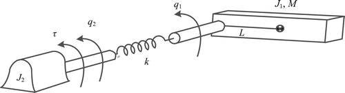
4.2. Example 2. Under-actuated systems

Consider a robot system with elastic joints as shown in Figure 1. The dynamic model is given as (66) $\left\{\begin{array}{l}{J}_1{\ddot{q}}_1+D_1\left({\dot{q}}_1\right){\dot{q}}_1+k{q}_1-k{q}_2=d_1\\ J_2{\ddot{q}}_2+D_2{\dot{q}}_2+k{q}_2-k{q}_1=\tau +d_2\\ \dot{\tau }=\varphi \left(\tau \right)+u+d_3,\end{array}\right.$(66) where the variables are defined as follows: $\begin{array}{ll}{q}_i,i=1,2& \text{angle of two joints;}\\ J_i,i=1,2& \text{moments of inertia of joints;}\\ D_i,i=1,2& \text{generalised joint damping;}\\ k& \text{spring stiffness;}\\ \tau & \text{output torque of the motor;}\\ u& \text{voltage input of the motor;}\\ d_i,i=1,2,3& \text{disturbance signals; and}\\ \varphi \left(t\right)& \text{piecewise continuous function.}\end{array}$ If we let (67) $\begin{array}{rl}& \left[\begin{array}{l}{x}_1\\ x_2\\ x_3\end{array}\right]=\left[\begin{array}{l}{q}_1\\ q_2\\ \tau \end{array}\right],\\ & \left\{\begin{array}{l}{f}_1=-\frac{1}{J_1}\left[D_1\right({\dot{x}}_1){\dot{x}}_1+k{x}_1]+d_1\\ f_2=-\frac{1}{J_2}\left[D_2\right({\dot{x}}_2){\dot{x}}_2+k{x}_2-k{x}_1]+d_2\\ f_3=\varphi \left(x_3\right)+d_3,\end{array}\right.\\ & G_1=k,G_2=\frac{1}{J_2},G_3=1,\end{array}$(67) then the system (66(66) $\left\{\begin{array}{l}{J}_1{\ddot{q}}_1+D_1\left({\dot{q}}_1\right){\dot{q}}_1+k{q}_1-k{q}_2=d_1\\ J_2{\ddot{q}}_2+D_2{\dot{q}}_2+k{q}_2-k{q}_1=\tau +d_2\\ \dot{\tau }=\varphi \left(\tau \right)+u+d_3,\end{array}\right.$(66) ) is clearly an SFS in the form of (18(18) $\left\{\begin{array}{l}{x}_1^{\left(m_1\right)}=f_1(x_1^{(0\sim m_1-1)},\zeta ,t)+G_1(x_1^{(0\sim m_1-1)},\zeta ,t)x_2\\ x_2^{\left(m_2\right)}=f_2(x_1^{(0\sim m_1)},x_2^{(0\sim m_2-1)},\zeta ,t)\\ +G_2(x_1^{(0\sim m_1)},x_2^{(0\sim m_2-1)},\zeta ,t)x_3\\ ⋮\\ x_n^{\left(m_n\right)}=f_n(x_i^{(0\sim m_i)}{|}_{i=1\sim n-1},x_n^{(0\sim m_n-1)},\zeta ,t)\\ +G_n(x_i^{(0\sim m_i)}{|}_{i=1\sim n-1},x_n^{(0\sim m_n-1)},\zeta ,t)u,\end{array}\right.$(18) ), which corresponds to the case of $n=3,\mathrm{a}\mathrm{n}\mathrm{d}{m}_1=m_2=2,m_3=1.$ Thus we have $p_1=2,p_2=4,\mathrm{a}\mathrm{n}\mathrm{d}p=p_3=5.$ Therefore, Theorem 2.3 or 3.4 can be readily applied to solve the problem. However, in order to support the point that many systems can really be physically modelled as a HOFA model instead of a state-space one, in the following we directly operate on the system (66(66) $\left\{\begin{array}{l}{J}_1{\ddot{q}}_1+D_1\left({\dot{q}}_1\right){\dot{q}}_1+k{q}_1-k{q}_2=d_1\\ J_2{\ddot{q}}_2+D_2{\dot{q}}_2+k{q}_2-k{q}_1=\tau +d_2\\ \dot{\tau }=\varphi \left(\tau \right)+u+d_3,\end{array}\right.$(66) ) based on the idea shown in the proof of Theorem 2.3, rather than applying the formulas directly.

Taking the second-order derivatives of both sides of the first equation in (66(66) $\left\{\begin{array}{l}{J}_1{\ddot{q}}_1+D_1\left({\dot{q}}_1\right){\dot{q}}_1+k{q}_1-k{q}_2=d_1\\ J_2{\ddot{q}}_2+D_2{\dot{q}}_2+k{q}_2-k{q}_1=\tau +d_2\\ \dot{\tau }=\varphi \left(\tau \right)+u+d_3,\end{array}\right.$(66) ), gives (68) $\begin{array}{rl}& J_1{q}_1^{\left(4\right)}+D_1\left({\dot{q}}_1\right)\stackrel{⃛}{q}{}_1+\left[2{\dot{D}}_1\right({\dot{q}}_1)+k]{\ddot{q}}_1\\ & +{\ddot{D}}_1\left({\dot{q}}_1\right){\dot{q}}_1-k{\ddot{q}}_2={\ddot{d}}_1.\end{array}$(68) It follows from the first equation in (66(66) $\left\{\begin{array}{l}{J}_1{\ddot{q}}_1+D_1\left({\dot{q}}_1\right){\dot{q}}_1+k{q}_1-k{q}_2=d_1\\ J_2{\ddot{q}}_2+D_2{\dot{q}}_2+k{q}_2-k{q}_1=\tau +d_2\\ \dot{\tau }=\varphi \left(\tau \right)+u+d_3,\end{array}\right.$(66) ) that (69) $q_2=\frac{1}{k}[J_1{\ddot{q}}_1+D_1({\dot{q}}_1){\dot{q}}_1-d_1]+q_1,$(69) which further gives (70) ${\dot{q}}_2=\frac{1}{k}\left[{J_1\stackrel{⃛}{q}}_1+D_1\left({\dot{q}}_1\right){\ddot{q}}_1+{\dot{D}}_1\left({\dot{q}}_1\right){\dot{q}}_1-{\dot{d}}_1\right]+{\dot{q}}_1.$(70) It follows from the second equation in (66(66) $\left\{\begin{array}{l}{J}_1{\ddot{q}}_1+D_1\left({\dot{q}}_1\right){\dot{q}}_1+k{q}_1-k{q}_2=d_1\\ J_2{\ddot{q}}_2+D_2{\dot{q}}_2+k{q}_2-k{q}_1=\tau +d_2\\ \dot{\tau }=\varphi \left(\tau \right)+u+d_3,\end{array}\right.$(66) ) that (71) ${\ddot{q}}_2=-\frac{1}{J_2}[D_2{\dot{q}}_2+k{q}_2-k{q}_1-\tau -d_2].$(71) Substituting (69(69) $q_2=\frac{1}{k}[J_1{\ddot{q}}_1+D_1({\dot{q}}_1){\dot{q}}_1-d_1]+q_1,$(69) ) and (70(70) ${\dot{q}}_2=\frac{1}{k}\left[{J_1\stackrel{⃛}{q}}_1+D_1\left({\dot{q}}_1\right){\ddot{q}}_1+{\dot{D}}_1\left({\dot{q}}_1\right){\dot{q}}_1-{\dot{d}}_1\right]+{\dot{q}}_1.$(70) ) into the above Equation (71(71) ${\ddot{q}}_2=-\frac{1}{J_2}[D_2{\dot{q}}_2+k{q}_2-k{q}_1-\tau -d_2].$(71) ), gives the following form of ${\ddot{q}}_2$ expressed only by $q_1$ and its derivatives: (72) $\begin{array}{rl}{\ddot{q}}_2& =-\frac{1}{k{J}_2}{D}_2\left[{J_1\stackrel{⃛}{q}}_1+D_1\left({\dot{q}}_1\right){\ddot{q}}_1+{\dot{D}}_1\left({\dot{q}}_1\right){\dot{q}}_1-{\dot{d}}_1\right]\\ & -\frac{1}{J_2}\left[D_2{\dot{q}}_1+J_1{\ddot{q}}_1+D_1\left({\dot{q}}_1\right){\dot{q}}_1-\tau -d_1-d_2\right].\end{array}$(72) Further, substituting the above equation into (68(68) $\begin{array}{rl}& J_1{q}_1^{\left(4\right)}+D_1\left({\dot{q}}_1\right)\stackrel{⃛}{q}{}_1+\left[2{\dot{D}}_1\right({\dot{q}}_1)+k]{\ddot{q}}_1\\ & +{\ddot{D}}_1\left({\dot{q}}_1\right){\dot{q}}_1-k{\ddot{q}}_2={\ddot{d}}_1.\end{array}$(68) ), yields the following fourth-order fully-actuated quasi-linear system: (73) $J_2{J}_1{q}_1^{\left(4\right)}+\sum _{i=1}^3{c}_i\left(q_1^{(1\sim 3)}\right)q_1^{\left(i\right)}=k\tau +\hat{d},$(73) where (74) $\left\{\begin{array}{l}{c}_1\left(q_1^{(1\sim 3)}\right)=J_2{\ddot{D}}_1\left({\dot{q}}_1\right)+D_2\left({\dot{D}}_1\left({\dot{q}}_1\right)+k\right)+k{D}_1\left({\dot{q}}_1\right)\\ c_2\left(q_1^{(1\sim 3)}\right)=2J_2{\dot{D}}_1\left({\dot{q}}_1\right)+D_2{D}_1\left({\dot{q}}_1\right)+(J_1+J_2)k\\ c_3\left({\dot{q}}_1\right)=J_2{D}_1\left({\dot{q}}_1\right)+J_1{D}_2,\end{array}\right.$(74) and (75) $\hat{d}=k(d_1+d_2)+D_2{\dot{d}}_1+J_2{\ddot{d}}_1.$(75) Finally, taking the derivatives of both sides of (73(73) $J_2{J}_1{q}_1^{\left(4\right)}+\sum _{i=1}^3{c}_i\left(q_1^{(1\sim 3)}\right)q_1^{\left(i\right)}=k\tau +\hat{d},$(73) ), and substituting the last equation in (66(66) $\left\{\begin{array}{l}{J}_1{\ddot{q}}_1+D_1\left({\dot{q}}_1\right){\dot{q}}_1+k{q}_1-k{q}_2=d_1\\ J_2{\ddot{q}}_2+D_2{\dot{q}}_2+k{q}_2-k{q}_1=\tau +d_2\\ \dot{\tau }=\varphi \left(\tau \right)+u+d_3,\end{array}\right.$(66) ) into the result, give the following fifth-order fully-actuated quasi-linear system (76) $J_2{J}_1{q}_1^{\left(5\right)}+\sum _{i=0}^4{a}_i\left(q_1^{(1\sim 4)}\right)q_1^{\left(i\right)}-k\varphi \left(\tau \right)=ku+kd,$(76) where (77) $\left\{\begin{array}{l}{a}_0=0\\ a_1\left(q_1^{(1\sim 4)}\right)={\dot{c}}_1\left(q_1^{(1\sim 3)}\right)\\ a_2\left(q_1^{(1\sim 4)}\right)={\dot{c}}_2\left(q_1^{(1\sim 3)}\right)+c_1\left(q_1^{(1\sim 3)}\right)\\ a_3\left(q_1^{(1\sim 4)}\right)={\dot{c}}_3\left({\dot{q}}_1\right)+c_2\left(q_1^{(1\sim 3)}\right)\\ a_4\left({\dot{q}}_1\right)=c_3\left({\dot{q}}_1\right),\end{array}\right.$(77) and (78) $d=k({\dot{d}}_1+{\dot{d}}_2+d_3)+D_2{\ddot{d}}_1+J_2{\stackrel{⃛}{d}}_1,$(78) with $c_i\left(q_1^{(1\sim 3)}\right),i=1,2,3$ being given by (74(74) $\left\{\begin{array}{l}{c}_1\left(q_1^{(1\sim 3)}\right)=J_2{\ddot{D}}_1\left({\dot{q}}_1\right)+D_2\left({\dot{D}}_1\left({\dot{q}}_1\right)+k\right)+k{D}_1\left({\dot{q}}_1\right)\\ c_2\left(q_1^{(1\sim 3)}\right)=2J_2{\dot{D}}_1\left({\dot{q}}_1\right)+D_2{D}_1\left({\dot{q}}_1\right)+(J_1+J_2)k\\ c_3\left({\dot{q}}_1\right)=J_2{D}_1\left({\dot{q}}_1\right)+J_1{D}_2,\end{array}\right.$(74) ).

When the state variables $q_1,q_2,{\dot{q}}_1,{\dot{q}}_2,$ and τ of all the subsystems of the original system (66(66) $\left\{\begin{array}{l}{J}_1{\ddot{q}}_1+D_1\left({\dot{q}}_1\right){\dot{q}}_1+k{q}_1-k{q}_2=d_1\\ J_2{\ddot{q}}_2+D_2{\dot{q}}_2+k{q}_2-k{q}_1=\tau +d_2\\ \dot{\tau }=\varphi \left(\tau \right)+u+d_3,\end{array}\right.$(66) ) are all measurable, it is easy to obtain the state $q_1^{(0\sim 4)}$ of the system (76(76) $J_2{J}_1{q}_1^{\left(5\right)}+\sum _{i=0}^4{a}_i\left(q_1^{(1\sim 4)}\right)q_1^{\left(i\right)}-k\varphi \left(\tau \right)=ku+kd,$(76) ), thus we can design the following state feedback control law for the system (76(76) $J_2{J}_1{q}_1^{\left(5\right)}+\sum _{i=0}^4{a}_i\left(q_1^{(1\sim 4)}\right)q_1^{\left(i\right)}-k\varphi \left(\tau \right)=ku+kd,$(76) ): (79) $\begin{array}{rl}u& =\frac{1}{k}\sum _{i=0}^4\left[a_i\left(q_1^{(1\sim 4)}\right)-J_1{J}_2{\alpha }_i\right]q_1^{\left(i\right)}\\ & +\frac{1}{k}{J}_1{J}_{2}v-\varphi \left(\tau \right),\end{array}$(79) where ${\alpha }_i,i=0\sim 4$ are a set of parameters, v is the reference input. Under the above control law, the following linear closed-loop system can be obtained: (80) $q_1^{\left(5\right)}+\sum _{i=0}^4{\alpha }_i{q}_1^{\left(i\right)}=v+\frac{k}{J_1{J}_2}d.$(80) Since the above system is a single variable one, the design parameters ${\alpha }_i,i=0\sim 4$ are uniquely determined by the closed-loop poles of the system. Therefore, the design parameters ${\alpha }_i,i=0\sim 4$ can be designed by making proper choice of the closed-loop poles.

Figure 1. A robot system with elastic joints.

When the disturbance signals $d_i,i=1,2$ are constant ones, it follows from (78(78) $d=k({\dot{d}}_1+{\dot{d}}_2+d_3)+D_2{\ddot{d}}_1+J_2{\stackrel{⃛}{d}}_1,$(78) ) that the above design through the HOFA model (80(80) $q_1^{\left(5\right)}+\sum _{i=0}^4{\alpha }_i{q}_1^{\left(i\right)}=v+\frac{k}{J_1{J}_2}d.$(80) ) has simultaneously achieved decoupling of the disturbance signals $d_1$ and $d_2$. When the disturbance $d_1$ is a ramp signal, only its slope has an affection to the HOFA system (80(80) $q_1^{\left(5\right)}+\sum _{i=0}^4{\alpha }_i{q}_1^{\left(i\right)}=v+\frac{k}{J_1{J}_2}d.$(80) ). Even if for the case that the disturbances are all general signals, the problem still gets simplified since in the high-order system all the individual disturbance signals are assembled into a comprehensive one, and the problem is then turned into one of disturbance attenuation in the constant linear system (80(80) $q_1^{\left(5\right)}+\sum _{i=0}^4{\alpha }_i{q}_1^{\left(i\right)}=v+\frac{k}{J_1{J}_2}d.$(80) ).

Remark 4.1

It is clearly seen from the above two examples that the solution processes of the HOFA system approach are very simple. If the first example system is converted into a first-order system with two multivariable subsystems, and the second example system is converted into a first order system with 5 subsystems, experience tells us that applications of method of backsteppinig to the converted first-order systems should turn out to be much more complicated.

5. Conclusion

The HOFA system approach is very powerful in dealing with the control of nonlinear systems, since the full-actuation feature allows one to eliminate the nonlinearities and hence a constant linear closed-loop system can be obtained. To apply the HOFA approach, the key step is to obtain a HOFA model for a nonlinear system. Toward this goal, this paper has shown the following:

1. The conventional SFS can be further generalised to contain parameter vectors and the derivatives of the state vectors, and a recursive solution exists to convert the generalised version of SFS equivalently into a HOFA model;

2. due to the fact that second- and high-order subsystems are firstly obtained when modelling using physical laws such as Newton's law, Lagrangian equation, Theorem of linear and angular momentum, Kirchhoff's law of current and voltage, etc., the proposed SFSs of second-order, and that with subsystems of mixed orders are much more commonly encountered than the first-order ones;

3. like the first-order case, effective recursive solutions also exist for converting the proposed second-order or mixed-order SFSs equivalently into HOFA models; and

4. under certain common conditions, the recursive solutions to convert the proposed generalised SFSs equivalently into HOFA models can be expressed in direct analytical explicit forms.

The above facts are very important since they partially provide a base of the effective HOFA approach for control of generalised complicated strict-feedback nonlinear systems, which may be no longer effectively solved with the well-known method of backstepping due to more serious ‘differential explosion’ problems caused by the increased complexity in the proposed generalised SFSs.

Acknowledgements

The author is grateful to his Ph.D. students, Tianyi Zhao, Yanmei Hu, Qin Zhao, Guangtai Tian, Yajun Gao, etc., for helping him with reference selection and proofreading.

Disclosure statement

No potential conflict of interest was reported by the author(s).

Correction Statement

This article has been republished with minor changes. These changes do not impact the academic content of the article.

Additional information

Funding

This work has been partially supported by the Major Program of National Natural Science Foundation of China [grant numbers 61690210, 61690212], the National Natural Science Foundation of China [grant number 61333003] and the Self-Planned Task of State Key Laboratory of Robotics and System (HIT) [grant number SKLRS201716A].

Notes on contributors

Guangren Duan

Guangren Duan received his Ph.D. degree in Control Systems Sciences from Harbin Institute of Technology, Harbin, P. R. China, in 1989. After a two-year post-doctoral experince at the same university, he became professor of control systems theory at that university in 1991. He is the founder and currently the Director of the Center for Control Theory and Guidance Technology at Harbin Institute of Technology. He visited the University of Hull, the University of Sheffield, and also the Queen's University of Belfast, UK, from December 1996 to October 2002, and has served as Member of the Science and Technology committee of the Chinese Ministry of Education, Vice President of the Control Theory and Applications Committee, Chinese Association of Automation (CAA), and Associate Editors of a few international journals. He is currently an Academician of the Chinese Academy of sciences, and Fellow of CAA, IEEE and IET. His main research interests include parametric control systems design, nonlinear systems, descriptor systems, spacecraft control and magnetic bearing control. He is the author and co-author of 5 books and over 270 SCI indexed publications.

Appendix.

Proofs of Theorems 2.1–2.3

A.1. Proof of Theorem 2.1

We use mathematical induction to prove this result.

Firstly, let us consider the case of n = 2. In this case, the system is (81) $\left\{\begin{array}{l}{\dot{x}}_1=f_1(x_1,\zeta ,t)+G_1(x_1,\zeta ,t)x_2\\ {\dot{x}}_2=f_2(x_1^{(0\sim 1)},x_2,\zeta ,t)+G_2(x_1^{(0\sim 1)},x_2,\zeta ,t)u.\end{array}\right.$(81) It follows from the first equation in (A1) that (82) $x_2=G_1^{-1}(x_1,\zeta ,t)[{\dot{x}}_1-f_1(x_1,\zeta ,t\left)\right],$(82) which gives the following transformation (83) $\left\{\begin{array}{l}{x}_1=z\\ x_2=G_1^{-1}(z,\zeta ,t)[\dot{z}-f_1(z,\zeta ,t\left)\right].\end{array}\right.$(83) Next, taking the derivatives of both sides of the first equation in (A1), and substituting the second one into the result, give (84) $\begin{array}{rl}{\ddot{x}}_1& ={\dot{f}}_1(x_1,\zeta ,t)+{\dot{G}}_1(x_1,\zeta ,t)x_2\\ & +G_1(x_1,\zeta ,t)f_2(x_1^{(0\sim 1)},x_2,\zeta ,t)\\ & +G_1(x_1,\zeta ,t)G_2(x_1^{(0\sim 1)},x_2,\zeta ,t)u.\end{array}$(84) Further, substituting (A3) into the above equation, produces the following second-order fully-actuated system (85) $\ddot{z}=h_2\left(z^{(0\sim 1)},\zeta ,t\right)+L_2\left(z^{(0\sim 1)},\zeta ,t\right)u,$(85) where (86) $\begin{array}{rl}{L}_2\left(z^{(0\sim 1)},\zeta ,t\right)& =G_1(z,\zeta ,t)G_2(z^{(0\sim 1)},x_2,\zeta ,t),\end{array}$(86) (87) $\begin{array}{rl}{h}_2\left(z^{(0\sim 1)},\zeta ,t\right)& ={\dot{f}}_1(z,\zeta ,t)+{\dot{G}}_1(z,\zeta ,t)x_2\\ & +G_1(z,\zeta ,t)f_2(z^{(0\sim 1)},x_2,\zeta ,t),\end{array}$(87) and the variable $x_2$ in the above two equations should be substituted by the second equation in (A3). In view of $h_1(z,\zeta ,t)=f_1(z,\zeta ,t)$ and $L_1(z,\zeta ,t)=G_1(z,\zeta ,t)$, the above (A7) gives the formula (8(8) $\begin{array}{rl}& h_k(z^{(0\sim k-1)},\zeta ,t)\\ & ={\dot{h}}_{k-1}(z^{(0\sim k-2)},\zeta ,t)+{\dot{L}}_{k-1}(z^{(0\sim k-2)},\zeta ,t)x_k\\ & +L_{k-1}(z^{(0\sim k-2)},\zeta ,t)f_k(x_{1\sim k-1}^{(0\sim 1)},x_k,\zeta ,t),\\ & k=1,2,\dots ,n\end{array}$(8) ) for the case of n = 2.

Finally, recalling the nonsingularity of $G_1(z,\zeta ,t)$ and $G_2(z^{(0\sim 1)},x_2,\zeta ,t)$, and the definition of $L_2(z^{(0\sim 1)},\zeta ,t)$, we know that the system (A5) is fully-actuated, thus the theorem holds in the case of n = 2.

Now let us assume that the theorem holds when n = k. For convenience, we still denote u as $x_{k+1}$. In this case the system takes the form of (88) $\left\{\begin{array}{l}{\dot{x}}_1=f_1(x_1,\zeta ,t)+G_1(x_1,\zeta ,t)x_2\\ {\dot{x}}_2=f_2(x_1^{(0\sim 1)},x_2,\zeta ,t)+G_2(x_1^{(0\sim 1)},x_2,\zeta ,t)x_3\\ ⋮\\ {\dot{x}}_k=f_k(x_{1\sim k-1}^{(0\sim 1)},x_k,\zeta ,t)+G_k(x_{1\sim k-1}^{(0\sim 1)},x_k,\zeta ,t)x_{k+1},\end{array}\right.$(88) which, under the following transformation, (89) $\left\{\begin{array}{l}{x}_1=z\\ x_2=G_1^{-1}(z,\zeta ,t)[\dot{z}-f_1(z,\zeta ,t\left)\right]\\ x_{i+1}=L_i^{-1}(z^{(0\sim i-1)},\zeta ,t)[z^{\left(i\right)}-h_i(z^{(0\sim i-1)},\zeta ,t\left)\right],\\ i=2,3,\dots ,k-1,\end{array}\right.$(89) can be expressed as the following high-order system form (90) $z^{\left(k\right)}=h_k(z^{(0\sim k-1)},\zeta ,t)+L_k(z^{(0\sim k-1)},\zeta ,t)x_{k+1},$(90) where (91) $\begin{array}{rl}& L_k(z^{(0\sim k-1)},\zeta ,t)\\ & =G_1(z,\zeta ,t)G_2(z^{(0\sim 1)},x_2,\zeta ,t)\cdots G_k(x_{1\sim k-1}^{(0\sim 1)},x_k,\zeta ,t).\end{array}$(91) Now let us prove the conclusion for the case of n = k + 1.

When n = k + 1, noting that the first k formulas of the system are exactly the system (A8), we know from the assumption that the system can be equivalently rewritten as (92) $\left\{\begin{array}{l}{z}^{\left(k\right)}=h_k(z^{(0\sim k-1)},\zeta ,t)+L_k(z^{(0\sim k-1)},\zeta ,t)x_{k+1}\\ {\dot{x}}_{k+1}=f_{k+1}(x_{1\sim k}^{(0\sim 1)},x_{k+1},\zeta ,t)+G_{k+1}(x_{1\sim k}^{(0\sim 1)},x_{k+1},\zeta ,t)u.\end{array}\right.$(92) It follows from the first equation in (A12) that (93) $x_{k+1}=L_k^{-1}(z^{(0\sim k-1)},\zeta ,t)[x_1^{\left(k\right)}-h_k(z^{(0\sim k-1)},\zeta ,t\left)\right].$(93) Combining (A13) with (A9), gives the following transformation (94) $\left\{\begin{array}{l}{x}_1=z\\ x_2=G_1^{-1}(z,\zeta ,t)[\dot{z}-f_1(z,\zeta ,t\left)\right]\\ x_{i+1}=L_i^{-1}(z^{(0\sim i-1)},\zeta ,t)[z^{\left(i\right)}-h_i(z^{(0\sim i-1)},\zeta ,t\left)\right],\\ i=2,3,\dots ,k.\end{array}\right.$(94) Further, taking the derivatives of both sides of the first equation in (A12), and then substituting the second one, give (95) $\begin{array}{rl}{z}^{(k+1)}& ={\dot{h}}_k(z^{(0\sim k-1)},\zeta ,t)+{\dot{L}}_k(z^{(0\sim k-1)},\zeta ,t)x_{k+1}\\ & +L_k(z^{(0\sim k-1)},\zeta ,t)f_{k+1}(x_{1\sim k}^{(0\sim 1)},x_{k+1},\zeta ,t)\\ & +L_k(z^{(0\sim k-1)},\zeta ,t)G_{k+1}(x_{1\sim k}^{(0\sim 1)},x_{k+1},\zeta ,t)u.\end{array}$(95) Then, substituting (A14) and its derivative into (A15), yields the following high-order system (96) $z^{\left(k+1\right)}=h_{k+1}(z^{(0\sim k)},\zeta ,t)+L_{k+1}(z^{(0\sim k)},\zeta ,t)u,$(96) where (97) $\begin{array}{rl}& L_{k+1}(z^{(0\sim k)},\zeta ,t)\\ & =L_k(z^{(0\sim k-1)},\zeta ,t)G_{k+1}(x_{1\sim k}^{(0\sim 1)},x_{k+1},\zeta ,t)\\ & =G_1(x_1,\zeta ,t)G_2(x_1,{\dot{x}}_1,x_2,\zeta ,t)\cdots G_{k+1}(x_{1\sim k}^{(0\sim 1)},x_{k+1},\zeta ,t),\end{array}$(97) with $h_{k+1}(z^{(0\sim k)},\zeta ,t)$ being given by (8(8) $\begin{array}{rl}& h_k(z^{(0\sim k-1)},\zeta ,t)\\ & ={\dot{h}}_{k-1}(z^{(0\sim k-2)},\zeta ,t)+{\dot{L}}_{k-1}(z^{(0\sim k-2)},\zeta ,t)x_k\\ & +L_{k-1}(z^{(0\sim k-2)},\zeta ,t)f_k(x_{1\sim k-1}^{(0\sim 1)},x_k,\zeta ,t),\\ & k=1,2,\dots ,n\end{array}$(8) ).

Finally, it is known from the nonsingularity of $G_k(x_{1\sim k-1}^{(0\sim 1)},x_k,\zeta ,t),k=1,2,\dots ,n$ and the definitions of the above $L_{k+1}(z^{(0\sim k)},\zeta ,t)$ that the system (A16) is fully-actuated. Thus the theorem also holds in the case of n = k + 1. Therefore, the whole proof is completed.

A.2. Proof of Theorem 2.2

Again we prove this result using mathematical induction.

Let us firstly consider the case of n = 2. For convenience, we still use the notation $x_3$ in the position of u, in this case the system is (98) $\left\{\begin{array}{l}{\ddot{x}}_1=f_1(x_1^{(0\sim 1)},\zeta ,t)+G_1(x_1^{(0\sim 1)},\zeta ,t)x_2\\ {\ddot{x}}_2=f_2(x_1^{(0\sim 2)},x_2^{(0\sim 1)},\zeta ,t)+G_2(x_1^{(0\sim 2)},x_2^{(0\sim 1)},\zeta ,t)x_3.\end{array}\right.$(98) It follows from the first equation in (A18) that (99) $x_2=G_1^{-1}(x_1^{(0\sim 1)},\zeta ,t)[{\ddot{x}}_1-f_1(x_1^{(0\sim 1)},\zeta ,t\left)\right].$(99) Thus the following transformation can be obtained (100) $\left\{\begin{array}{l}{x}_1=z\\ x_2=G_1^{-1}(z^{(0\sim 1)},\zeta ,t)[\ddot{z}-f_1(z^{(0\sim 1)},\zeta ,t\left)\right],\end{array}\right.$(100) which gives (101) $\left\{\begin{array}{l}{\dot{x}}_1=\dot{z}\\ {\dot{x}}_2\stackrel{\mathrm{\Delta }}{=}{d}_1^{x2}(z^{(0\sim 3)},\zeta ,t),\end{array}\right.$(101) with $\begin{array}{rl}& d_1^{x2}(z^{(0\sim 3)},\zeta ,t)\\ & ={\left[G_1^{-1}(z^{(0\sim 1)},\zeta ,t)\right]}^{\mathrm{\prime }}[\ddot{z}-f_1(z^{(0\sim 1)},\zeta ,t\left)\right]\\ & +G_1^{-1}(z^{(0\sim 1)},\zeta ,t)[\stackrel{⃛}{z}-{\dot{f}}_1(z^{(0\sim 1)},\zeta ,t\left)\right].\end{array}$ Next, taking the second-order derivatives of both sides of the first equation in (A18), and then substituting the second equation in (A18) into the result, give (102) $\begin{array}{rl}{z}^{\left(4\right)}& ={\ddot{f}}_1(z^{(0\sim 1)},\zeta ,t)+{\ddot{G}}_1(z^{(0\sim 1)},\zeta ,t)x_2+2{\dot{G}}_1(z^{(0\sim 1)},\zeta ,t){\dot{x}}_2\\ & +G_1(z^{(0\sim 1)},\zeta ,t)f_2(z^{(0\sim 2)},x_2^{(0\sim 1)},\zeta ,t)\\ & +G_1(z^{(0\sim 1)},\zeta ,t)G_2(z^{(0\sim 2)},x_2^{(0\sim 1)},\zeta ,t)x_3.\end{array}$(102) Further, substituting (A20) and (A21) into the above equation, yields the following fourth-order system (103) $z^{\left(4\right)}=h_2(z^{(0\sim 3)},\zeta ,t)+L_2(z^{(0\sim 3)},\zeta ,t)x_3,$(103) where (104) $L_2(z^{(0\sim 3)},\zeta ,t)=G_1(x_1^{(0\sim 1)},\zeta ,t)G_2(x_1^{(0\sim 2)},x_2^{(0\sim 1)},\zeta ,t),$(104) and (105) $\begin{array}{rl}& h_2(z^{(0\sim 3)},\zeta ,t)\\ & ={\ddot{f}}_1(z^{(0\sim 1)},\zeta ,t)+{\ddot{G}}_1(z^{(0\sim 1)},\zeta ,t)x_2+2{\dot{G}}_1(z^{(0\sim 1)},\zeta ,t){\dot{x}}_2\\ & +G_1(z^{(0\sim 1)},\zeta ,t)f_2(x_1^{(0\sim 2)},x_2^{(0\sim 1)},\zeta ,t),\end{array}$(105) and the variable $x_2$ and its derivative in the above equation are substituted with (A20) and (A21). Recalling that $h_1(z^{(0\sim 1)},\zeta ,t)=f_1(z^{(0\sim 1)},\zeta ,t)$ and $L_1(z^{(0\sim 1)},\zeta ,t)=G_1(z^{(0\sim 1)},\zeta ,t)$, we know that the above (A25) gives the formula (47(47) $z^{\left(p\right)}=h_n(z^{(0\sim p-1)},\zeta ,t)+L_n(z^{(0\sim p-1)},\zeta ,t)u,$(47) ) for the case of n = 2.

Finally, in view of the nonsingularity of $G_1(z^{(0\sim 1)},\zeta ,t)$ and $G_2(z^{(0\sim 2)},x_2^{(0\sim 1)},\zeta ,t)$, and the definition of $L_2(z^{(0\sim 3)},\zeta ,t)$ above, the system (A23) is easily seen to be fully-actuated. Thus the theorem holds when n = 2.

Now assume that the theorem holds when n = k. For convenience, we still denote u as $x_{k+1}$, in this case the system is (106) $\left\{\begin{array}{l}{\ddot{x}}_1=f_1(x_1^{(0\sim 1)},\zeta ,t)+G_1(x_1^{(0\sim 1)},\zeta ,t)x_2\\ {\ddot{x}}_2=f_2(x_1^{(0\sim 2)},x_2^{(0\sim 1)},\zeta ,t)+G_2(x_1^{(0\sim 2)},x_2^{(0\sim 1)},\zeta ,t)x_3\\ ⋮\\ {\ddot{x}}_k=f_k(x_{1\sim k-1}^{(0\sim 2)},x_k^{(0\sim 1)},\zeta ,t)+G_k(x_{1\sim k-1}^{(0\sim 2)},x_k^{(0\sim 1)},\zeta ,t)x_{k+1},\end{array}\right.$(106) which, under the following transformation, (107) $\left\{\begin{array}{l}{x}_1=z\\ x_2=G_1^{-1}(z^{(0\sim 1)},\zeta ,t)[\ddot{z}-f_1(z^{(0\sim 1)},\zeta ,t\left)\right]\\ x_{i+1}=L_i^{-1}(z^{(0\sim 2i-1)},\zeta ,t)[z^{\left(2i\right)}-h_i(z^{(0\sim 2i-1)},\zeta ,t\left)\right],\\ i=2,3,\dots ,k-1,\end{array}\right.$(107) can be rewritten into (108) $z^{\left(2k\right)}=h_k(z^{(0\sim 2k-1)},\zeta ,t)+L_k(z^{(0\sim 2k-1)},\zeta ,t)x_{k+1},$(108) where (109) $\begin{array}{rl}& L_k(z^{(0\sim 2k-1)},\zeta ,t)\\ & =L_{k-1}(z^{(0\sim 2k-2)},\zeta ,t)G_k(x_{1\sim k-1}^{(0\sim 2)},x_k^{(0\sim 1)},\zeta ,t).\end{array}$(109) Let us now prove the conclusion for the case of n = k + 1.

When n = k + 1, it is easy to know that the first k equations of the system are exactly the system (A26). Thus it is known from the assumptions that in this case the system can be expressed as (110) $\left\{\begin{array}{l}{z}^{\left(2k\right)}=h_k(z^{(0\sim 2k-1)},\zeta ,t)+L_k(z^{(0\sim 2k-1)},\zeta ,t)x_{k+1}\\ {\ddot{x}}_{k+1}=f_{k+1}(x_{1\sim k}^{(0\sim 2)},x_{k+1}^{(0\sim 1)},\zeta ,t)+G_{k+1}(x_{1\sim k}^{(0\sim 2)},x_{k+1}^{(0\sim 1)},\zeta ,t)u.\end{array}\right.$(110) It follows from the first equation in (A30) that (111) $x_{k+1}=L_k^{-1}(z^{(0\sim 2k-1)},\zeta ,t)[z^{\left(2k\right)}-h_k(z^{(0\sim 2k-1)},\zeta ,t\left)\right].$(111) Combining the above equation with (A27), yields (112) $\left\{\begin{array}{l}{x}_1=z\\ x_2=G_1^{-1}(z^{(0\sim 1)},\zeta ,t)[\ddot{z}-f_1(z^{(0\sim 1)},\zeta ,t\left)\right]\\ x_{i+1}=L_i^{-1}(z^{(0\sim 2i-1)},\zeta ,t)[z^{\left(2i\right)}-h_i(z^{(0\sim 2i-1)},\zeta ,t\left)\right],\\ i=2,3,\dots ,k.\end{array}\right.$(112) Taking the second-order derivatives of both sides of the first equation in (A30), and then substituting the second one into the result, give (113) $\begin{array}{rl}{z}^{(2k+2)}& ={\ddot{h}}_k(z^{(0\sim 2k-1)},\zeta ,t)+{\ddot{L}}_k(z^{(0\sim 2k-1)},\zeta ,t)x_{k+1}\\ & +2{\dot{L}}_k(z^{(0\sim 2k-1)},\zeta ,t){\dot{x}}_{k+1}\\ & +L_k(z^{(0\sim 2k-1)},\zeta ,t)f_{k+1}(x_{1\sim k}^{(0\sim 2)},x_{k+1}^{(0\sim 1)},\zeta ,t)\\ & +L_k(z^{(0\sim 2k-1)},\zeta ,t)G_{k+1}(x_{1\sim k}^{(0\sim 2)},x_{k+1}^{(0\sim 1)},\zeta ,t)u,\end{array}$(113) where $x_i,i=2,3,\dots ,k$ and their derivatives are given by (A32). Taking (114) $\begin{array}{rl}& L_{k+1}(z^{(0\sim 2k+1)},\zeta ,t)\\ & =L_k(z^{(0\sim 2k-1)},\zeta ,t)G_{k+1}(x_{1\sim k}^{(0\sim 2)},x_{k+1}^{(0\sim 1)},\zeta ,t),\end{array}$(114) and $h_{k+1}(z^{(0\sim 2k+1)},\zeta ,t)$ as in (47(47) $z^{\left(p\right)}=h_n(z^{(0\sim p-1)},\zeta ,t)+L_n(z^{(0\sim p-1)},\zeta ,t)u,$(47) ), the high-order system can be obtained as (115) $z^{(2k+2)}=h_{k+1}(z^{(0\sim 2k-1)},\zeta ,t)+L{}_{k+1}(z^{(0\sim 2k+1)},\zeta ,t)u.$(115) Finally, due to the nonsingularity of $G_k(x_{1\sim k-1}^{(0\sim 2)},x_k^{(0\sim 1)},\zeta ,t),k=1,2,\dots ,n$ and the above definitions of $L_{k+1}(z^{(0\sim 2k+1)},\zeta ,t)$, the system (A35) is clearly fully-actuated. Thus the theorem is also true in the case of n = k + 1. Therefore, the whole proof is completed.

A.3. Proof of Theorem 2.3

We again use mathematical induction to prove the result.

Firstly, let us consider the case of n = 2. Similarly, using the notation $x_3$ at the position of u, in this case the system is (116) $\left\{\begin{array}{l}{x}_1^{\left(m_1\right)}=f_1(x_1^{(0\sim m_1-1)},\zeta ,t)+G_1(x_1^{(0\sim m_1-1)},\zeta ,t)x_2\\ x_2^{\left(m_2\right)}=f_2(x_1^{(0\sim m_1)},x_2^{(0\sim m_2-1)},\zeta ,t)\\ +G_2(x_1^{(0\sim m_1)},x_2^{(0\sim m_2-1)},\zeta ,t)x_3.\end{array}\right.$(116) It follows from the first equation in (A36) that (117) $x_2=G_1^{-1}(x_1^{(0\sim m_1-1)},\zeta ,t)[x_1^{\left(m_1\right)}-f_1(x_1^{(0\sim m_1-1)},\zeta ,t\left)\right].$(117) Thus the following transformation can be obtained (118) $\left\{\begin{array}{l}{x}_1=z\\ x_2=G_1^{-1}(z^{(0\sim m_1-1)},\zeta ,t)[z^{\left(m_1\right)}-f_1(z^{(0\sim m_1-1)},\zeta ,t\left)\right],\end{array}\right.$(118) which further gives (119) $\left\{\begin{array}{l}{x}_1^{\left(i\right)}=z^{\left(i\right)},i=1\sim m_1-1\\ x_2^{\left(i\right)}\triangleq d_i^{x2}(z^{(0\sim m_1+i},\zeta ,t),i=1\sim m_2-1,\end{array}\right.$(119) with $\begin{array}{rl}& d_i^{x2}(z^{(0\sim m_1+i},\zeta ,t)\\ & ={\left[G_1^{-1}(z^{(0\sim m_1-1)},\zeta ,t)\right]}^{\mathrm{\prime }}[z^{\left(m_1\right)}-f_1(z^{(0\sim m_1-1)},\zeta ,t\left)\right]\\ & +G_1^{-1}(z^{(0\sim m_1-1)},\zeta ,t)[z^{\left(m_1+1\right)}-{\dot{f}}_1(z^{(0\sim m_1-1)},\zeta ,t\left)\right].\end{array}$ Taking the $m_2$-order derivatives of both sides of the first equation in (A36), and then substituting the second one into the result, give (120) $\begin{array}{rl}{x}_1^{\left(p_2\right)}& =f_1^{\left(m_2\right)}(x_1^{(0\sim m_1-1)},\zeta ,t)+\frac{{\mathrm{d}}^{m_2}}{\mathrm{d}{t}^{m_2}}\left[G_1\right(x_1^{(0\sim m_1-1)},\zeta ,t\left)x_2\right]\\ & =f_1^{\left(m_2\right)}(x_1^{(0\sim m_1-1)},\zeta ,t)\\ & +\sum _{k=0}^{m_2}C(k,n)G_1^{(m_2-k)}(x_1^{(0\sim m_1-1)},\zeta ,t)x_2^{\left(k\right)}\\ & =f_1^{\left(m_2\right)}(x_1^{(0\sim m_1-1)},\zeta ,t)\\ & +\sum _{k=0}^{m_2-1}C(k,n)G_1^{(m_2-k)}(x_1^{(0\sim m_1-1)},\zeta ,t)x_2^{\left(k\right)}\\ & +G_1(x_1^{(0\sim m_1-1)},\zeta ,t)\\ & \times \left[f_2(x_1^{(0\sim m_1)},x_2^{(0\sim m_2-1)},\zeta ,t)\right.\\ & +\left.G_2(x_1^{(0\sim m_1)},x_2^{(0\sim m_2-1)},\zeta ,t)u\right].\end{array}$(120) Further, substituting (A38) and (A39) into the above equation, produces the following high-order system (121) $z^{p_2}=h_2(z^{(0\sim p_2-1)},\zeta ,t)+L_2(z^{(0\sim p_2-1)},\zeta ,t)u,$(121) where (122) $\begin{array}{rl}& L_2(z^{(0\sim p_2-1)},\zeta ,t)\\ & =G_1(x_1^{(0\sim m_1-1)},\zeta ,t)G_2(x_1^{(0\sim m_1)},x_2^{(0\sim m_2-1)},\zeta ,t),\end{array}$(122) (123) $\begin{array}{rl}& h_2(z^{(0\sim p_2-1)},\zeta ,t)\\ & =f_1^{\left(m_2\right)}(x_1^{(0\sim m_1-1)},\zeta ,t)\\ & +\sum _{k=0}^{m_2-1}C(k,m_2)G_1^{(m_2-k)}(x_1^{(0\sim m_1-1)},\zeta ,t)x_2^{\left(k\right)}\\ & +G_1(x_1^{(0\sim m_1-1)},\zeta ,t)f_2(x_1^{(0\sim m_1)},x_2^{(0\sim m_2-1)},\zeta ,t).\end{array}$(123) Further, in view of $\begin{array}{rl}{h}_1(z^{(0\sim m_1-1)},\zeta ,t)& =f_1(z^{(0\sim m_1-1)},\zeta ,t),\\ L_1(z^{(0\sim m_1-1)},\zeta ,t)& =G_1(z^{(0\sim m_1-1)},\zeta ,t),\end{array}$ the above (A43) turns out to be (23(23) $\begin{array}{rl}& h_k(z^{(0\sim p_k-1)},\zeta ,t)\\ & =h_{k-1}^{(m_k)}(z^{(0\sim p_{k-1}-1)},\zeta ,t)\\ & +\sum _{j=0}^{m_k-1}C(j,m_k)L_{k-1}^{(m_k-j)}(z^{(0\sim p_{k-1}-1)},\zeta ,t)x_k^{\left(j\right)}\\ & +L_{k-1}(x_1^{(0\sim p_{k-1}-1)},\zeta ,t)f_k(x_i^{(0\sim m_i)}{|}_{i=1\sim k-1},\\ & x_k^{(0\sim m_k-1)},\zeta ,t),k=1,2,\dots ,n,\end{array}$(23) ) for the case of n = 2.

Finally, it follows from the nonsingularity of $G_1(x_1^{(0\sim m_1-1)},\zeta ,t)$ and $G_2(x_1^{(0\sim m_1)},x_2^{(0\sim m_2-1)},\zeta ,t)$, and the definitions of the above $L_2(z^{(0\sim p_2-1)},\zeta ,t)$ that the system (A41) is fully-actuated. Thus the theorem holds when n = 2.

Now assume that the theorem holds when n = k. Again, for convenience, we still denote u as $x_{k+1}$, in this case the system is (124) $\left\{\begin{array}{l}{x}_1^{\left(m_1\right)}=f_1(x_1^{(0\sim m_1-1)},\zeta ,t)+G_1(x_1^{(0\sim m_1-1)},\zeta ,t)x_2\\ x_2^{\left(m_2\right)}=f_2(x_1^{(0\sim m_1)},x_2^{(0\sim m_2-1)},\zeta ,t)\\ +G_2(x_1^{(0\sim m_1)},x_2^{(0\sim m_2-1)},\zeta ,t)x_3\\ ⋮\\ x_k^{\left(m_k\right)}=f_k(x_i^{(0\sim m_i)}{|}_{i=1\sim k-1},x_k^{(0\sim m_k-1)},\zeta ,t)\\ +G_k(x_i^{(0\sim m_i)}{|}_{i=1\sim k-1},x_k^{(0\sim m_k-1)},\zeta ,t)x_{k+1},\end{array}\right.$(124) which, under the following transformation (125) $\left\{\begin{array}{l}{x}_1=z\\ x_2=G_1^{-1}(z^{(0\sim m_1-1)},\zeta ,t)[z^{\left(m_1\right)}-f_1(z^{(0\sim m_1-1)},\zeta ,t\left)\right]\\ x_{i+1}=L_i^{-1}(z^{(0\sim p_i-1)},\zeta ,t)[z^{\left(p_i\right)}-h_i(z^{(0\sim p_i-1)},\zeta ,t\left)\right],\\ i=2,3,\dots ,k-1,\end{array}\right.$(125) can be expressed as the following HOFA system (126) $z^{\left(p_k\right)}=h_k(z^{(0\sim p_k-1)},\zeta ,t)+L_k(z^{(0\sim p_k-1)},\zeta ,t)x_{k+1},$(126) where (127) $\begin{array}{rl}& L_k(z^{(0\sim p_k-1)},\zeta ,t)\\ & =L_{k-1}(z^{(0\sim p_k-2)},\zeta ,t)G_k(x_i^{(0\sim m_i)}{|}_{i=1\sim k-1},x_k^{(0\sim m_k-1)},\zeta ,t).\end{array}$(127) Now let us prove that the conclusion is also true when n = k + 1.

When n = k + 1, the first k formulas of the system are exactly the system (A44). Thus it is known from the assumptions that the system is equivalent to (128) $\left\{\begin{array}{l}{z}^{\left(p_k\right)}=h_k(z^{(0\sim p_k-1)},\zeta ,t)+L_k(z^{(0\sim p_k-1)},\zeta ,t)x_{k+1}\\ x_{k+1}^{\left(m_{k+1}\right)}=f_{k+1}(x_i^{(0\sim m_i)}{|}_{i=1\sim k},x_{k+1}^{(0\sim m_{k+1}-1)},\zeta ,t)\\ +G_{k+1}(x_i^{(0\sim m_i)}{|}_{i=1\sim k},x_{k+1}^{(0\sim m_{k+1}-1)},\zeta ,t)u.\end{array}\right.$(128) From the first equation in (A48), we can obtain (129) $x_{k+1}=L_k^{-1}(z^{(0\sim p_k-1)},\zeta ,t)[z^{\left(p_k\right)}-h_k(z^{(0\sim p_k-1)},\zeta ,t\left)\right].$(129) Combining the above equation with (A45), gives the following transformation (130) $\left\{\begin{array}{l}{x}_1=z\\ x_2=G_1^{-1}(z^{(0\sim m_1-1)},\zeta ,t)[z^{\left(m_1\right)}-f_1(z^{(0\sim m_1-1)},\zeta ,t\left)\right]\\ x_{i+1}=L_i^{-1}(z^{(0\sim p_i-1)},\zeta ,t)[z^{\left(p_i\right)}-h_i(z^{(0\sim p_i-1)},\zeta ,t\left)\right],\\ i=2,3,\dots ,k,\end{array}\right.$(130) which further gives (131) $\left\{\begin{array}{l}{x}_1^{\left(i\right)}=z^{\left(i\right)},i=1\sim m_1-1\\ x_j^{\left(i\right)}\stackrel{\mathrm{\Delta }}{=}{d}_i^{xj}\left(z^{(0\sim m_{j-1}+i}\right),i=1\sim m_j-1,j=2\sim k.\end{array}\right.$(131) Taking the $m_{k+1}$-order derivatives of both sides of the first equation in (A48), and then substituting the second one into the result, give (132) $\begin{array}{rl}{z}^{\left(p_{k+1}\right)}& =h_k^{m_{k+1}}(z^{(0\sim p_k-1)},\zeta ,t)\\ & +{\left[L_k(z^{(0\sim p_k-1)},\zeta ,t)x_{k+1}\right]}^{\left(m_{k+1}\right)}\\ & =h_k^{m_{k+1}}(z^{(0\sim p_k-1)},\zeta ,t)\\ & +\sum _{j=0}^{m_{k+1}}C(j,m_{k+1})L_k^{(m_{k+1}-j)}(z^{(0\sim p_k-1)},\zeta ,t)x_{k+1}^{\left(j\right)}\\ & =h_k^{m_{k+1}}(z^{(0\sim p_k-1)},\zeta ,t)\\ & +\sum _{j=0}^{m_{k+1}-1}C(j,m_{k+1})L_k^{(m_{k+1}-j)}(z^{(0\sim p_k-1)},\zeta ,t)x_{k+1}^{\left(j\right)}\\ & +L_k(x_1^{(0\sim m_{k+1}-1)},\zeta ,t)\\ & \times f_{k+1}(x_i^{(0\sim m_i)}{|}_{i=1\sim k},x_{k+1}^{(0\sim m_{k+1}-1)},\zeta ,t)\\ & +L_k(x_1^{(0\sim m_{k+1}-1)},\zeta ,t)\\ & \times G_{k+1}(x_i^{(0\sim m_i)}{|}_{i=1\sim k},x_{k+1}^{(0\sim m_{k+1}-1)},\zeta ,t)u.\end{array}$(132) Further, substituting (A50) and (A51) into the above equation, we can obtain the following high-order system (133) $z^{\left(p_{k+1}\right)}=h_k(z^{(0\sim p_{k+1}-1)},\zeta ,t)+L_k(z^{(0\sim p_{k+1}-1)},\zeta ,t)u,$(133) where (134) $\begin{array}{rl}& L_{k+1}(z^{(0\sim p_{k+1}-1)},\zeta ,t)\\ & =L_k(x_1^{(0\sim m_{k+1}-1)},\zeta ,t)\\ & \times G_{k+1}(x_i^{(0\sim m_i)}{|}_{i=1\sim k},x_{k+1}^{(0\sim m_{k+1}-1)},\zeta ,t)\\ & =G_1(x_1^{(0\sim m_1-1)},\zeta ,t)G_2(x_1^{(0\sim m_1)},x_2^{(0\sim m_2-1)},\zeta ,t)\cdots \\ & \times G_{k+1}(x_i^{(0\sim m_i)}{|}_{i=1\sim k},x_{k+1}^{(0\sim m_{k+1}-1)},\zeta ,t),\end{array}$(134) and $h_{k+1}(z^{(0\sim p_{k+1}-1)},\zeta ,t)$ is given by (23(23) $\begin{array}{rl}& h_k(z^{(0\sim p_k-1)},\zeta ,t)\\ & =h_{k-1}^{(m_k)}(z^{(0\sim p_{k-1}-1)},\zeta ,t)\\ & +\sum _{j=0}^{m_k-1}C(j,m_k)L_{k-1}^{(m_k-j)}(z^{(0\sim p_{k-1}-1)},\zeta ,t)x_k^{\left(j\right)}\\ & +L_{k-1}(x_1^{(0\sim p_{k-1}-1)},\zeta ,t)f_k(x_i^{(0\sim m_i)}{|}_{i=1\sim k-1},\\ & x_k^{(0\sim m_k-1)},\zeta ,t),k=1,2,\dots ,n,\end{array}$(23) ).

Finally, it follows from the nonsingularity of $G_k(x_i^{(0\sim m_i)}{|}_{i=1\sim k-1},x_k^{(0\sim m_k-1)},\zeta ,t)$, $k=1,2,\dots ,n$ and the definitions of the above $L_{k+1}(z^{(0\sim p_{k+1}-1)},\zeta ,t)$ that the system (A53) is fully-actuated. Thus the theorem holds for the case of n = k + 1. Therefore, the whole proof is complete.

References

- Byrnes, C. I., & Isidori, A. (1989). New results and examples in nonlinear feedback stabilization. Systems & Control Letters, 12(5), 437–442. https://doi.org/10.1016/0167-6911(89)90080-7
- Dawson, D. M., Carroll, J. J., & Schneider, M. (1994). Integrator backstepping control of a brush DC motor turning a robotic load. IEEE Transactions on Control Systems Technology, 2(3), 233–244. https://doi.org/10.1109/87.317980
- Duan, G. R. (2010). Analysis and design of descriptor linear systems. Springer.
- Duan, G. R. (2020a). High-order system approaches: I. Full-actuation and parametric design. Acta Automatica Sinica, 41(7), 1333–1345. ( In Chinese). https://doi.org/10.16383/j.aas.c200234
- Duan, G. R. (2020b). High-order system approaches: – II. Controllability and fully-actuation. Acta Automatica Sinica, 46(7), 1571–1581. ( In Chinese). https://doi.org/10.16383/j.aas.c200369
- Duan, G. R. (2020c). High-order system approaches: – III. Super-observability and observer design. Acta Automatica Sinica, 46(8), 1885–1895. (In Chinese). https://doi.org/10.16383/j.aas.c200370
- Duan, G. R. (2020d). HOFA system approaches: I. Models and basic procedure. International Journal of System Sciences. https://doi.org/10.1080/00207721.2020.1829167
- Duan, G. R. (2020e). Quasi-linear system approaches for flight vehicle control – part 1: An overview and problems. Journal of Astronautics, 41(6), 633–646. (In Chinese). https://doi.org/10.3873/j.issn.1000-1328.2020.06.001
- Duan, G. R. (2020f). Quasi-linear system approaches for flight vehicle control – part 2: Methods and prospects. Journal of Astronautics, 41(7), 839–849. (In Chinese). https://doi.org/10.3873/j.issn.1000-1328.2020.07.002
- Farrell, J. A., Sharma, M., & Polycarpou, M. (2005). Backstepping-based flight control with adaptive function approximation. Journal of Guidance, Control, and Dynamics, 28(6), 1089–1102. https://doi.org/10.2514/1.13030
- Farrell, J. A., Polycarpou, M., Sharma, M., & Dong, W. J. (2009). Command filtered backstepping. IEEE Transactions on Automatic Control, 54(6), 1391–1395. https://doi.org/10.1109/TAC.2009.2015562
- Ferrara, A., & Giacomini, L. (2000). Control of a class of mechanical systems with uncertainties via a constructive adaptive/second order VSC approach. Journal of Dynamic Systems, Measurement, and Control, 122(1), 33–39. https://doi.org/10.1115/1.482426
- Hong, Y., & Jiang, Z. P. (2006). Finite-Time stabilization of nonlinear systems with parametric and dynamic uncertainties. IEEE Transactions on Automatic Control, 51(12), 1950–1956. https://doi.org/10.1109/TAC.2006.886515
- Huang, X., Lin, W., & Yang, B. (2005). Global finite-time stabilization of a class of uncertain nonlinear systems. Automatica, 41(5), 881–888. https://doi.org/10.1016/j.automatica.2004.11.036
- Jiang, Z., & Nijmeijer, H. H. (1997). Tracking control of mobile robots: A case study in backstepping. Automatica, 33(7), 1393–1399. https://doi.org/10.1016/S0005-1098(97)00055-1
- Kanellakopoulos, I., Kokotovic, P. V., & Morse, A. S. (1991). Systematic design of adaptive controllers for feedback linearizable systems. In 1991 American control conference (pp. 649–654). IEEE Press.
- Khalil, H. K. (2002). Nonlinear systems. (3rd ed.). Prentice Hall.
- Kim, S., Kim, Y., & Song, C. (2004). A robust adaptive nonlinear control approach to missile autopilot design. Control Engineering Practice, 12(2), 149–154. https://doi.org/10.1016/S0967-0661(03)00016-9
- Kokotovic, P. V., & Arcak, M. (2001). Constructive nonlinear control: a historical perspective. Automatica, 37(5), 637–662. https://doi.org/10.1016/S0005-1098(01)00002-4
- Kokotovic, P. V., & Sussmann, H. J. (1989). A positive real condition for global stabilization of nonlinear systems. Systems & Control Letters, 13(2), 125–133. https://doi.org/10.1016/0167-6911(89)90029-7
- Krstic, M., Kanellakopoulos, I., & Kokotovic, P. V. (1995). Nonlinear and adaptive control design. Wiley.
- Riccardo, M., & Tomei, P. (1995). Nonlinear control design: Geometric, adaptive, and robust. Prentice Hall.
- Saberi, A., Kokotovic, P. V., & Sussmann, H. J. (1990). Global stabilization of partially linear composite systems. SIAM Journal on Control and Optimization, 28(6), 1491–1503. https://doi.org/10.1137/0328079
- Sontag, E. D., & Sussmann, H. J. (1988). Further comments on the stabilizability on the angular velocity of a rigid body. Systems & Control Letters, 12(3), 213–217. https://doi.org/10.1016/0167-6911(89)90052-2
- Spong, M. W., Hutchinson, S., & Vidyasagar, M. (2008). Robot dynamics and control. John Wiley and Sons.
- Sun, L., Huo, W., & Jiao, Z. X. (2017). Adaptive backstepping control of spacecraft rendezvous and proximity operations with input saturation and full-state constraint. IEEE Transactions on Industrial Electronics, 64(1), 480–492. https://doi.org/10.1109/TIE.2016.2609399
- Tee, K. P., & Ge, S. S. (2011). Control of nonlinear systems with partial state constraints using a barrier Lyapunov function. International Journal of Control, 84(12), 2008–2023. https://doi.org/10.1080/00207179.2011.631192
- Tsinias, J. (1989). Sufficient Lyapunov-like conditions for stabilization. Mathematics of Control, Signals, and Systems, 2(4), 343–357. https://doi.org/10.1007/BF02551276
- Tsinias, J. (1991). Existence of control Lyapunov functions and applications to state feedback stabilizability of nonlinear systems. SIAM Journal on Control and Optimization, 29(2), 457–473. https://doi.org/10.1137/0329025
- Yang, Y., Feng, G., & Ren, J. (2004). A combined backstepping and small-gain approach to robust adaptive fuzzy control for strict-feedback nonlinear systems. IEEE Transactions on Systems, Man, and Cybernetics – Part A: Systems and Humans, 34(3), 406–420. https://doi.org/10.1109/TSMCA.2004.824870