High-order fully actuated system approaches: Part V. Robust adaptive control

Abstract

A type of high-order fully actuated (HOFA) systems with both nonlinear uncertainties and time-varying unknown parameters is considered, and a direct approach for the designs of robust adaptive stabilising controllers and robust adaptive tracking controllers is proposed based on the Lyapunov stability theory. The established controller is composed of three parts, the basic part cancels the known nonlinearities in the system and simultaneously assigns the linear dominant term in the closed-loop system, the robustness part overcomes the effects of the nonlinear uncertainties in the system, and the adaptation part adjusts online the controller to suit the effect of the unknown time-varying parameter vector. The proposed controller guarantees that the tracking error of the state to a given signal and the estimation error of the parameter vector finally converge globally into a bounded ellipsoid. Particularly, in the case that the unknown parameter vector is constant, an adaptive scheme that enables global asymptotical tracking is presented. An example demonstrates the effect of the proposed approach.

Keywords:

• High-order fully actuated systems
• robust adaptive control
• nonlinear uncertainties
• unknown time-varying parameters
• stabilisation and tracking

1. Introduction

Robust control and adaptive control are both very important issues in the field of systems and control. In many engineering problems, we often encounter systems with both nonlinear uncertainties and parametric uncertainties, and this gives rise to the problem of robust adaptive control (Tao, 2014). It is worth pointing out that robust adaptive control is not simply the superposition of robust control and adaptive control, while it is a more challenging topic worth extensive investigation.

1.1. Robust adaptive control

Backstepping designs have remained a dominant effective control methodology for nonlinear system control for decades. A systematic and fundamental introduction to adaptive backstepping designs for nonlinear strict feedback systems is presented in the classical book (Krstić et al., 1995). An excellent overview of the developments and advancements in adaptive backstepping as well as general adaptive control schemes can be found in the survey paper (Tao, 2014).

For strict feedback systems with both nonlinear uncertainties and unknown parameters, many researchers developed robust adaptive control schemes by combining the ideas of robust control and adaptive control with the method of backstepping. These schemes adjust online an estimation of the parameter vector and meanwhile ensure the robust stability with respect to the system nonlinear uncertainties. Works of this aspect include systems with bounded uncertainties (Freeman et al., 1996), single-input and single-output semi-strict feedback systems (Yao & Tomizuka, 1997), strict feedback systems with nonlinear uncertainties satisfying a class of triangular conditions (Polycarpou & Ioannou, 1996), and a type of strict feedback systems with simultaneously unmodelled dynamics and nonlinear uncertainties (Jiang & Praly, 1998).

It is well known that sliding mode control has a natural robustness feature and has attracted much attention. By combining the sliding mode methods and the modified methods of backstepping, robust adaptive control algorithms for uncertain strict feedback systems are proposed (Bartolini et al., 1996; Hou & Duan, 2011; Rios-Bolívar et al., 1996; Zhu et al., 2003).

For systems with very complicated nonlinear and parametric uncertainties, neural networks and fuzzy analysis are also introduced to design robust adaptive control laws. For instance, a robust adaptive control algorithm for uncertain semi-strict feedback systems is presented based on neural network in Gong and Yao (2001), and a general robust adaptive controller is established in Farrell and Polycarpou (2006) by combining neural networks and fuzzy analysis with the adaptive approximation approach. Furthermore, variable structure control methods utilising neural networks for robust adaptive control of strict feedback systems are also proposed (Li et al.,2009).

1.2. First- vs. high-order system approaches

It needs to be pointed out that all the above results on robust adaptive control possess the following two characteristics:

1. they are all based on the state-space models and fall into the first-order system approaches; and

2. they mostly treat the case that the unknown parameters are constant, while the case of unknown time-varying parameters is very difficult to handle.

This physical world is governed by a series of physical laws, such as the Newton Law, the Lagrangian Equation, the Theorem of Linear and Angular Momentum, and the Kirchhoff Law of Current and Voltage, etc. When modelled by these laws, the original model of a physical plant is a set of systems of second order or higher. Nevertheless, in the long-developing period of control systems theory, almost all these high-order systems are converted into first-order ones in order to apply the commonly used state-space approaches. For analysis and control of control systems, the first-order state-space model is regarded by control scientists and engineers as universal.

The first-order system approaches concentrate on the state vector and thus are very suitable for state solution (response analysis) and estimation (observation and filtering), but they do not provide enough convenience for handling the control problems (Duan, 2020a, 2020b, 2020c, 2021a).

It is well known that a type of fully actuated mechanical systems, which are usually of second order, physically exist. Utilising the full-actuation feature of such a system, one can always design a controller which cancels the nonlinearities in the system and hence provides a constant linear closed-loop system. In Duan (2020a), and also Part I of this series (Duan, 2020c), we have generalised the physical concept of fully actuated systems, and proposed general high-order fully actuated (HOFA) models for dynamical systems. Under certain mild conditions, it is shown in Parts I (Duan, 2020c) and II (Duan, 2021a) of this series (see also Duan, 2020a) that a dynamical system, which is not fully actuated, can almost always be converted equivalently into a fully actuated one of higher order. Moreover, just like the physical case, the full-actuation feature of a HOFA system allows us to cancel all the nonlinearities in the system to obtain a constant linear closed-loop system with an arbitrarily assigned eigenstructure, and all the design degrees of freedom in the assignment can also be provided (Duan, 2020a, 2020c, 2021a). It is well known that the type of strict feedback nonlinear systems have attracted tremendous attention in the literature. We point out, by the way, that one important reason behind this fact is that each subsystem in a strict feedback system is in nature a fully actuated one.

In Part III of this series (Duan, 2021b), we first propose a robust controller for a type of HOFA systems with nonlinear uncertainties and then develop, based on the obtained result, the high-order method of robust backstepping for second-order and high-order strict feedback systems with nonlinear uncertainties. Parallelly, in Part IV of this series (Duan, 2021c), an adaptive controller for a type of HOFA systems with a set of unknown parameters is firstly proposed, and then, based on the obtained result, a high-order method of adaptive backstepping for second-order and high-order strict feedback systems with parametric uncertainties is developed.

The work in this paper is closely related to that in Part III (Duan, 2021b) and Part IV (Duan, 2021c) of the series. The problem is a combination of those in both parts, which is concerned with a type of HOFA system with both nonlinear uncertainties and unknown parameter vectors. Robust adaptive stabilising controllers and tracking controllers for this type of system are proposed based on the Lyapunov stability theory. Both cases that the unknown parameter vector is time-varying and constant are treated. In the time-varying case, global stability in the sense that all the states of the system remain bounded is proven, while in the time-invariant case, global asymptotical stability is achieved. The results contain those in Duan (2021b) and Duan (2021c) as special cases.

This paper is divided into seven sections. The next section introduces the open-loop system and some preliminary results. Designs of the robust adaptive stabilising controller and the robust adaptive tracking controller for the system are given in Sections 3 and 4, respectively. Some additional remarks are further given in Section 5. An illustrative example is provided in Section 6, followed by a brief conclusion in Section 7.

2. Preliminaries

2.1. Notations

In this paper, we denote the ith eigenvalue of a matrix A by ${\lambda }_i(A)$, the real part of a complex number s by $\mathrm{Re}(s)$, and the kth derivative of a function $f(t)$ by $f^{(k)}(t)$. The identity matrix is denoted by I. For a vector x, we define its following norm $\Vert x{\Vert }_P={\left(x^{\mathrm{T}}Px\right)}^{\frac{1}{2}},$ where P is some symmetric positive definite matrix of appropriate dimension. Particularly, we denote $\Vert x\Vert \stackrel{△}{=}\Vert x{\Vert }_I={\left(x^{\mathrm{T}}x\right)}^{\frac{1}{2}}.$ Moreover, for a vector $x\in {\mathbb{R}}^n$ and a set of matrices $A_i\in {\mathbb{R}}^{r\times r}$, $i=0,1,\dots ,n-1$, the following symbols are frequently used in this paper: (1) $\begin{array}{rl}{x}^{(0\sim k)}& =\left[\begin{array}{c}x\\ \dot{x}\\ ⋮\\ x^{(k)}\end{array}\right],\\ A^{0\sim n-1}& =\left[\begin{array}{cccc}{A}_0& A_1& \cdots & A_{n-1}\end{array}\right],\end{array}$(1) (2) $\begin{array}{rl}\mathrm{\Phi }(A^{0\sim n-1})& =\left[\begin{array}{cccc}0& I& & \\ & & \ddots & \\ & & & I\\ -A_0& -A_1& \cdots & -A_{n-1}\end{array}\right].\end{array}$(2)

2.2. HOFA model

This paper considers the control of the following uncertain HOFA system: (3) $\begin{array}{rl}{x}^{\left(n\right)}& =f(x^{(0\sim n-1)})+\mathrm{\Delta }f(x^{(0\sim n-1)})\\ & +H^{\mathrm{T}}(x^{(0\sim n-1)})\theta +L(x^{(0\sim n-1)})u,\end{array}$(3) where $x,u\in {\mathbb{R}}^r$ are the state vector and the control input vector, respectively, $f(x^{(0\sim n-1)})\in {\mathbb{R}}^r$ is a continuous vector function, $H(x^{(0\sim n-1)})\in {\mathbb{R}}^{m\times r}$ and $L(x^{(0\sim n-1)})\in {\mathbb{R}}^{r\times r}$ are two continuous matrix functions, and $L(x^{(0\sim n-1)})$ satisfies the following fully actuated assumption:

Assumption A1

$detL(x^{(0\sim n-1)})\ne 0,\mathrm{\forall }{x}^{(i)}\in {\mathbb{R}}^r,i=0,1,\dots ,n-1.$

Furthermore, $\mathrm{\Delta }f(x^{(0\sim n-1)})\in {\mathbb{R}}^r$ is an uncertain nonlinearity of the system satisfying the following assumption:

Assumption A2

There exists a non-negative continuous scalar function $\rho (x^{(0\sim n-1)}),$ such that $\Vert \mathrm{\Delta }f(x^{(0\sim n-1)})\Vert \le \rho (x^{(0\sim n-1)}).$ While $\theta =\theta (t)\in {\mathbb{R}}^m$ is an unknown time-varying parameter vector with a pre-estimate ${\theta }_0={\theta }_0(t)\in {\mathbb{R}}^m$, and satisfies

Assumption A3

$\Vert \theta -{\theta }_0\Vert \le {\delta }_0,\Vert \dot{\theta }-{\dot{\theta }}_0\Vert \le {\delta }_1,\mathrm{\forall }t\ge 0,$ with ${\delta }_0$ and ${\delta }_1$ being two non-negative real numbers.

Remark 2.1

The above HOFA model (3(3) $\begin{array}{rl}{x}^{\left(n\right)}& =f(x^{(0\sim n-1)})+\mathrm{\Delta }f(x^{(0\sim n-1)})\\ & +H^{\mathrm{T}}(x^{(0\sim n-1)})\theta +L(x^{(0\sim n-1)})u,\end{array}$(3) ) might be easily mistaken to represent a very small portion of systems due to full-actuated Assumption A1. While, as a matter of fact, many systems which are in state-space forms can be converted into HOFA systems (see Duan, 2020a, 2020b, 2020c, 2021a). Furthermore, many practical systems can also be modelled as HOFA systems. In fact, most physical systems are governed by certain physical laws, such as Newton's law, the Lagrangian Equation, the Theorem of Linear and Angular Momentum, and Kirchhoff's Laws of Current and Voltage. When such physical laws are used in modelling, a series of second-order subsystems are originally obtained. From this stage, we can further get a state-space model by variable extension, and on the other side, we can get a HOFA model by variable elimination. It should be also noted that many physically fully actuated systems exist, which are already in the form of second-order HOFA systems at the modelling stage.

Remark 2.2

Assumption A2, as well as the Assumption thmA2' which is imposed for the case of constant unknown parameter vectors in Section 5, are both very common ones. Further studies may consider the case where the nonlinearities possess some structural properties. Theoretically, Assumption A3 also quite general and allows the parameter $\theta (t)$ goes to infinity. However, it is clear that Assumption A3 holds for some ${\delta }_0$ and ${\delta }_1$ when both $\theta (t)$ and its pre-estimation ${\theta }_0(t)$ are uniformly bounded with respect to $t\in [0,\mathrm{\infty })$.

2.3. Technical lemmas

For control of the above HOFA system (3(3) $\begin{array}{rl}{x}^{\left(n\right)}& =f(x^{(0\sim n-1)})+\mathrm{\Delta }f(x^{(0\sim n-1)})\\ & +H^{\mathrm{T}}(x^{(0\sim n-1)})\theta +L(x^{(0\sim n-1)})u,\end{array}$(3) ), we need some preliminary results.

Firstly, let $\hat{\theta }$ be the estimate of θ and define (4) $\{\begin{array}{l}\tilde{\theta }=\theta -\hat{\theta },\\ {\tilde{\theta }}_{e0}=\hat{\theta }-{\theta }_0,\\ {\tilde{\theta }}_{r0}=\theta -{\theta }_0,\end{array}$(4) then, we have the following lemma.

Lemma 2.1

Suppose that Assumption A3 is met, then, for the variables defined in (4(4) $\{\begin{array}{l}\tilde{\theta }=\theta -\hat{\theta },\\ {\tilde{\theta }}_{e0}=\hat{\theta }-{\theta }_0,\\ {\tilde{\theta }}_{r0}=\theta -{\theta }_0,\end{array}$(4) ), the following relations hold:

(1)	$\tilde{\theta }={\tilde{\theta }}_{r0}-{\tilde{\theta }}_{e0};$
(2)	${\tilde{\theta }}_{r0}^{\mathrm{T}}\tilde{\theta }\le \frac{1}{2}({\delta }_0^2+{\Vert \tilde{\theta }\Vert }^2);$
(3)	${\dot{\tilde{\theta }}}_{r0}^{\mathrm{T}}\tilde{\theta }\le \frac{1}{2}({\delta }_1^2+{\Vert \tilde{\theta }\Vert }^2).$

Proof.

The first conclusion can be easily verified. In view of $\begin{array}{rl}{\tilde{\theta }}_{r0}^{\mathrm{T}}\tilde{\theta }& \le \frac{1}{2}\left({\Vert {\tilde{\theta }}_{r0}\Vert }^2+{\Vert \tilde{\theta }\Vert }^2\right),\\ {\dot{\tilde{\theta }}}_{r0}^{\mathrm{T}}\tilde{\theta }& \le \frac{1}{2}\left({\Vert {\dot{\tilde{\theta }}}_{r0}\Vert }^2+{\Vert \tilde{\theta }\Vert }^2\right),\end{array}$ and Assumption A3, the second and the third conclusions can be immediately derived.

Secondly, the following three lemmas given in Duan (2021b) are also needed.

Lemma 2.2

Suppose that $A\in {\mathbb{R}}^{n\times n}$ satisfies (5) $\mathrm{Re}{\lambda }_i\left(A\right)<-\frac{\mu }{2},i=1,2,\dots ,n,$(5) where $\mu >0$, then there exists a positive definite matrix $P\in {\mathbb{R}}^{n\times n}$ satisfying (6) $A^{\mathrm{T}}P+PA\le -\mu P.$(6)

Lemma 2.3

For any $\mu >0$, there exist a set of matrices $A_i\in {\mathbb{R}}^{r\times r},i=0,1,\dots ,n-1$ satisfying the following condition (7) $\mathrm{Re}{\lambda }_i\left(\mathrm{\Phi }\left(A^{0\sim n-1}\right)\right)<-\frac{\mu }{2},i=1,2,\dots ,nr.$(7)

Lemma 2.4

Let a, b be two real numbers, and b>0, then the following relation holds: (8) $a-\frac{a^2}{4b}\le b.$(8)

When condition (7(7) $\mathrm{Re}{\lambda }_i\left(\mathrm{\Phi }\left(A^{0\sim n-1}\right)\right)<-\frac{\mu }{2},i=1,2,\dots ,nr.$(7) ) holds, it follows from Lemmas 2.2 and 2.3 that, for any $\mu >0$, there exists a positive definite matrix $P(A^{0\sim n-1})$ satisfying (9) $\begin{array}{rl}& {\mathrm{\Phi }}^{\mathrm{T}}(A^{0\sim n-1})P(A^{0\sim n-1})+P(A^{0\sim n-1})\mathrm{\Phi }(A^{0\sim n-1})\\ & \le -\mu P(A^{0\sim n-1}).\end{array}$(9) Partition $P(A^{0\sim n-1})$ into (10) $\begin{array}{r}P(A^{0\sim n-1})=\left[\begin{array}{cccc}{P}_1& P_2& \cdots & P_n\end{array}\right],P_i\in {\mathbb{R}}^{nr\times r}.\end{array}$(10) For convenience, we introduce the following notation (11) $P_L(A^{0\sim n-1})=P(A^{0\sim n-1})\left[\begin{array}{c}0\\ I_r\end{array}\right]=P_n,$(11) which will be often used in the following sections.

Remark 2.3

In the following discussion, we often omit some independent variables in the case of not causing confusion, e.g. $P(A^{0\sim n-1})$ and $P_L(A^{0\sim n-1})$ are denoted by P and $P_L$, respectively; $H(x^{(0\sim n-1)})$ and $L(x^{(0\sim n-1)})$ are denoted by H and L, respectively.

3. Robust adaptive s tabilisation

For HOFA system (3(3) $\begin{array}{rl}{x}^{\left(n\right)}& =f(x^{(0\sim n-1)})+\mathrm{\Delta }f(x^{(0\sim n-1)})\\ & +H^{\mathrm{T}}(x^{(0\sim n-1)})\theta +L(x^{(0\sim n-1)})u,\end{array}$(3) ) with both uncertain nonlinearities and unknown parameters, the following robust adaptive stabilising control law is designed: (12) $u=-L^{-1}(x^{\left(0\sim n-1\right)})\left(u_0+u_r+u_a\right),$(12) where (13) $u_0=A^{0\sim n-1}{x}^{\left(0\sim n-1\right)}+f(x^{\left(0\sim n-1\right)})$(13) is the basic part, which aims to cancel the known nonlinear term $f(x^{(0\sim n-1)})$ in the system and assign the linear term $A^{0\sim n-1}{x}^{(0\sim n-1)}$ to the closed-loop system; and (14) $u_r=\frac{1}{4\epsilon }{\rho }^2(x^{\left(0\sim n-1\right)})P_L^{\mathrm{T}}(A^{0\sim n-1})x^{\left(0\sim n-1\right)},$(14) with ε being an arbitrarily selected positive real number, is the robustness part whose function is to overcome the influence of the uncertain nonlinearity $\mathrm{\Delta }f(x^{(0\sim n-1)})$; while (15) $\{\begin{array}{l}\dot{\hat{\theta }}=H(x^{\left(0\sim n-1\right)})P_L^{\mathrm{T}}(A^{0\sim n-1})x^{\left(0\sim n-1\right)}\\ \phantom{\dot{\hat{\theta }}=}-\left(\mu +1\right)\left(\hat{\theta }-{\theta }_0\right)+{\dot{\theta }}_0\\ u_a=H^{\mathrm{T}}(x^{\left(0\sim n-1\right)})\hat{\theta }\end{array}$(15) is the adaptation part, which aims to estimate the parameters online and adjust the control input accordingly based on the estimated results.

A common aspect among the three parts of the controllers is that they are all the static or dynamical feedback of the state $x^{(0\sim n-1)}$. Their expressions are really determined by the Lyapunov stability theory, as is shown in the proof of the following result, which reveals the capability of the above-described controller for HOFA system (3(3) $\begin{array}{rl}{x}^{\left(n\right)}& =f(x^{(0\sim n-1)})+\mathrm{\Delta }f(x^{(0\sim n-1)})\\ & +H^{\mathrm{T}}(x^{(0\sim n-1)})\theta +L(x^{(0\sim n-1)})u,\end{array}$(3) ).

Theorem 3.1

Suppose that HOFA system (3(3) $\begin{array}{rl}{x}^{\left(n\right)}& =f(x^{(0\sim n-1)})+\mathrm{\Delta }f(x^{(0\sim n-1)})\\ & +H^{\mathrm{T}}(x^{(0\sim n-1)})\theta +L(x^{(0\sim n-1)})u,\end{array}$(3) ), together with the pre-estimation ${\theta }_0$ of the unknown parameter vector θ, satisfies Assumptions A1–A3 . Let μ and ε be two arbitrarily selected non-negative real numbers, and $A_i\in {\mathbb{R}}^{r\times r},i=0,1,\dots ,n-1,$ be a set of matrices satisfying (7(7) $\mathrm{Re}{\lambda }_i\left(\mathrm{\Phi }\left(A^{0\sim n-1}\right)\right)<-\frac{\mu }{2},i=1,2,\dots ,nr.$(7) ). Then, control law (12(12) $u=-L^{-1}(x^{\left(0\sim n-1\right)})\left(u_0+u_r+u_a\right),$(12) )–(15(15) $\{\begin{array}{l}\dot{\hat{\theta }}=H(x^{\left(0\sim n-1\right)})P_L^{\mathrm{T}}(A^{0\sim n-1})x^{\left(0\sim n-1\right)}\\ \phantom{\dot{\hat{\theta }}=}-\left(\mu +1\right)\left(\hat{\theta }-{\theta }_0\right)+{\dot{\theta }}_0\\ u_a=H^{\mathrm{T}}(x^{\left(0\sim n-1\right)})\hat{\theta }\end{array}$(15) ) for system (3(3) $\begin{array}{rl}{x}^{\left(n\right)}& =f(x^{(0\sim n-1)})+\mathrm{\Delta }f(x^{(0\sim n-1)})\\ & +H^{\mathrm{T}}(x^{(0\sim n-1)})\theta +L(x^{(0\sim n-1)})u,\end{array}$(3) ) guarantees that the state $x_{}^{(0\sim n-1)}$ of the closed-loop system and the parameter estimation error $\tilde{\theta }$ converge to the following ellipsoid: $\begin{array}{rl}& {\mathrm{\Theta }}_{(\mu ,\epsilon ,\delta )}(0)\\ & =\left\{\left[\begin{array}{c}{x}^{\left(0\sim n-1\right)}\\ \tilde{\theta }\end{array}\right]|{\Vert x^{\left(0\sim n-1\right)}\Vert }_P^2+{\Vert \tilde{\theta }\Vert }^2\le 2\frac{\epsilon +\delta }{\mu }\right\},\end{array}$ where (16) $\delta =\frac{1}{2}\left({\delta }_1^2+\left(\mu +1\right){\delta }_0^2\right).$(16)

Proof.

The proof is composed of four steps.

Step 1:

The Lyapunov function

Substituting control law (12(12) $u=-L^{-1}(x^{\left(0\sim n-1\right)})\left(u_0+u_r+u_a\right),$(12) )–(15(15) $\{\begin{array}{l}\dot{\hat{\theta }}=H(x^{\left(0\sim n-1\right)})P_L^{\mathrm{T}}(A^{0\sim n-1})x^{\left(0\sim n-1\right)}\\ \phantom{\dot{\hat{\theta }}=}-\left(\mu +1\right)\left(\hat{\theta }-{\theta }_0\right)+{\dot{\theta }}_0\\ u_a=H^{\mathrm{T}}(x^{\left(0\sim n-1\right)})\hat{\theta }\end{array}$(15) ) into system (3(3) $\begin{array}{rl}{x}^{\left(n\right)}& =f(x^{(0\sim n-1)})+\mathrm{\Delta }f(x^{(0\sim n-1)})\\ & +H^{\mathrm{T}}(x^{(0\sim n-1)})\theta +L(x^{(0\sim n-1)})u,\end{array}$(3) ) gives part of the closed-loop system as (17) $\begin{array}{rl}& x^{\left(n\right)}+A^{0\sim n-1}{x}^{\left(0\sim n-1\right)}\\ & ={\varphi }_r(x^{\left(0\sim n-1\right)})+{\varphi }_a(x^{\left(0\sim n-1\right)}),\end{array}$(17) where (18) $\begin{array}{rl}{\varphi }_r(x^{\left(0\sim n-1\right)})& =\mathrm{\Delta }f(x^{\left(0\sim n-1\right)})\\ & -\frac{1}{4\epsilon }{\rho }^2(x^{\left(0\sim n-1\right)})\\ & \times P_L^{\mathrm{T}}(A^{0\sim n-1})x^{\left(0\sim n-1\right)},\end{array}$(18) (19) $\begin{array}{rl}{\varphi }_a(x^{\left(0\sim n-1\right)})& =H^{\mathrm{T}}(x^{\left(0\sim n-1\right)})\tilde{\theta }.\end{array}$(19) Closed-loop system (17(17) $\begin{array}{rl}& x^{\left(n\right)}+A^{0\sim n-1}{x}^{\left(0\sim n-1\right)}\\ & ={\varphi }_r(x^{\left(0\sim n-1\right)})+{\varphi }_a(x^{\left(0\sim n-1\right)}),\end{array}$(17) ) can be expressed in the following state-space form: (20) ${\dot{x}}^{\left(0\sim n-1\right)}=\mathrm{\Phi }(A^{0\sim n-1})x^{\left(0\sim n-1\right)}+\left[\begin{array}{c}{0}_{(n-1)r}\\ {\varphi }_r+{\varphi }_a\end{array}\right].$(20) When $A_i\in {\mathbb{R}}^{r\times r},i=0,1,\dots ,n-1,$ satisfy condition (7(7) $\mathrm{Re}{\lambda }_i\left(\mathrm{\Phi }\left(A^{0\sim n-1}\right)\right)<-\frac{\mu }{2},i=1,2,\dots ,nr.$(7) ), we know that there exists a positive definite matrix $P=P(A^{0\sim n-1})$ satisfying Equation (9(9) $\begin{array}{rl}& {\mathrm{\Phi }}^{\mathrm{T}}(A^{0\sim n-1})P(A^{0\sim n-1})+P(A^{0\sim n-1})\mathrm{\Phi }(A^{0\sim n-1})\\ & \le -\mu P(A^{0\sim n-1}).\end{array}$(9) ). Thus, the following Lyapunov function can be chosen for system (20(20) ${\dot{x}}^{\left(0\sim n-1\right)}=\mathrm{\Phi }(A^{0\sim n-1})x^{\left(0\sim n-1\right)}+\left[\begin{array}{c}{0}_{(n-1)r}\\ {\varphi }_r+{\varphi }_a\end{array}\right].$(20) ): (21) $V=\frac{1}{2}(x^{\left(0\sim n-1\right)}{)}^{\mathrm{T}}P{x}^{\left(0\sim n-1\right)}+\frac{1}{2}{\tilde{\theta }}^{\mathrm{T}}\tilde{\theta }.$(21) It follows from (7(7) $\mathrm{Re}{\lambda }_i\left(\mathrm{\Phi }\left(A^{0\sim n-1}\right)\right)<-\frac{\mu }{2},i=1,2,\dots ,nr.$(7) ) that Equation (9(9) $\begin{array}{rl}& {\mathrm{\Phi }}^{\mathrm{T}}(A^{0\sim n-1})P(A^{0\sim n-1})+P(A^{0\sim n-1})\mathrm{\Phi }(A^{0\sim n-1})\\ & \le -\mu P(A^{0\sim n-1}).\end{array}$(9) ) holds. Then, in view of (9(9) $\begin{array}{rl}& {\mathrm{\Phi }}^{\mathrm{T}}(A^{0\sim n-1})P(A^{0\sim n-1})+P(A^{0\sim n-1})\mathrm{\Phi }(A^{0\sim n-1})\\ & \le -\mu P(A^{0\sim n-1}).\end{array}$(9) ) and Equations (20(20) ${\dot{x}}^{\left(0\sim n-1\right)}=\mathrm{\Phi }(A^{0\sim n-1})x^{\left(0\sim n-1\right)}+\left[\begin{array}{c}{0}_{(n-1)r}\\ {\varphi }_r+{\varphi }_a\end{array}\right].$(20) )–(21(21) $V=\frac{1}{2}(x^{\left(0\sim n-1\right)}{)}^{\mathrm{T}}P{x}^{\left(0\sim n-1\right)}+\frac{1}{2}{\tilde{\theta }}^{\mathrm{T}}\tilde{\theta }.$(21) ), we have (22) $\begin{array}{rl}\dot{V}& =\frac{1}{2}{\left({\dot{x}}^{\left(0\sim n-1\right)}\right)}^{\mathrm{T}}P{x}^{\left(0\sim n-1\right)}\\ & +\frac{1}{2}{\left(x^{\left(0\sim n-1\right)}\right)}^{\mathrm{T}}P{\dot{x}}^{\left(0\sim n-1\right)}\\ & +\frac{1}{2}{\dot{\tilde{\theta }}}^{\mathrm{T}}\tilde{\theta }+\frac{1}{2}{\tilde{\theta }}^{\mathrm{T}}\dot{\tilde{\theta }}\\ & =\frac{1}{2}{\left(\mathrm{\Phi }{x}^{\left(0\sim n-1\right)}+\left[\begin{array}{c}{0}_{(n-1)r}\\ {\varphi }_r+{\varphi }_a\end{array}\right]\right)}^{\mathrm{T}}P{x}^{\left(0\sim n-1\right)}\\ & +\frac{1}{2}{\left(x^{\left(0\sim n-1\right)}\right)}^{\mathrm{T}}P\left(\mathrm{\Phi }{x}^{\left(0\sim n-1\right)}+\left[\begin{array}{c}{0}_{(n-1)r}\\ {\varphi }_r+{\varphi }_a\end{array}\right]\right)\\ & +{\dot{\tilde{\theta }}}^{\mathrm{T}}\tilde{\theta }\\ & =\frac{1}{2}{\left(x^{\left(0\sim n-1\right)}\right)}^{\mathrm{T}}\left({\mathrm{\Phi }}_{}^{\mathrm{T}}P+P\mathrm{\Phi }\right)x^{\left(0\sim n-1\right)}\\ & +{\left(x^{\left(0\sim n-1\right)}\right)}^{\mathrm{T}}P\left[\begin{array}{c}{0}_{(n-1)r}\\ {\varphi }_r+{\varphi }_a\end{array}\right]+{\dot{\tilde{\theta }}}^{\mathrm{T}}\tilde{\theta }\\ & \le -\frac{\mu }{2}{\left(x^{\left(0\sim n-1\right)}\right)}^{\mathrm{T}}P{x}^{\left(0\sim n-1\right)}\\ & +{\left(x^{\left(0\sim n-1\right)}\right)}^{\mathrm{T}}{P}_L\left({\varphi }_r+{\varphi }_a\right)+{\dot{\tilde{\theta }}}^{\mathrm{T}}\tilde{\theta }\\ & =-V_0+V_r+V_a,\end{array}$(22) where (23) $\begin{array}{rl}{V}_0& =\frac{\mu }{2}{\left(x^{\left(0\sim n-1\right)}\right)}^{\mathrm{T}}P{x}^{\left(0\sim n-1\right)},\end{array}$(23) (24) $\begin{array}{rl}{V}_r& ={\left(x^{\left(0\sim n-1\right)}\right)}^{\mathrm{T}}{P}_L^{}{\varphi }_r,\end{array}$(24) and (25) $V_a={\left(x^{\left(0\sim n-1\right)}\right)}^{\mathrm{T}}{P}_L^{}{\varphi }_a+{\dot{\tilde{\theta }}}^{\mathrm{T}}\tilde{\theta }.$(25)

Step 2:

Dealing with $V_0$ and $V_r$

Adding and subtracting $\frac{\mu }{2}{\tilde{\theta }}^{\mathrm{T}}\tilde{\theta }$ in the last step of Equation (22(22) $\begin{array}{rl}\dot{V}& =\frac{1}{2}{\left({\dot{x}}^{\left(0\sim n-1\right)}\right)}^{\mathrm{T}}P{x}^{\left(0\sim n-1\right)}\\ & +\frac{1}{2}{\left(x^{\left(0\sim n-1\right)}\right)}^{\mathrm{T}}P{\dot{x}}^{\left(0\sim n-1\right)}\\ & +\frac{1}{2}{\dot{\tilde{\theta }}}^{\mathrm{T}}\tilde{\theta }+\frac{1}{2}{\tilde{\theta }}^{\mathrm{T}}\dot{\tilde{\theta }}\\ & =\frac{1}{2}{\left(\mathrm{\Phi }{x}^{\left(0\sim n-1\right)}+\left[\begin{array}{c}{0}_{(n-1)r}\\ {\varphi }_r+{\varphi }_a\end{array}\right]\right)}^{\mathrm{T}}P{x}^{\left(0\sim n-1\right)}\\ & +\frac{1}{2}{\left(x^{\left(0\sim n-1\right)}\right)}^{\mathrm{T}}P\left(\mathrm{\Phi }{x}^{\left(0\sim n-1\right)}+\left[\begin{array}{c}{0}_{(n-1)r}\\ {\varphi }_r+{\varphi }_a\end{array}\right]\right)\\ & +{\dot{\tilde{\theta }}}^{\mathrm{T}}\tilde{\theta }\\ & =\frac{1}{2}{\left(x^{\left(0\sim n-1\right)}\right)}^{\mathrm{T}}\left({\mathrm{\Phi }}_{}^{\mathrm{T}}P+P\mathrm{\Phi }\right)x^{\left(0\sim n-1\right)}\\ & +{\left(x^{\left(0\sim n-1\right)}\right)}^{\mathrm{T}}P\left[\begin{array}{c}{0}_{(n-1)r}\\ {\varphi }_r+{\varphi }_a\end{array}\right]+{\dot{\tilde{\theta }}}^{\mathrm{T}}\tilde{\theta }\\ & \le -\frac{\mu }{2}{\left(x^{\left(0\sim n-1\right)}\right)}^{\mathrm{T}}P{x}^{\left(0\sim n-1\right)}\\ & +{\left(x^{\left(0\sim n-1\right)}\right)}^{\mathrm{T}}{P}_L\left({\varphi }_r+{\varphi }_a\right)+{\dot{\tilde{\theta }}}^{\mathrm{T}}\tilde{\theta }\\ & =-V_0+V_r+V_a,\end{array}$(22) ) yields (26) $\begin{array}{rl}\dot{V}& \le -V_0-\frac{\mu }{2}{\tilde{\theta }}^{\mathrm{T}}\tilde{\theta }+V_r+V_a+\frac{\mu }{2}{\tilde{\theta }}^{\mathrm{T}}\tilde{\theta }\\ & =-\mu V+V_r+V_a+\frac{\mu }{2}{\tilde{\theta }}^{\mathrm{T}}\tilde{\theta }.\end{array}$(26) Using Assumption A1 and Lemma 2.4, we have (27) $\begin{array}{rl}{V}_r& ={\left(x^{\left(0\sim n-1\right)}\right)}^{\mathrm{T}}{P}_L{\varphi }_r\\ & =-\frac{{\rho }^2(x^{\left(0\sim n-1\right)})}{4\epsilon }\left[{\left(x^{\left(0\sim n-1\right)}\right)}^{\mathrm{T}}{P}_L{P}_L^{\mathrm{T}}{x}^{\left(0\sim n-1\right)}\right]\\ & +{\left(x^{\left(0\sim n-1\right)}\right)}^{\mathrm{T}}{P}_L\mathrm{\Delta }f\\ & =-\frac{{\rho }^2(x^{\left(0\sim n-1\right)})}{4\epsilon }{\Vert P_L^{\mathrm{T}}{x}^{\left(0\sim n-1\right)}\Vert }^2\\ & +{\left(x^{\left(0\sim n-1\right)}\right)}^{\mathrm{T}}{P}_L\mathrm{\Delta }f\\ & \le -\frac{{\rho }^2(x^{\left(0\sim n-1\right)})}{4\epsilon }{\Vert P_L^{\mathrm{T}}{x}^{\left(0\sim n-1\right)}\Vert }^2\\ & +\Vert \mathrm{\Delta }f\Vert \Vert P_L^{\mathrm{T}}{x}^{\left(0\sim n-1\right)}\Vert \\ & \le -\frac{{\rho }^2(x^{\left(0\sim n-1\right)})}{4\epsilon }{\Vert P_L^{\mathrm{T}}{x}^{\left(0\sim n-1\right)}\Vert }^2\\ & +\rho (x^{\left(0\sim n-1\right)})\Vert P_L^{\mathrm{T}}{x}^{\left(0\sim n-1\right)}\Vert \\ & \le \epsilon .\end{array}$(27)

Step 3:

Dealing with $V_a$

It follows from (25(25) $V_a={\left(x^{\left(0\sim n-1\right)}\right)}^{\mathrm{T}}{P}_L^{}{\varphi }_a+{\dot{\tilde{\theta }}}^{\mathrm{T}}\tilde{\theta }.$(25) ) that (28) $\begin{array}{rl}& V_a+\frac{\mu }{2}{\tilde{\theta }}^{\mathrm{T}}\tilde{\theta }\\ & ={\left(x^{\left(0\sim n-1\right)}\right)}^{\mathrm{T}}{P}_L^{}{\varphi }_a+{\dot{\tilde{\theta }}}^{\mathrm{T}}\tilde{\theta }+\frac{\mu }{2}{\tilde{\theta }}^{\mathrm{T}}\tilde{\theta }\\ & =\left[{\left(x^{\left(0\sim n-1\right)}\right)}^{\mathrm{T}}{P}_L{H}^{\mathrm{T}}+{\dot{\tilde{\theta }}}^{\mathrm{T}}\right]\tilde{\theta }+\frac{\mu }{2}{\tilde{\theta }}^{\mathrm{T}}\tilde{\theta }.\end{array}$(28) Further using the first conclusion in Lemma 2.1 gives $\xi \stackrel{\mathrm{\Delta }}{=}{\tilde{\theta }}_{r0}^{}-{\tilde{\theta }}_{e0}^{}-\tilde{\theta }=0,$ and (29) $\begin{array}{rl}& V_a+\frac{\mu }{2}{\tilde{\theta }}^{\mathrm{T}}\tilde{\theta }\\ & =\left[{\left(x^{\left(0\sim n-1\right)}\right)}^{\mathrm{T}}{P}_L{H}^{\mathrm{T}}+{\dot{\tilde{\theta }}}^{\mathrm{T}}\right]\tilde{\theta }+\frac{\mu }{2}{\tilde{\theta }}^{\mathrm{T}}\tilde{\theta }\\ & +\left(\mu +1\right){\xi }^{\mathrm{T}}\tilde{\theta }\\ & =\left[{\left(x^{\left(0\sim n-1\right)}\right)}^{\mathrm{T}}{P}_L{H}^{\mathrm{T}}-{\dot{\tilde{\theta }}}_{e0}^{\mathrm{T}}+{\dot{\tilde{\theta }}}_{r0}^{\mathrm{T}}\right]\tilde{\theta }\\ & +\left(\mu +1\right)\left(-{\tilde{\theta }}_{e0}^{\mathrm{T}}+{\tilde{\theta }}_{r0}^{\mathrm{T}}-{\tilde{\theta }}^{\mathrm{T}}\right)\tilde{\theta }+\frac{\mu }{2}{\tilde{\theta }}^{\mathrm{T}}\tilde{\theta }\\ & =\left[{\left(x^{\left(0\sim n-1\right)}\right)}^{\mathrm{T}}{P}_L{H}^{\mathrm{T}}-{\dot{\tilde{\theta }}}_{e0}^{\mathrm{T}}\right]\tilde{\theta }+{\dot{\tilde{\theta }}}_{r0}^{\mathrm{T}}\tilde{\theta }\\ & -\left(\mu +1\right){\tilde{\theta }}_{e0}^{\mathrm{T}}\tilde{\theta }+\left(\mu +1\right)\left({\tilde{\theta }}_{r0}^{\mathrm{T}}\tilde{\theta }-{\tilde{\theta }}^{\mathrm{T}}\tilde{\theta }\right)\\ & +\frac{\mu }{2}{\tilde{\theta }}^{\mathrm{T}}\tilde{\theta }\\ & =\left[{\left(x^{\left(0\sim n-1\right)}\right)}^{\mathrm{T}}{P}_L{H}^{\mathrm{T}}-{\dot{\tilde{\theta }}}_{e0}^{\mathrm{T}}-\left(\mu +1\right){\tilde{\theta }}_{e0}^{\mathrm{T}}\right]\tilde{\theta }\\ & +{\dot{\tilde{\theta }}}_{r0}^{\mathrm{T}}\tilde{\theta }+\left(\mu +1\right){\tilde{\theta }}_{r0}^{\mathrm{T}}\tilde{\theta }-\frac{\mu +2}{2}{\tilde{\theta }}^{\mathrm{T}}\tilde{\theta }.\end{array}$(29) Then, using adaptive control law (15(15) $\{\begin{array}{l}\dot{\hat{\theta }}=H(x^{\left(0\sim n-1\right)})P_L^{\mathrm{T}}(A^{0\sim n-1})x^{\left(0\sim n-1\right)}\\ \phantom{\dot{\hat{\theta }}=}-\left(\mu +1\right)\left(\hat{\theta }-{\theta }_0\right)+{\dot{\theta }}_0\\ u_a=H^{\mathrm{T}}(x^{\left(0\sim n-1\right)})\hat{\theta }\end{array}$(15) ), and in view of (16(16) $\delta =\frac{1}{2}\left({\delta }_1^2+\left(\mu +1\right){\delta }_0^2\right).$(16) ) and the last two conclusions in Lemma 2.1, we obtain (30) $\begin{array}{rl}& V_a+\frac{\mu }{2}{\tilde{\theta }}^{\mathrm{T}}\tilde{\theta }\\ & ={\dot{\tilde{\theta }}}_{r0}^{\mathrm{T}}\tilde{\theta }+\left(\mu +1\right){\tilde{\theta }}_{r0}^{\mathrm{T}}\tilde{\theta }-\frac{\mu +2}{2}{\Vert \tilde{\theta }\Vert }^2\\ & \le \frac{1}{2}\left({\delta }_1^2+{\Vert \tilde{\theta }\Vert }^2\right)+\frac{\left(\mu +1\right)}{2}\left({\delta }_0^2+{\Vert \tilde{\theta }\Vert }^2\right)\\ & -\frac{\mu +2}{2}{\Vert \tilde{\theta }\Vert }^2\\ & =\frac{1}{2}\left({\delta }_1^2+\left(\mu +1\right){\delta }_0^2\right)\\ & =\delta .\end{array}$(30)

Step 4:

Applying the Comparison Theorem

Combining (26(26) $\begin{array}{rl}\dot{V}& \le -V_0-\frac{\mu }{2}{\tilde{\theta }}^{\mathrm{T}}\tilde{\theta }+V_r+V_a+\frac{\mu }{2}{\tilde{\theta }}^{\mathrm{T}}\tilde{\theta }\\ & =-\mu V+V_r+V_a+\frac{\mu }{2}{\tilde{\theta }}^{\mathrm{T}}\tilde{\theta }.\end{array}$(26) ), (27(27) $\begin{array}{rl}{V}_r& ={\left(x^{\left(0\sim n-1\right)}\right)}^{\mathrm{T}}{P}_L{\varphi }_r\\ & =-\frac{{\rho }^2(x^{\left(0\sim n-1\right)})}{4\epsilon }\left[{\left(x^{\left(0\sim n-1\right)}\right)}^{\mathrm{T}}{P}_L{P}_L^{\mathrm{T}}{x}^{\left(0\sim n-1\right)}\right]\\ & +{\left(x^{\left(0\sim n-1\right)}\right)}^{\mathrm{T}}{P}_L\mathrm{\Delta }f\\ & =-\frac{{\rho }^2(x^{\left(0\sim n-1\right)})}{4\epsilon }{\Vert P_L^{\mathrm{T}}{x}^{\left(0\sim n-1\right)}\Vert }^2\\ & +{\left(x^{\left(0\sim n-1\right)}\right)}^{\mathrm{T}}{P}_L\mathrm{\Delta }f\\ & \le -\frac{{\rho }^2(x^{\left(0\sim n-1\right)})}{4\epsilon }{\Vert P_L^{\mathrm{T}}{x}^{\left(0\sim n-1\right)}\Vert }^2\\ & +\Vert \mathrm{\Delta }f\Vert \Vert P_L^{\mathrm{T}}{x}^{\left(0\sim n-1\right)}\Vert \\ & \le -\frac{{\rho }^2(x^{\left(0\sim n-1\right)})}{4\epsilon }{\Vert P_L^{\mathrm{T}}{x}^{\left(0\sim n-1\right)}\Vert }^2\\ & +\rho (x^{\left(0\sim n-1\right)})\Vert P_L^{\mathrm{T}}{x}^{\left(0\sim n-1\right)}\Vert \\ & \le \epsilon .\end{array}$(27) ) and (30(30) $\begin{array}{rl}& V_a+\frac{\mu }{2}{\tilde{\theta }}^{\mathrm{T}}\tilde{\theta }\\ & ={\dot{\tilde{\theta }}}_{r0}^{\mathrm{T}}\tilde{\theta }+\left(\mu +1\right){\tilde{\theta }}_{r0}^{\mathrm{T}}\tilde{\theta }-\frac{\mu +2}{2}{\Vert \tilde{\theta }\Vert }^2\\ & \le \frac{1}{2}\left({\delta }_1^2+{\Vert \tilde{\theta }\Vert }^2\right)+\frac{\left(\mu +1\right)}{2}\left({\delta }_0^2+{\Vert \tilde{\theta }\Vert }^2\right)\\ & -\frac{\mu +2}{2}{\Vert \tilde{\theta }\Vert }^2\\ & =\frac{1}{2}\left({\delta }_1^2+\left(\mu +1\right){\delta }_0^2\right)\\ & =\delta .\end{array}$(30) ) gives (31) $\dot{V}\le -\mu V+\epsilon +\delta .$(31) It thus follows from the Comparison Theorem that $V\le V\left(0\right)e^{-\mu t}+\frac{\epsilon +\delta }{\mu }\left(1-e^{-\mu t}\right),$ which implies $\begin{array}{rl}V& \le \left(V\left(0\right)-\frac{\epsilon +\delta }{\mu }\right)e^{-\mu t}+\frac{\epsilon +\delta }{\mu }\\ & \to \frac{\epsilon +\delta }{\mu },t\to \mathrm{\infty }.\end{array}$ Thus, $\left[\begin{array}{c}{x}_{}^{(0\sim n-1)}\\ \tilde{\theta }\end{array}\right]$ eventually converges into the ellipsoid ${\mathrm{\Theta }}_{(\mu ,\epsilon ,\delta )}(0)$. The proof is completed.

In the case of n = 1, system (3(3) $\begin{array}{rl}{x}^{\left(n\right)}& =f(x^{(0\sim n-1)})+\mathrm{\Delta }f(x^{(0\sim n-1)})\\ & +H^{\mathrm{T}}(x^{(0\sim n-1)})\theta +L(x^{(0\sim n-1)})u,\end{array}$(3) ) turns into (32) $\dot{x}=f(x)+\mathrm{\Delta }f(x)+H^{\mathrm{T}}(x)\theta +L(x)u,$(32) and the corresponding robust adaptive control law is turned into (33) $\{\begin{array}{l}\dot{\hat{\theta }}=H(x)P_L^{\mathrm{T}}(A)x-\left(\mu +1\right)\left(\hat{\theta }-{\theta }_0\right)+{\dot{\theta }}_0,\\ u=L^{-1}(x)(\phantom{H^{\mathrm{T}}(x)\hat{\theta }}Ax-f(x)-\frac{1}{4\epsilon }{\rho }^2(x)P_L^{\mathrm{T}}(A)x\\ -H^{\mathrm{T}}(x)\hat{\theta }).\end{array}$(33) In such a case, the state x and the parameter estimation error $\tilde{\theta }$ eventually converge into the following ellipsoid: ${\mathrm{\Theta }}_{\left(\mu ,\epsilon ,\delta \right)}(0)=\left\{\left[\begin{array}{c}x\\ \tilde{\theta }\end{array}\right]|x^{\mathrm{T}}P(A)x+{\tilde{\theta }}^{\mathrm{T}}\tilde{\theta }\le 2\frac{\epsilon +\delta }{\mu }\right\}.$

4. Robust adaptive tracking

Let $x^{\ast }(t)\in {\mathbb{R}}^r$ be a sufficiently smooth reference signal to be tracked by $x(t)$ and put $\tilde{x}=x-x^{\ast },$ then we have (34) $\tilde{x}{}^{\left(i\right)}=x^{\left(i\right)}-{\left(x^{\ast }\right)}^{\left(i\right)},i=0,1,\dots ,n,$(34) and the functions in HOFA system (3(3) $\begin{array}{rl}{x}^{\left(n\right)}& =f(x^{(0\sim n-1)})+\mathrm{\Delta }f(x^{(0\sim n-1)})\\ & +H^{\mathrm{T}}(x^{(0\sim n-1)})\theta +L(x^{(0\sim n-1)})u,\end{array}$(3) ) can all be transformed into functions with respect to $\tilde{x}{}^{(0\sim n-1)}$ and t, that is, (35) $\{\begin{array}{l}f\left(x^{\left(0\sim n-1\right)}\right)=f\left(\tilde{x}{}^{\left(0\sim n-1\right)},t\right),\\ \mathrm{\Delta }f\left(x^{\left(0\sim n-1\right)}\right)=\mathrm{\Delta }f\left(\tilde{x}{}^{\left(0\sim n-1\right)},t\right),\\ \rho \left(x^{\left(0\sim n-1\right)}\right)=\rho \left(\tilde{x}{}^{\left(0\sim n-1\right)},t\right),\\ H\left(x^{\left(0\sim n-1\right)}\right)=H\left(\tilde{x}{}^{\left(0\sim n-1\right)},t\right),\\ L(=x^{\left(0\sim n-1\right)})L\left(\tilde{x}{}^{\left(0\sim n-1\right)},t\right).\end{array}$(35) Then HOFA system (3(3) $\begin{array}{rl}{x}^{\left(n\right)}& =f(x^{(0\sim n-1)})+\mathrm{\Delta }f(x^{(0\sim n-1)})\\ & +H^{\mathrm{T}}(x^{(0\sim n-1)})\theta +L(x^{(0\sim n-1)})u,\end{array}$(3) ) turns into (36) $\begin{array}{rl}\tilde{x}{}^{\left(n\right)}& =f\left(\tilde{x}{}^{\left(0\sim n-1\right)},t\right)+\mathrm{\Delta }f\left(\tilde{x}{}^{\left(0\sim n-1\right)},t\right)\\ & +H^{\mathrm{T}}\left(\tilde{x}{}^{\left(0\sim n-1\right)},t\right)\theta +L\left(\tilde{x}{}^{\left(0\sim n-1\right)},t\right)\\ & \times u-{\left(x^{\ast }\right)}^{\left(n\right)}.\end{array}$(36) Applying Theorem 3.1 to the above system gives the following robust adaptive control law: (37) $u=-L^{-1}(\tilde{x}{}^{\left(0\sim n-1\right)},t)\left(u_0+u_r+u_a\right),$(37) where (38) $\begin{array}{rl}{u}_0& =A^{0\sim n-1}{\tilde{x}}^{\left(0\sim n-1\right)}+f(\tilde{x}{}^{\left(0\sim n-1\right)},t)-{\left(x^{\ast }(t)\right)}^{(n)},\end{array}$(38) (39) $\begin{array}{rl}{u}_r& =\frac{1}{4\epsilon }{\rho }^2(\tilde{x}{}^{\left(0\sim n-1\right)},t)P_L^{\mathrm{T}}(A^{0\sim n-1})\tilde{x}{}^{\left(0\sim n-1\right)},\end{array}$(39) (40) $\begin{array}{rl}& \{\begin{array}{l}\dot{\hat{\theta }}=H(\tilde{x}{}^{\left(0\sim n-1\right)},t)P_L^{\mathrm{T}}(A^{0\sim n-1})\tilde{x}{}^{(0\sim n-1)}\\ \phantom{\dot{\hat{\theta }}=}-\left(\mu +1\right)\left(\hat{\theta }-{\theta }_0\right)+{\dot{\theta }}_0\\ u_a=H^{\mathrm{T}}(\tilde{x}{}^{\left(0\sim n-1\right)},t)\hat{\theta }.\end{array}\end{array}$(40) Substituting the relations in (34(34) $\tilde{x}{}^{\left(i\right)}=x^{\left(i\right)}-{\left(x^{\ast }\right)}^{\left(i\right)},i=0,1,\dots ,n,$(34) )–(35(35) $\{\begin{array}{l}f\left(x^{\left(0\sim n-1\right)}\right)=f\left(\tilde{x}{}^{\left(0\sim n-1\right)},t\right),\\ \mathrm{\Delta }f\left(x^{\left(0\sim n-1\right)}\right)=\mathrm{\Delta }f\left(\tilde{x}{}^{\left(0\sim n-1\right)},t\right),\\ \rho \left(x^{\left(0\sim n-1\right)}\right)=\rho \left(\tilde{x}{}^{\left(0\sim n-1\right)},t\right),\\ H\left(x^{\left(0\sim n-1\right)}\right)=H\left(\tilde{x}{}^{\left(0\sim n-1\right)},t\right),\\ L(=x^{\left(0\sim n-1\right)})L\left(\tilde{x}{}^{\left(0\sim n-1\right)},t\right).\end{array}$(35) ) back to(37(37) $u=-L^{-1}(\tilde{x}{}^{\left(0\sim n-1\right)},t)\left(u_0+u_r+u_a\right),$(37) )–(63(63) $A^{0\sim 2}=\left[\begin{array}{ccc}290& 129& 20\end{array}\right].$(63) ) yields the following robust adaptive tracking control law for original HOFA system (3(3) $\begin{array}{rl}{x}^{\left(n\right)}& =f(x^{(0\sim n-1)})+\mathrm{\Delta }f(x^{(0\sim n-1)})\\ & +H^{\mathrm{T}}(x^{(0\sim n-1)})\theta +L(x^{(0\sim n-1)})u,\end{array}$(3) ): (41) $u=-L^{-1}(x^{\left(0\sim n-1\right)})\left({\hat{u}}_0+{\hat{u}}_r+{\hat{u}}_a\right),$(41) where (42) $\{\begin{array}{l}{\hat{u}}_0=A^{0\sim n-1}{\left(x-x^{\ast }\right)}^{\left(0\sim n-1\right)}+f(x^{\left(0\sim n-1\right)})\\ \phantom{{\hat{u}}_0=}-(x^{\ast }{)}^{(n)},\\ {\hat{u}}_r=\frac{1}{4\epsilon }{\rho }^2(x^{\left(0\sim n-1\right)})P_L^{\mathrm{T}}(A^{0\sim n-1})\\ \phantom{{\hat{u}}_0=}{\left(x-x^{\ast }\right)}^{\left(0\sim n-1\right)},\\ {\hat{u}}_a=H^{\mathrm{T}}(x^{\left(0\sim n-1\right)})\hat{\theta },\end{array}$(42) with $\hat{\theta }$ being given by the following regulation law: (43) $\begin{array}{rl}\dot{\hat{\theta }}& =H(x^{\left(0\sim n-1\right)})P_L^{\mathrm{T}}(A^{0\sim n-1}){\left(x-x^{\ast }\right)}^{\left(0\sim n-1\right)}\\ & -\left(\mu +1\right)\left(\hat{\theta }-{\theta }_0\right)+{\dot{\theta }}_0.\end{array}$(43)

Theorem 4.1

Suppose that HOFA system (3(3) $\begin{array}{rl}{x}^{\left(n\right)}& =f(x^{(0\sim n-1)})+\mathrm{\Delta }f(x^{(0\sim n-1)})\\ & +H^{\mathrm{T}}(x^{(0\sim n-1)})\theta +L(x^{(0\sim n-1)})u,\end{array}$(3) ), together with a pre-estimation ${\theta }_0$ of the unknown parameter vector θ, satisfies Assumptions A1–A3. Let μ and ε be two arbitrarily selected positive real numbers, and $A_i\in {\mathbb{R}}^{r\times r},i=0,1,\dots ,n-1,$ be a set of matrices satisfying (7(7) $\mathrm{Re}{\lambda }_i\left(\mathrm{\Phi }\left(A^{0\sim n-1}\right)\right)<-\frac{\mu }{2},i=1,2,\dots ,nr.$(7) ). Then, control law (41(41) $u=-L^{-1}(x^{\left(0\sim n-1\right)})\left({\hat{u}}_0+{\hat{u}}_r+{\hat{u}}_a\right),$(41) )–(66(66) $\{\begin{array}{l}\dot{\hat{\theta }}=2({\dot{x}}^2+x\ddot{x})P_L^{\mathrm{T}}(A^{0\sim 2})x^{\left(0\sim 2\right)}\\ \phantom{\dot{\hat{\theta }}=}-9\left(\hat{\theta }-1\right)\\ u_a=2({\dot{x}}^2+x\ddot{x})\hat{\theta }.\end{array}$(66) ) for uncertain system (3(3) $\begin{array}{rl}{x}^{\left(n\right)}& =f(x^{(0\sim n-1)})+\mathrm{\Delta }f(x^{(0\sim n-1)})\\ & +H^{\mathrm{T}}(x^{(0\sim n-1)})\theta +L(x^{(0\sim n-1)})u,\end{array}$(3) ) guarantees that the tracking error $\tilde{x}=x-x^{\ast }$ and the parameter estimation error $\tilde{\theta }$ converge to the following ellipsoid: $\begin{array}{rl}& {\mathrm{\Theta }}_{\left(\mu ,\epsilon ,\delta \right)}\left(\left[\begin{array}{c}\tilde{x}{}^{(0\sim n-1)}\\ \tilde{\theta }\end{array}\right]\right)\\ & =\left\{\left[\begin{array}{c}\tilde{x}{}^{(0\sim n-1)}\\ \tilde{\theta }\end{array}\right]|{\Vert \tilde{x}{}^{(0\sim n-1)}\Vert }_P^2+{\Vert \tilde{\theta }\Vert }^2⩽2\frac{\epsilon +\delta }{\mu }\right\}.\end{array}$

To end this section, we further present some related remarks.

Remark 4.1

Obviously, the radius of the ellipsoid ${\mathrm{\Theta }}_{(\mu ,\epsilon ,\delta )}(0)$ and ${\mathrm{\Theta }}_{(\mu ,\epsilon ,\delta )}(({\tilde{x}}^{\ast }{)}^{(0\sim n-1)})$ can be comprehensively adjusted through three ways: one is to increase the stability threshold μ of the linear part; the second is to reduce the value of ε, or equivalently, to increase the magnitude of control; the third is to reduce the values of ${\delta }_1$ and ${\delta }_2$ by improving the pre-estimation accuracy of the parameter vector. The first two aspects can be adjusted at will, but the third aspect cannot. Since the proposed method depends on the pre-estimation ${\theta }_0$ of the parameter θ, it is very difficult to obtain ${\delta }_1$ and ${\delta }_2$ with very small values in the absence of prior information. This leads to the fact that the radius of the ellipsoids ${\mathrm{\Theta }}_{(\mu ,\epsilon ,\delta )}(0)$ and ${\mathrm{\Theta }}_{(\mu ,\epsilon ,\delta )}(({\tilde{x}}^{\ast }{)}^{(0\sim n-1)})$ cannot be arbitrarily small.

Remark 4.2

When the unknown time-varying parameter θ does not exist, we have $\delta =0$, and the adaptive parts of the control laws $u_a$ and ${\hat{u}}_a$ vanish. In such a case, the results in this paper reduce to those in Duan (2020c). In this situation, the radius of the final ellipsoid can be made as small as desired through increasing the stability threshold μ and increasing the magnitude of control (equally, reducing the value of ε), that is, the desired accuracy of signal tracking can be guaranteed. However, the situation becomes complicated when there exist unknown time-varying parameters in the system.

5. Case of $\theta$ being constant

When the unknown parameter θ in HOFA system (3(3) $\begin{array}{rl}{x}^{\left(n\right)}& =f(x^{(0\sim n-1)})+\mathrm{\Delta }f(x^{(0\sim n-1)})\\ & +H^{\mathrm{T}}(x^{(0\sim n-1)})\theta +L(x^{(0\sim n-1)})u,\end{array}$(3) ) is constant, its pre-estimation is naturally taken to be constant. Then, we have $\dot{\theta }={\dot{\theta }}_0=0$, ${\delta }_1=0$, and (44) $\begin{array}{rl}{\delta }_0& =\Vert \theta -{\theta }_0\Vert ,\end{array}$(44) (45) $\begin{array}{rl}\delta & =\frac{1}{2}\left(\mu +1\right){\delta }_0^2.\end{array}$(45) In such a case, the robust adaptive control law for the system is given by (41(41) $u=-L^{-1}(x^{\left(0\sim n-1\right)})\left({\hat{u}}_0+{\hat{u}}_r+{\hat{u}}_a\right),$(41) ) and  (65(65) $u_r=\frac{5}{2}{(4x^2+{\dot{x}}^2+100)}^2{P}_L^{\mathrm{T}}(A^{0\sim 2})x^{\left(0\sim 2\right)}.$(65) ) and the following parameter regulation law: (46) $\begin{array}{rl}\dot{\hat{\theta }}& =H(x^{(0\sim n-1)})P_L^{\mathrm{T}}(A^{0\sim n-1}){\left(x-x^{\ast }\right)}^{(0\sim n-1)}\\ & -\left(\mu +1\right)\left(\hat{\theta }-{\theta }_0\right),\end{array}$(46) and the radius of the eventually relevant ellipsoid is (47) $r_{(\epsilon ,\mu ,{\delta }_0)}=\frac{2\epsilon +\left(\mu +1\right){\delta }_0^2}{\mu }.$(47) Considering that parameter adaptive law (46(46) $\begin{array}{rl}\dot{\hat{\theta }}& =H(x^{(0\sim n-1)})P_L^{\mathrm{T}}(A^{0\sim n-1}){\left(x-x^{\ast }\right)}^{(0\sim n-1)}\\ & -\left(\mu +1\right)\left(\hat{\theta }-{\theta }_0\right),\end{array}$(46) ) and the radius of the ellipsoid into which the state finally converges are both related to the pre-estimation ${\theta }_0$ of the parameter θ, it is very important to find a ${\theta }_0$ with higher precision (a smaller ${\delta }_0$). Without good prior information, the parameter vector ${\theta }_0$ has to be chosen by guess, and the value of ${\delta }_0$ maybe eventually very large, and this consequently gives an attractive ellipsoid with a big radius.

In this section, let us replace Assumption A2 with

Assumption A2'

There exists a non-negative continuous scalar function $\rho (x^{(0\sim n-1)}),$ such that $\Vert \mathrm{\Delta }f(x^{(0\sim n-1)})\Vert \le \rho (x^{(0\sim n-1)})\Vert P_L^{\mathrm{T}}{x}^{(0\sim n-1)}\Vert .$ Under Assumptions A1 and the above thmA2', we will present a modified adaptation scheme for the case of constant θ, which has the following two advantages:

1. the adaptation scheme does not depend on a pre-estimate of the parameter θ;

2. the robust adaptive controller guarantees that the state $x^{(0\sim n-1)}$ converges to zero.

In the case that the parameter vector θ is constant, the modification of our robust adaptive controller consists of the following two aspects:

• replacing the robustness part in robust adaptive controller (12(12) $u=-L^{-1}(x^{\left(0\sim n-1\right)})\left(u_0+u_r+u_a\right),$(12) )–(14(14) $u_r=\frac{1}{4\epsilon }{\rho }^2(x^{\left(0\sim n-1\right)})P_L^{\mathrm{T}}(A^{0\sim n-1})x^{\left(0\sim n-1\right)},$(14) ) by (48) $u_r=\frac{1}{\epsilon }\rho (x^{\left(0\sim n-1\right)})P_L^{\mathrm{T}}(A^{0\sim n-1})x^{\left(0\sim n-1\right)},$(48) where ε is an arbitrarily selected positive real number not greater than 1, and

• replacing the adaptation part in robust adaptive controller (12(12) $u=-L^{-1}(x^{\left(0\sim n-1\right)})\left(u_0+u_r+u_a\right),$(12) )–(14(14) $u_r=\frac{1}{4\epsilon }{\rho }^2(x^{\left(0\sim n-1\right)})P_L^{\mathrm{T}}(A^{0\sim n-1})x^{\left(0\sim n-1\right)},$(14) ) by the following (49) $\{\begin{array}{l}\dot{\hat{\theta }}=H(x^{\left(0\sim n-1\right)})P_L^{\mathrm{T}}(A^{0\sim n-1})x^{\left(0\sim n-1\right)},\\ u_a=H^{\mathrm{T}}(x^{\left(0\sim n-1\right)})\hat{\theta }.\end{array}$(49)

As a result, we have the following theorem.

Theorem 5.1

Suppose that HOFA system (3(3) $\begin{array}{rl}{x}^{\left(n\right)}& =f(x^{(0\sim n-1)})+\mathrm{\Delta }f(x^{(0\sim n-1)})\\ & +H^{\mathrm{T}}(x^{(0\sim n-1)})\theta +L(x^{(0\sim n-1)})u,\end{array}$(3) ) satisfies Assumptions A1 and A2', and the parameter vector θ is constant. Let μ and ε be two selected positive real numbers, with $\epsilon \le 1,$ and $A_i\in {\mathbb{R}}^{r\times r},i=0,1,\dots ,n-1,$ be a set of matrices satisfying (7(7) $\mathrm{Re}{\lambda }_i\left(\mathrm{\Phi }\left(A^{0\sim n-1}\right)\right)<-\frac{\mu }{2},i=1,2,\dots ,nr.$(7) ). Then, the control law given by (12(12) $u=-L^{-1}(x^{\left(0\sim n-1\right)})\left(u_0+u_r+u_a\right),$(12) )–(13(13) $u_0=A^{0\sim n-1}{x}^{\left(0\sim n-1\right)}+f(x^{\left(0\sim n-1\right)})$(13) ) and (48(48) $u_r=\frac{1}{\epsilon }\rho (x^{\left(0\sim n-1\right)})P_L^{\mathrm{T}}(A^{0\sim n-1})x^{\left(0\sim n-1\right)},$(48) )–(49(49) $\{\begin{array}{l}\dot{\hat{\theta }}=H(x^{\left(0\sim n-1\right)})P_L^{\mathrm{T}}(A^{0\sim n-1})x^{\left(0\sim n-1\right)},\\ u_a=H^{\mathrm{T}}(x^{\left(0\sim n-1\right)})\hat{\theta }.\end{array}$(49) ), for system (3(3) $\begin{array}{rl}{x}^{\left(n\right)}& =f(x^{(0\sim n-1)})+\mathrm{\Delta }f(x^{(0\sim n-1)})\\ & +H^{\mathrm{T}}(x^{(0\sim n-1)})\theta +L(x^{(0\sim n-1)})u,\end{array}$(3) ), guarantees

• $\underset{t\to \mathrm{\infty }}{lim}\Vert x^{(0\sim n-1)}\Vert =0;$

• $\Vert \tilde{\theta }\Vert$ is bounded.

Proof.

For clarity, we divide the proof into three steps.

Step 1:

The Lyapunov function

It can be easily observed that this step is exactly the same as Step 1 in the proof of Theorem 3.1. We thus need only to start from (22(22) $\begin{array}{rl}\dot{V}& =\frac{1}{2}{\left({\dot{x}}^{\left(0\sim n-1\right)}\right)}^{\mathrm{T}}P{x}^{\left(0\sim n-1\right)}\\ & +\frac{1}{2}{\left(x^{\left(0\sim n-1\right)}\right)}^{\mathrm{T}}P{\dot{x}}^{\left(0\sim n-1\right)}\\ & +\frac{1}{2}{\dot{\tilde{\theta }}}^{\mathrm{T}}\tilde{\theta }+\frac{1}{2}{\tilde{\theta }}^{\mathrm{T}}\dot{\tilde{\theta }}\\ & =\frac{1}{2}{\left(\mathrm{\Phi }{x}^{\left(0\sim n-1\right)}+\left[\begin{array}{c}{0}_{(n-1)r}\\ {\varphi }_r+{\varphi }_a\end{array}\right]\right)}^{\mathrm{T}}P{x}^{\left(0\sim n-1\right)}\\ & +\frac{1}{2}{\left(x^{\left(0\sim n-1\right)}\right)}^{\mathrm{T}}P\left(\mathrm{\Phi }{x}^{\left(0\sim n-1\right)}+\left[\begin{array}{c}{0}_{(n-1)r}\\ {\varphi }_r+{\varphi }_a\end{array}\right]\right)\\ & +{\dot{\tilde{\theta }}}^{\mathrm{T}}\tilde{\theta }\\ & =\frac{1}{2}{\left(x^{\left(0\sim n-1\right)}\right)}^{\mathrm{T}}\left({\mathrm{\Phi }}_{}^{\mathrm{T}}P+P\mathrm{\Phi }\right)x^{\left(0\sim n-1\right)}\\ & +{\left(x^{\left(0\sim n-1\right)}\right)}^{\mathrm{T}}P\left[\begin{array}{c}{0}_{(n-1)r}\\ {\varphi }_r+{\varphi }_a\end{array}\right]+{\dot{\tilde{\theta }}}^{\mathrm{T}}\tilde{\theta }\\ & \le -\frac{\mu }{2}{\left(x^{\left(0\sim n-1\right)}\right)}^{\mathrm{T}}P{x}^{\left(0\sim n-1\right)}\\ & +{\left(x^{\left(0\sim n-1\right)}\right)}^{\mathrm{T}}{P}_L\left({\varphi }_r+{\varphi }_a\right)+{\dot{\tilde{\theta }}}^{\mathrm{T}}\tilde{\theta }\\ & =-V_0+V_r+V_a,\end{array}$(22) ) to  (25(25) $V_a={\left(x^{\left(0\sim n-1\right)}\right)}^{\mathrm{T}}{P}_L^{}{\varphi }_a+{\dot{\tilde{\theta }}}^{\mathrm{T}}\tilde{\theta }.$(25) ).

Step 2:

Dealing with $V_r$

Similar to Step 2 in the proof of Theorem 3.1, using Assumption thmA2', we have (50) $\begin{array}{rl}{V}_r& ={\left(x^{\left(0\sim n-1\right)}\right)}^{\mathrm{T}}{P}_L{\varphi }_r\\ & =-\frac{\rho (x^{\left(0\sim n-1\right)})}{\epsilon }\left[{\left(x^{\left(0\sim n-1\right)}\right)}^{\mathrm{T}}{P}_L{P}_L^{\mathrm{T}}{x}^{\left(0\sim n-1\right)}\right]\\ & +{\left(x^{\left(0\sim n-1\right)}\right)}^{\mathrm{T}}{P}_L\mathrm{\Delta }f\\ & =-\frac{\rho (x^{\left(0\sim n-1\right)})}{\epsilon }{\Vert P_L^{\mathrm{T}}{x}^{\left(0\sim n-1\right)}\Vert }^2\\ & +{\left(x^{\left(0\sim n-1\right)}\right)}^{\mathrm{T}}{P}_L\mathrm{\Delta }f\\ & \le -\frac{\rho (x^{\left(0\sim n-1\right)})}{\epsilon }{\Vert P_L^{\mathrm{T}}{x}^{\left(0\sim n-1\right)}\Vert }^2\\ & +\Vert \mathrm{\Delta }f\Vert \Vert P_L^{\mathrm{T}}{x}^{\left(0\sim n-1\right)}\Vert \\ & \le -\frac{\rho (x^{\left(0\sim n-1\right)})}{\epsilon }{\Vert P_L^{\mathrm{T}}{x}^{\left(0\sim n-1\right)}\Vert }^2\\ & +\rho (x^{\left(0\sim n-1\right)}){\Vert P_L^{\mathrm{T}}{x}^{\left(0\sim n-1\right)}\Vert }^2\\ & =(-\frac{1}{\epsilon }+1)\rho (x^{\left(0\sim n-1\right)}){\Vert P_L^{\mathrm{T}}{x}^{\left(0\sim n-1\right)}\Vert }^2\\ & =-\frac{1-\epsilon }{\epsilon }\rho (x^{\left(0\sim n-1\right)}){\Vert P_L^{\mathrm{T}}{x}^{\left(0\sim n-1\right)}\Vert }^2.\end{array}$(50)

Step 3:

Dealing with $V_a$ and V

Recalling that the parameter vector θ is constant, we have $\dot{\tilde{\theta }}=\dot{\theta }-\dot{\hat{\theta }}=-\dot{\hat{\theta }}.$ It thus follows from (19(19) $\begin{array}{rl}{\varphi }_a(x^{\left(0\sim n-1\right)})& =H^{\mathrm{T}}(x^{\left(0\sim n-1\right)})\tilde{\theta }.\end{array}$(19) ) and (49(49) $\{\begin{array}{l}\dot{\hat{\theta }}=H(x^{\left(0\sim n-1\right)})P_L^{\mathrm{T}}(A^{0\sim n-1})x^{\left(0\sim n-1\right)},\\ u_a=H^{\mathrm{T}}(x^{\left(0\sim n-1\right)})\hat{\theta }.\end{array}$(49) ) that (51) $\begin{array}{rl}& V_a={\left(x^{\left(0\sim n-1\right)}\right)}^{\mathrm{T}}{P}_L^{}{\varphi }_a+{\dot{\tilde{\theta }}}^{\mathrm{T}}\tilde{\theta }\\ & =\left[{\left(x^{\left(0\sim n-1\right)}\right)}^{\mathrm{T}}{P}_L{H}^{\mathrm{T}}+{\dot{\tilde{\theta }}}^{\mathrm{T}}\right]\tilde{\theta }\\ & =\left[{\left(x^{\left(0\sim n-1\right)}\right)}^{\mathrm{T}}{P}_{L}H{}^{\mathrm{T}}-{\dot{\hat{\theta }}}^{\mathrm{T}}\right]\tilde{\theta }\\ & =0.\end{array}$(51) Using (22(22) $\begin{array}{rl}\dot{V}& =\frac{1}{2}{\left({\dot{x}}^{\left(0\sim n-1\right)}\right)}^{\mathrm{T}}P{x}^{\left(0\sim n-1\right)}\\ & +\frac{1}{2}{\left(x^{\left(0\sim n-1\right)}\right)}^{\mathrm{T}}P{\dot{x}}^{\left(0\sim n-1\right)}\\ & +\frac{1}{2}{\dot{\tilde{\theta }}}^{\mathrm{T}}\tilde{\theta }+\frac{1}{2}{\tilde{\theta }}^{\mathrm{T}}\dot{\tilde{\theta }}\\ & =\frac{1}{2}{\left(\mathrm{\Phi }{x}^{\left(0\sim n-1\right)}+\left[\begin{array}{c}{0}_{(n-1)r}\\ {\varphi }_r+{\varphi }_a\end{array}\right]\right)}^{\mathrm{T}}P{x}^{\left(0\sim n-1\right)}\\ & +\frac{1}{2}{\left(x^{\left(0\sim n-1\right)}\right)}^{\mathrm{T}}P\left(\mathrm{\Phi }{x}^{\left(0\sim n-1\right)}+\left[\begin{array}{c}{0}_{(n-1)r}\\ {\varphi }_r+{\varphi }_a\end{array}\right]\right)\\ & +{\dot{\tilde{\theta }}}^{\mathrm{T}}\tilde{\theta }\\ & =\frac{1}{2}{\left(x^{\left(0\sim n-1\right)}\right)}^{\mathrm{T}}\left({\mathrm{\Phi }}_{}^{\mathrm{T}}P+P\mathrm{\Phi }\right)x^{\left(0\sim n-1\right)}\\ & +{\left(x^{\left(0\sim n-1\right)}\right)}^{\mathrm{T}}P\left[\begin{array}{c}{0}_{(n-1)r}\\ {\varphi }_r+{\varphi }_a\end{array}\right]+{\dot{\tilde{\theta }}}^{\mathrm{T}}\tilde{\theta }\\ & \le -\frac{\mu }{2}{\left(x^{\left(0\sim n-1\right)}\right)}^{\mathrm{T}}P{x}^{\left(0\sim n-1\right)}\\ & +{\left(x^{\left(0\sim n-1\right)}\right)}^{\mathrm{T}}{P}_L\left({\varphi }_r+{\varphi }_a\right)+{\dot{\tilde{\theta }}}^{\mathrm{T}}\tilde{\theta }\\ & =-V_0+V_r+V_a,\end{array}$(22) ), (23(23) $\begin{array}{rl}{V}_0& =\frac{\mu }{2}{\left(x^{\left(0\sim n-1\right)}\right)}^{\mathrm{T}}P{x}^{\left(0\sim n-1\right)},\end{array}$(23) ) and  (50(50) $\begin{array}{rl}{V}_r& ={\left(x^{\left(0\sim n-1\right)}\right)}^{\mathrm{T}}{P}_L{\varphi }_r\\ & =-\frac{\rho (x^{\left(0\sim n-1\right)})}{\epsilon }\left[{\left(x^{\left(0\sim n-1\right)}\right)}^{\mathrm{T}}{P}_L{P}_L^{\mathrm{T}}{x}^{\left(0\sim n-1\right)}\right]\\ & +{\left(x^{\left(0\sim n-1\right)}\right)}^{\mathrm{T}}{P}_L\mathrm{\Delta }f\\ & =-\frac{\rho (x^{\left(0\sim n-1\right)})}{\epsilon }{\Vert P_L^{\mathrm{T}}{x}^{\left(0\sim n-1\right)}\Vert }^2\\ & +{\left(x^{\left(0\sim n-1\right)}\right)}^{\mathrm{T}}{P}_L\mathrm{\Delta }f\\ & \le -\frac{\rho (x^{\left(0\sim n-1\right)})}{\epsilon }{\Vert P_L^{\mathrm{T}}{x}^{\left(0\sim n-1\right)}\Vert }^2\\ & +\Vert \mathrm{\Delta }f\Vert \Vert P_L^{\mathrm{T}}{x}^{\left(0\sim n-1\right)}\Vert \\ & \le -\frac{\rho (x^{\left(0\sim n-1\right)})}{\epsilon }{\Vert P_L^{\mathrm{T}}{x}^{\left(0\sim n-1\right)}\Vert }^2\\ & +\rho (x^{\left(0\sim n-1\right)}){\Vert P_L^{\mathrm{T}}{x}^{\left(0\sim n-1\right)}\Vert }^2\\ & =(-\frac{1}{\epsilon }+1)\rho (x^{\left(0\sim n-1\right)}){\Vert P_L^{\mathrm{T}}{x}^{\left(0\sim n-1\right)}\Vert }^2\\ & =-\frac{1-\epsilon }{\epsilon }\rho (x^{\left(0\sim n-1\right)}){\Vert P_L^{\mathrm{T}}{x}^{\left(0\sim n-1\right)}\Vert }^2.\end{array}$(50) )–(51(51) $\begin{array}{rl}& V_a={\left(x^{\left(0\sim n-1\right)}\right)}^{\mathrm{T}}{P}_L^{}{\varphi }_a+{\dot{\tilde{\theta }}}^{\mathrm{T}}\tilde{\theta }\\ & =\left[{\left(x^{\left(0\sim n-1\right)}\right)}^{\mathrm{T}}{P}_L{H}^{\mathrm{T}}+{\dot{\tilde{\theta }}}^{\mathrm{T}}\right]\tilde{\theta }\\ & =\left[{\left(x^{\left(0\sim n-1\right)}\right)}^{\mathrm{T}}{P}_{L}H{}^{\mathrm{T}}-{\dot{\hat{\theta }}}^{\mathrm{T}}\right]\tilde{\theta }\\ & =0.\end{array}$(51) ), we obtain $\begin{array}{rl}\dot{V}& \le -\frac{\mu }{2}{\Vert x^{\left(0\sim n-1\right)}\Vert }_P\\ & -\frac{1-\epsilon }{\epsilon }\rho (x^{\left(0\sim n-1\right)}){\Vert P_L^{\mathrm{T}}{x}^{\left(0\sim n-1\right)}\Vert }^2\\ & \le 0,\end{array}$ when $\epsilon \le 1$. Therefore, it follows from the Lyapunov Theorem that the conclusion holds.

In the case that the state $x(t)$ is required to track a given signal $x^{\ast }(t)$, the robust adaptive tracking control law for the system turns into (52) $u=-L^{-1}(x^{(0\sim n-1))})({\stackrel{⌢}{u}}_0+{\stackrel{⌢}{u}}_r+{\stackrel{⌢}{u}}_a),$(52) where (53) $\begin{array}{r}\{\begin{array}{l}{\stackrel{⌢}{u}}_0=A^{0\sim n-1}{\left(x-x^{\ast }\right)}^{(0\sim n-1)}+f(x^{(0\sim n-1)})\\ \phantom{{\stackrel{⌢}{u}}_0=}-(x^{\ast }{)}^{(n)},\\ {\stackrel{⌢}{u}}_r=\frac{1}{\epsilon }\rho (x^{\left(0\sim n-1\right)})P_L^{\mathrm{T}}(A^{0\sim n-1}){\left(x-x^{\ast }\right)}^{\left(0\sim n-1\right)},\\ {\stackrel{⌢}{u}}_a=H^{\mathrm{T}}(x^{(0\sim n-1)})\hat{\theta },\end{array}\end{array}$(53) where $\hat{\theta }$ is given by the adaptation law (54) $\begin{array}{r}\dot{\hat{\theta }}=-H(x^{(0\sim n-1)})P_L^{\mathrm{T}}(A^{0\sim n-1}){\left(x-x^{\ast }\right)}^{(0\sim n-1)}.\end{array}$(54) When this robust adaptive control law is applied to HOFA system (3(3) $\begin{array}{rl}{x}^{\left(n\right)}& =f(x^{(0\sim n-1)})+\mathrm{\Delta }f(x^{(0\sim n-1)})\\ & +H^{\mathrm{T}}(x^{(0\sim n-1)})\theta +L(x^{(0\sim n-1)})u,\end{array}$(3) ), $\Vert \tilde{\theta }\Vert$ is guaranteed to be bounded, and (55) $\underset{t\to \mathrm{\infty }}{lim}\Vert {\left(x-x^{\ast }\right)}^{(0\sim n-1)}\Vert =0.$(55) Therefore, asymptotic tracking of the system state vector to the reference signal can be realised in such a case. In the particular case of $\mathrm{\Delta }f(x^{(0\sim n-1)})=0,$ this result reduces to the one given in Duan (2021c).

6. Additional remarks

6.1. Solutions of $A^{0\sim n-1}$ and $\mathrm{\Phi }(A^{0\sim n-1})$

The work of this paper once again confirms the linear-dominant design idea described in Duan (2020a), that is, to overcome the influence of uncertainties and unknown parameters by firstly cancelling the known nonlinearities in the system and then appropriately designing the linear part in the closed loop. The linear dominant part $A_i\in {\mathbb{R}}^{r\times r},i=0,1,\dots ,n-1$, or $\mathrm{\Phi }(A^{0\sim n-1})$, of the robust adaptive stabilising control law proposed in this paper can still be solved by the parametric design method in Duan (2020a). Concretely, we have the following result (see also Duan, 2021a, 2021b).

Proposition 6.1

For an arbitrarily chosen $F\in {\mathbb{R}}^{nr\times nr},$ all matrices $A^{0\sim n-1}$ and $V\in {\mathbb{R}}^{nr\times nr}$ satisfying $detV\ne 0$ and $\mathrm{\Phi }(A^{0\sim n-1})=VF{V}^{-1}$ are given by $\begin{array}{rl}{A}^{0\sim n-1}& =-Z{F}^n{V}^{-1}(Z,F),\\ V(Z,F)& =\left[\begin{array}{c}Z\\ ZF\\ ⋮\\ Z{F}^{n-1}\end{array}\right],\end{array}$ where $Z\in {\mathbb{R}}^{r\times nr}$ is an arbitrary parameter matrix satisfying $detV(Z,F)\ne 0.$

Clearly, there are quite some degrees of freedom in the selection of F, while on the other hand we also have the parameter matrix Z, which provides $r^{2}n$ degrees of freedom. All these degrees of freedom can be further utilised to achieve the additional performance of the system (see, e.g. Duan, 1992, 1993; Duan & Zhao, 2020; Duan et al., 2000, 2002).

In addition, it should be pointed out that when the uncertain nonlinear terms and unknown parameters do not exist, only the basic part $u_0$ or ${\stackrel{⌢}{u}}_0$ is left in the designed control law. In such a case, the closed-loop system is a constant linear one with assignable closed-loop eigenstructure, and the problem reduces to the standard problem in Duan (2020a).

6.2. Further remarks

Remark 6.1

The adaptive control of nonlinear systems with time-varying unknown parameters has always been a difficult problem in the field of systems and control. The result in Section 3 shows that although there exist uncertain nonlinear terms and time-varying unknown parameters in the system, we can still obtain a control law which guarantees the stability (boundedness) of the closed-loop system. However, due to the time-varying nature of the unknown parameters, asymptotical stability is generally not achievable.

Remark 6.2

Parallelly, it can also be seen that the solution to the tracking problem considered in Section 4 is not in an asymptotic sense, and the established control law may not ensure a high tracking accuracy. What the proposed control law can achieve is to ensure that the actual operating state of the system will not deviate too far away from the desired one. Such kind of tracking requirements has numerous practical backgrounds, e.g. mid-course guidance of long-distance missiles, monitoring and tracking of space targets, etc. A common characteristic in these applications is to keep the system running with lower energy while maintaining an endurable and controllable performance before the time to take further ‘action’.

Remark 6.3

In the situation where the unknown parameter is time-varying, generally speaking, it is very difficult to realise asymptotic tracking or arbitrary-precision tracking. To increase the tracking accuracy, it is recommended to obtain as much as possible a priori information about unknown parameters based on theoretical and technical analysis, numerical experiments as well as man's experience in order to give smaller ${\delta }_1$ and ${\delta }_2$, so as to improve the tracking accuracy. After all, it is not necessary to argue whether the parameter estimation is realised or not, but only to regard the proposed controller as a dynamic compensator. The conclusion is that the stabilisation of the system in the sense of global boundedness is achieved under this dynamic compensator.

Remark 6.4

Disturbance attenuation or compensation has always been an important issue in control systems design. The unknown parameter θ in HOFA model (3(3) $\begin{array}{rl}{x}^{\left(n\right)}& =f(x^{(0\sim n-1)})+\mathrm{\Delta }f(x^{(0\sim n-1)})\\ & +H^{\mathrm{T}}(x^{(0\sim n-1)})\theta +L(x^{(0\sim n-1)})u,\end{array}$(3) ) in this paper can also be regarded as an unknown disturbance vector. The disturbance term $H^{\mathrm{T}}\theta$ represents a structural perturbation of the system. From this perspective, the work of this paper can also be regarded as the robust control of systems with structural disturbances. In particular, in disturbance compensation theory, constant disturbance is an important case and is widely accepted. When the parameter vector θ is constant, the work in this paper can also be regarded as robust control with disturbance compensation using a disturbance estimator.

Remark 6.5

The proposed method can be extended to some sub-fully actuated systems. One of the natural ideas of doing this is to select properly a set of initial values and a reference signal $x^{\ast }(t)$ such that the solution of the system can safely pass around the ‘dangerous area’ which possibly makes the matrix $L(x^{(0\sim n-1)})$ off-rank by following the ‘leading’ signal $x^{\ast }(t)$, so as to preserve the boundedness and realisability of the controller. This idea will be demonstrated by several examples in the Part VII (Duan, 2021d) of the series.

7. An illustrative example

Consider the following system (Kokotović & Arcak, 2001, p. 649), which was originally presented by Kokotović and Kanellakopoulos (1990): (56) $\{\begin{array}{l}{\dot{x}}_1=\theta x_1^2+x_2,\\ {\dot{x}}_2=x_3,\\ {\dot{x}}_3=u,\end{array}$(56) where all variables are scalar ones, θ is an unknown parameter. According to Kokotović and Arcak (2001, p. 649), real difficulties were encountered in this ‘bench-mark problem’. Global stabilisation and convergence were finally achieved with the first, overparametrised version of adaptive backstepping by Kokotović et al. (1991), and Kanellakopoulos et al. (1991), which also employed the nonlinear damping of Feuer and Morse (1978). Jiang and Praly (1991) reduced the overparametrisation on one-half, and the tuning function method of Krstić et al. (1992) completely removed it. Duan (2021c) converted this system into the following third-order fully actuated system: (57) $\stackrel{⃛}{x}=2({\dot{x}}^2+x\ddot{x})\theta +u$(57) and solved the adaptive control of the system using the HOFA approach. To derive an example system with both an unknown parameter and a nonlinear uncertainty, let us further add a nonlinear uncertain term $\mathrm{\Delta }f(x,\dot{x},\ddot{x})$ to model (57(57) $\stackrel{⃛}{x}=2({\dot{x}}^2+x\ddot{x})\theta +u$(57) ) and obtain the following HOFA system: (58) $\stackrel{⃛}{x}=2({\dot{x}}^2+x\ddot{x})\theta +\mathrm{\Delta }f(x,\dot{x},\ddot{x})+u,$(58) where the uncertainty $\mathrm{\Delta }f(x,\dot{x},\ddot{x})$ satisfies  $|\mathrm{\Delta }f(x,\dot{x},\ddot{x})|\le \rho (x,\dot{x},\ddot{x}),$ with $\rho (x,\dot{x},\ddot{x})$ being some non-negative scalar function.

Different from Duan (2021c), in this example, we allow the parameter θ in system (58(58) $\stackrel{⃛}{x}=2({\dot{x}}^2+x\ddot{x})\theta +\mathrm{\Delta }f(x,\dot{x},\ddot{x})+u,$(58) ) to be time-varying. Applying Theorem 3.1, we obtain the robust adaptive controller for system (58(58) $\stackrel{⃛}{x}=2({\dot{x}}^2+x\ddot{x})\theta +\mathrm{\Delta }f(x,\dot{x},\ddot{x})+u,$(58) ) as follows: (59) $u=-\left(A^{0\sim 2}{x}^{\left(0\sim 2\right)}+u_r+u_a\right),$(59) where (60) $\begin{array}{rl}& u_r=\frac{1}{4\epsilon }{\rho }^2(x^{\left(0\sim 2\right)})P_L^{\mathrm{T}}(A^{0\sim 2})x^{\left(0\sim 2\right)}\end{array}$(60) (61) $\begin{array}{rl}& \{\begin{array}{l}\dot{\hat{\theta }}=2({\dot{x}}^2+x\ddot{x})P_L^{\mathrm{T}}(A^{0\sim 2})x^{\left(0\sim 2\right)}\\ -\left(\mu +1\right)\left(\hat{\theta }-{\theta }_0\right)+{\dot{\theta }}_0\\ u_a=2({\dot{x}}^2+x\ddot{x})\hat{\theta }.\end{array}\end{array}$(61)

7.1. Solution of $A^{0\sim 2}$ and $P_L^{}(A^{0\sim 2})$

According to Duan (2021c), in order that the matrix $\mathrm{\Phi }(A^{0\sim 2})$ has eigenvalues $-a\pm \mathrm{j}b$ and $-c$, we need to choose $A^{0\sim 2}$ as  (62) $\begin{array}{r}{A}^{0\sim 2}=\left[\begin{array}{ccc}c(a^2+b^2)& a^2+2ca+b^2& 2a+c\end{array}\right].\end{array}$(62) Particularly choosing $a=5,b=2,c=10$ yields  (63) $A^{0\sim 2}=\left[\begin{array}{ccc}290& 129& 20\end{array}\right].$(63) Consider the Lyapunov equation (64) $\begin{array}{r}{(\mathrm{\Phi }(A^{0\sim 2})+4I)}^{\mathrm{T}}P+P(\mathrm{\Phi }(A^{0\sim 2})+4I)=-{10}^{-3}I,\end{array}$(64) which clearly gives ${\mathrm{\Phi }}^{\mathrm{T}}(A^{0\sim 2})P+P\mathrm{\Phi }(A^{0\sim 2})\le -\mu P,$ with $\mu =8$. By solving (64(64) $\begin{array}{r}{(\mathrm{\Phi }(A^{0\sim 2})+4I)}^{\mathrm{T}}P+P(\mathrm{\Phi }(A^{0\sim 2})+4I)=-{10}^{-3}I,\end{array}$(64) ), we obtain $P\left(A^{0\sim 2}\right)={10}^{-4}\left[\begin{array}{ccc}22005.24& 5322.264& 303.5377\\ 5322.264& 1495.840& 87.67925\\ 303.5377& 87.67925& 5.792453\end{array}\right],$ hence $P_L^{\mathrm{T}}\left(A^{0\sim 2}\right)={10}^{-4}\left[\begin{array}{ccc}303.5377& 87.67925& 5.792453\end{array}\right].$

7.2. Simulation results

The uncertainty $\mathrm{\Delta }f(x,\dot{x},\ddot{x})$ and its bound function $\rho (x,\dot{x},\ddot{x})$ are chosen, respectively, as $\mathrm{\Delta }f(x,\dot{x},\ddot{x})=\frac{1}{100}(3x^2+2x\dot{x}+98)$ and $\rho (x,\dot{x},\ddot{x})=\frac{1}{100}(4x^2+{\dot{x}}^2+100).$ Further take ${\epsilon =10}^{-5},$ then we obtain the robust part of the controller as (65) $u_r=\frac{5}{2}{(4x^2+{\dot{x}}^2+100)}^2{P}_L^{\mathrm{T}}(A^{0\sim 2})x^{\left(0\sim 2\right)}.$(65) Let the parameter θ be given as $\theta (t)=2+0.2\sin \left(10t\right),$ and a pre-estimate of $\theta (t)$ be taken as ${\theta }_0(t)=1.$ Thus, the adaptive part of the controller becomes (66) $\{\begin{array}{l}\dot{\hat{\theta }}=2({\dot{x}}^2+x\ddot{x})P_L^{\mathrm{T}}(A^{0\sim 2})x^{\left(0\sim 2\right)}\\ \phantom{\dot{\hat{\theta }}=}-9\left(\hat{\theta }-1\right)\\ u_a=2({\dot{x}}^2+x\ddot{x})\hat{\theta }.\end{array}$(66) In the simulation, two sets of initial values are considered:

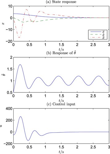
Case A. $\hat{\theta }(0)=-1.0,$ and $x(0)=3.0,\dot{x}(0)=1.0,\ddot{x}(0)=\mathrm{2.0.}$ Case B. $\hat{\theta }(0)=1.5,$ and $x(0)=3.5,\dot{x}(0)=-0.5,\ddot{x}(0)=-1.0.$ The simulation results are shown in Figures 1 and 2. It can be observed that the simulation results are consistent with the theoretical indications. Furthermore, it can be noted that the magnitude of the control u is relatively large, and this is because that the control u has to take the burden to cancel the nonlinearity in the system.

Figure 1. Simulation results for Case A.

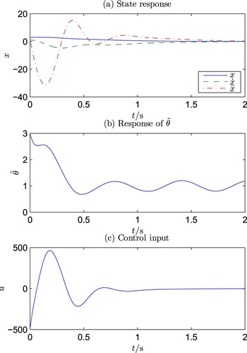
Figure 2. Simulation results for Case B.

8. Conclusion

It has been shown in Parts I (Duan, 2020c) and II (Duan, 2021a) of the series that HOFA models are a type of general system representations and have great advantages in dealing with the control of dynamical systems. As demonstrations, robust control (Duan, 2021b) and adaptive control (Duan, 2021c) of HOFA systems have both been effectively treated. In this paper, the problem of robust adaptive control of a HOFA model is further investigated.

The adaptive control of nonlinear systems with time-varying unknown parameters has always been a difficult problem in the field of systems and control. It is shown that for a HOFA system with nonlinear uncertainties and time-varying unknown parameters, a robust adaptive control law still exists under very mild conditions, which guarantees the global stability (boundedness) of the closed-loop system.

When the unknown parameter vector is constant and the nonlinear uncertainty has a quasi-linear bound, it is further shown that a modified adaptation scheme exists, which does not depend on a pre-estimate of the parameter θ, and guarantees that the state $x^{(0\sim n-1)}$ globally converges to zero while keeping the estimation of the parameter vector bounded.

The proposed approach is very simple and convenient. In the special case that both the nonlinear uncertainties and the unknown parameters do not exist, the closed-loop system reduces to a constant linear system with arbitrarily assignable eigenstructure.

The work of this paper can be extended to the case of sub-fully actuated high-order systems with nonlinear and parametric uncertainties. It can also be extended to different types of systems, such as discrete-time systems and stochastic systems. Furthermore, based on the proposed results, the high-order method of backstepping can also be proposed as treated in Duan (2021b) and Duan (2021c).

Acknowledgements

The author is grateful to his Ph.D. students Guangtai Tian, Qin Zhao, Xiubo Wang, yajun Gao, etc., for helping him with reference selection and proofreading. He is particularly grateful to his student Tianyi Zhao for helping him carrying out the simulation in the example.

Disclosure statement

No potential conflict of interest was reported by the author(s).

Additional information

Funding

This work has been partially supported by the Major Program of National Natural Science Foundation of China [grant numbers 61690210, 61690212], the National Natural Science Foundation of China [grant number 61333003] and the Self-Planned Task of State Key Laboratory of Robotics and System (HIT) [grant number SKLRS201716A].

Notes on contributors

Guangren Duan

Guangren Duan received his Ph.D. degree in Control Systems Sciences from Harbin Institute of Technology, Harbin, P. R. China, in 1989. After a two-year post-doctoral experience at the same university, he became professor of control systems theory at that university in 1991. He is the founder and currently the Director of the Center for Control Theory and Guidance Technology at Harbin Institute of Technology. He visited the University of Hull, the University of Sheffield, and also Queen's University of Belfast, UK, from December 1996 to October 2002, and has served as Member of the Science and Technology committee of the Chinese Ministry of Education, Vice President of the Control Theory and Applications Committee, Chinese Association of Automation (CAA), and Associate Editors of a few international journals. He is currently an Academician of the Chinese Academy of Sciences, and Fellow of CAA, IEEE and IET. His main research interests include parametric control systems design, nonlinear systems, descriptor systems, spacecraft control and magnetic bearing control. He is the author and co-author of 5 books and over 270 SCI indexed publications.

References

- Bartolini, G., Ferrara, A., Giacomini, L., & Usai, E. (1996, December 5–6). A combined backstepping/second order sliding mode approach to control a class of nonlinear systems. Proceedings of International Workshop on Variable Structure Systems, Tokyo, Japan (pp. 205–210). IEEE. https://doi.org/https://doi.org/10.1109/VSS.1996.578620
- Duan, G. R. (1992). Simple algorithm for robust pole assignment in linear output feedback. IEE Proceedings D: Control Theory and Applications, 139(5), 465–470. https://doi.org/https://doi.org/10.1049/ip-d.1992.0058
- Duan, G. R. (1993). Robust eigenstructure assignment via dynamical compensators. Automatica, 29(2), 469–474. https://doi.org/https://doi.org/10.1016/0005-1098(93)90140-O
- Duan, G. R. (2020a). High-order system approaches – I. Full-actuation and parametric design. Acta Automatica Sinica, 46(7), 1333–1345 (in Chinese). https://doi.org/https://doi.org/10.16383/j.aas.c200234
- Duan, G. R. (2020b). High-order system approaches – II. Controllability and fully-actuation. Acta Automatica Sinica, 46(8), 1571–1581 (in Chinese). https://doi.org/https://doi.org/10.16383/j.aas.c200369
- Duan, G. R. (2020c). High-order fully actuated system approaches: I. Models and basic procedure. International Journal of System Sciences, 46(9), 1885–1895. https://doi.org/https://doi.org/10.16383/j.aas.c200370
- Duan, G. R. (2021a). High-order fully actuated system approaches: II. Generalized strict-feedback systems. International Journal of System Sciences. https://doi.org/https://doi.org/10.1080/00207721.2020.1829167
- Duan, G. R. (2021b). High-order fully actuated system approaches: III. Robust control and high-order backstepping. International Journal of System Sciences. https://doi.org/https://doi.org/10.1080/00207721.2020.1829168
- Duan, G. R. (2021c). HOFA system approaches: IV. Adaptive control and high-order backstepping. International Journal of System Sciences. https://doi.org/https://doi.org/10.1080/00207721.2020.1849863
- Duan, G. R. (2021d). HOFA system approaches: VII. Controllability, stabilizability and parametric designs. International Journal of System Sciences. https://doi.org/https://doi.org/10.1080/00207721.2020.1849864
- Duan, G. R., Irwin, G. W., & Liu, G. P. (2002). Disturbance attenuation in linear systems via dynamical compensators: a parametric eigenstructure assignment approach. IEE Proceedings-Control Theory and Applications, 147(2), 129–136. https://doi.org/https://doi.org/10.1049/ip-cta:20000135
- Duan, G. R., Liu, G. P., & Thompson, S. (2000). Disturbance attenuation in Luenberger function observer designs – A parametric approach. IFAC Proceedings Volumes, 33(14), 41–46. https://doi.org/https://doi.org/10.1016/S1474-6670(17)36202-X
- Duan, G. R., & Zhao, T. Y. (2020). Observer-based multi-objective parametric design for spacecraft with super flexible netted antennas. Science China Information Sciences, 63(7), 1–21. Article 172002. https://doi.org/https://doi.org/10.1007/s11432-020-2916-8
- Farrell, J. A., & Polycarpou, M. M. (2006). Adaptive approximation based control: Unifying neural, fuzzy and traditional adaptive approximation approaches. John Wiley and Sons.
- Feuer, A., & Morse, A. S. (1978). Adaptive control of single-input single-output linear systems. IEEE Transactions on Automatic Control, 23(4), 557–569. https://doi.org/https://doi.org/10.1109/TAC.1978.1101822
- Freeman, R. A., Krstić, M., & Kokotović, P. V. (1996). Robustness of adaptive nonlinear control to bounded uncertainties. IFAC Proceedings Volumes, 29(1), 2726–2731. https://doi.org/https://doi.org/10.1016/S1474-6670(17)58088-X
- Gong, J. Q., & Yao, B. (2001). Neural network adaptive robust control of nonlinear systems in semi-strict feedback form. Automatica, 37(8), 1149–1160. https://doi.org/https://doi.org/10.1016/S0005-1098(01)00069-3
- Hou, M. Z., & Duan, G. R. (2011). Robust adaptive dynamic surface control of uncertain nonlinear systems. International Journal of Control, Automation and Systems, 9(1), 161–168. https://doi.org/https://doi.org/10.1007/s12555-011-0121-7
- Jiang, Z. P., & Praly, L. (1991, December 11–13). Iterative designs of adaptive controllers for systems with nonlinear integrators. Proceedings of the 30th IEEE conference on Decision and Control, Brighton, UK (pp. 2482–2487). IEEE. https://doi.org/https://doi.org/10.1109/CDC.1991.261798
- Jiang, Z. P., & Praly, L. (1998). Design of robust adaptive controllers for nonlinear systems with dynamic uncertainties. Automatica, 34(7), 825–840. https://doi.org/https://doi.org/10.1016/S0005-1098(98)00018-1
- Kanellakopoulos, I., Kokotović, P. V., & Morse, A. S. (1991). Systematic design of adaptive controllers for feedback linearizable systems. IEEE Transactions on Automatic Control, 36(11), 1241–1253. https://doi.org/https://doi.org/10.1109/9.100933
- Kokotović, P. V., & Arcak, M. (2001). Constructive nonlinear control: A historical perspective. Automatica, 37(5), 637–662. https://doi.org/https://doi.org/10.1016/S0005-1098(01)00002-4
- Kokotović, P. V., & Kanellakopoulos, I. (1990). Adaptive nonlinear control: A critical appraisal. Proceedings of the sixth Yale Workshop on Adaptive and Learning Systems, New Haven, CT (pp. 1–6). Center for Systems Science, Becton Center, Yale University.
- Kokotović, P. V., Kanellakopoulos, I., & Morse, A. S. (1991). Adaptive feedback linearization of nonlinear systems. In Petar V. Kokotovic (Ed.), Foundations of adaptive control (pp. 309–346), Springer.
- Krstić, M., Kanellakopoulos, I., & Kokotović, P. V. (1992). Adaptive nonlinear control without overparametrization. Systems and Control Letters, 19(3), 177–185. https://doi.org/https://doi.org/10.1016/0167-6911(92)90111-5
- Krstić, M., Kanellakopoulos, I., & Kokotović, P. V. (1995). Nonlinear and adaptive control design. John Wiley and Sons.
- Li, T. S., Wang, D., Feng, G., & Tong, S. C. (2009). A DSC approach to robust adaptive NN tracking control for strict-feedback nonlinear systems. IEEE Transactions on Systems, Man, and Cybernetics-Part B: Cybernetics, 40(3), 915–927. https://doi.org/https://doi.org/10.1109/TSMCB.2009.2033563
- Polycarpou, M. M., & P. A. Ioannou (1996). A robust adaptive nonlinear control design. Automatica, 32(3), 423–427. https://doi.org/https://doi.org/10.1016/0005-1098(95)00147-6
- Rios-Bolívar, M., Zinober, A. S. I., & Sira-Ramírez, H. (1996). Dynamical sliding mode control via adaptive input-output linearization: A backstepping approach. In F. Garofalo and L. Glielmo (Eds.), Robust control via variable structure and Lyapunov techniques (pp. 15–35), Springer-Verlag.
- Tao, G. (2014). Multivariable adaptive control: A survey. Automatica, 50(11), 2737–2764. https://doi.org/https://doi.org/10.1016/j.automatica.2014.10.015
- Yao, B., & Tomizuka, M. (1997). Adaptive robust control of SISO nonlinear systems in a semi-strict feedback form. Automatica, 33(5), 893–900. https://doi.org/https://doi.org/10.1016/S0005-1098(96)00222-1
- Zhu, Y. H., Jiang, C. S., & Fei, S. M. (2003). Robust adaptive dynamic surface control for nonlinear uncertain systems. Joumal of Southeast University, 19(2), 126–131.