High-order fully actuated system approaches: Part VIII. Optimal control with application in spacecraft attitude stabilisation

Abstract

In this paper, the optimal control problem for dynamical systems represented by general high-order fully actuated (HOFA) models is formulated. The problem aims to minimise an objective in the quadratic form of the states and their derivatives of certain orders. The designed controller is a combination of the linearising nonlinear controller and an optimal quadratic controller for a converted linear system. In the infinite-time output regulation case, the solution is in essence a nonlinear state feedback dependent on a well-known Riccati algebraic equation. In the sub-fully actuated system case, the feasibility of the controller is investigated and guaranteed by properly characterising a ball restriction area of the system initial values. Application of the optimal control technique for sub-fully actuated systems to a spacecraft attitude control provides very smooth and steady responses and well demonstrates the effect and simplicity of the proposed approach.

Keywords:

• Optimal control
• fully actuated systems
• output regulation
• feasibility conditions
• attitude control

1. Introduction

Optimal control was born in the late 1950s with the appearance of linear quadratic regulator (LQR), dynamic programming and maximum principle. Kalman (1960) first introduced the LQR for linear systems. The method determines an optimal control in an analytic feedback form and plays a fundamental role in linear control systems theory (Anderson & Moore, 1990). Afterwards, fruitful results appear in the literature. Constrained LQR is proposed for linear systems subject to constraints on the inputs and states (Chmielewski & Manousiouthakis, 1996; Scokaert & Rawlings, 1998), stochastic systems (Chen et al., 1998) and descriptor systems (Bender & Laub, 1987a, 1987b) are also studied, with corresponding LQRs developed, and Terra et al. (2014) considers robust linear quadratic regulators (RLQRs) for discrete-time linear systems with parametric uncertainties, while the noise in state and control is taken into account in Rami et al. (2002). Also, Agrawal (2006) and Li and Chen (2008) extend the optimal control theory to fractional dynamic systems, and the solution to fractional LQR problems is given. In addition, Li and Todorov (2004) present iterative LQR design for nonlinear biological movement systems. In the context of switched and hybrid systems, a number of important properties associated with the discrete-time switched LQR (DSLQR) problem are derived (Zhang et al., 2009, 2012).

Dynamic programming was first proposed by Bellman (1952) with the intension to solve multistage decision process problems. This approach transforms the discrete-time optimal control problem into solving the Hamilton–Jacobi–Bellman (HJB) equation (Bellman & Kalaba, 1957, 1960). For problems involving conflicting objectives, major developments of multi-objective dynamic optimisation have been made, e.g. the fuzzy dynamic programming proposed in Abo-Sinna (2004). To break the ‘curse-of-dimensionality’ associated with the traditional dynamic programming approach, approximate dynamic programming is developed by combining simulation and function approximation (Wang et al., 2009), where heuristic dynamic programming (HDP) (Werbos, 1977), action-dependent HDP (Werbos, 1989), neuro-dynamic programming (Bertsekas & Tsitsiklis, 1995) and learning-based algorithms (Lewis & Vrabie, 2009; Tsitsiklis & Roy, 1997) can be used.

Right around the time Bellman proposed DP, Pontryagin's maximum principle appeared for general continuous-time nonlinear control problem by finding the solution of boundary conditions of the HJB equation (Pontiyagin et al., 1962; Rozonoer, 1959). Later, a discrete version was presented in Hwang and Fan (1967). Nowadays, these types of optimal control techniques have been widely generalised, such as extensions to infinite-dimensional state space (Seierstad, 1975), hybrid control systems with Hybrid Maximum Principle (Dmitruk & Kaganovich, 2008; Sussmann, 1999), constrained impulsive control problems with necessary conditions in the form of Pontryagin's maximum principle (Arutyunov et al., 2012), Boolean control networks (Laschov & Margaliot, 2011a, 2011b) and optimal control problems with time delays (Bokov, 2011).

As a type of optimal control, model predictive control (MPC) techniques provide a methodology to tackle model uncertainty and dynamical constraints on states and inputs without expert intervention (Findeisen et al., 2003; Garcia et al., 1989). The idea originally comes from dynamic matrix control (DMC), and then an explosion of activity in MPC has been witnessed in the current century. For deterministic systems, hybrid MPC, economic MPC, explicit MPC and distributed MPC have attracted much attention. On the other hand, robust MPC and stochastic MPC are proposed to deal with control of uncertain systems subject to disturbances, or state and control constraints. More details can be found in Lee (2011) and Mayne (2014) and the references therein.

Besides the above, H${}_{\mathrm{\infty }}$ optimal control is definitely a celebrated breakthrough, which is developed to deal with the worst-case control design for systems subject to input disturbances (Ball & Helton, 1990; Doyle et al., 1988). The case that parameter uncertainty appears in plant modelling motivates the research on robust H${}_{\mathrm{\infty }}$ control problem, and the results involve both continuous and discrete systems (Xie & de Souza, 1990; Xu et al., 2000). The robust H${}_{\mathrm{\infty }}$ control theory is also extended to time-delay systems (Xu & Chen, 2002). In addition, as an effective approximation method, state-dependent Riccati equation (SDRE)-based methods address nonlinear optimal control problems and provide systematic and effective design of feedback controllers (Çimen, 2008, 2012), where constrained SDRE for systems with state constraints and SDRE in combination with H${}_{\mathrm{\infty }}$, sliding mode control, neural network, etc. are also studied (Nekoo, 2019).

1.1. Fully actuated system approaches

Most the approaches mentioned above are in the general state–space framework. Except those optimal control techniques which are coping with linear systems, e.g. the linear quadratic optimal control, the linear H${}_2$/H${}_{\mathrm{\infty }}$ optimal control, most of the reported optimal control approaches are, more or less, complicated in theory and are hence difficult to apply in practice due to some theoretical or practical obstacles, such as solutions to complicated nonlinear differential or algebraic equations which are not solvable in an accurate sense.

As argued in Duan (2020a), Duan (2020b), Duan (2020d) and Duan (2020j), high-order fully actuated (HOFA) models also serve as a general model for dynamical control systems, and are especially convenient and effective in dealing with control problems. The demonstration of this with robust control, adaptive control and disturbance rejection control has been given in Duan (2020f), Duan (2020g), Duan (2020h) and Duan (2020i). A huge advantage of the HOFA models is that their full-actuation feature allows one to cancel the known nonlinearities in the system and hence to convert, to an extent, a nonlinear problem into a linear one. Such an advantage is again certified in this paper with the problem of nonlinear optimal control.

Any optimal control problem generally has an index, while the most basic form of an index is the quadratic one. In this paper, an optimal control problem for general dynamical systems described by HOFA models is formulated to minimise an index in the quadratic form of the state and its derivatives of certain orders. As a consequence of this requirement, the system responses eventually behave very smoothly and steadily.

As mentioned above, utilising the full-actuation feature of the HOFA models, the nonlinear optimal control problem is converted essentially to a linear quadratic optimal control problem, and a nonlinear optimal controller in a state feedback form is then obtained. Following such an outline, the finite-time optimal tracking control problem is first treated, and then the infinite-time output regulation problem is also solved.

Another contribution of the paper is the treatment of the sub-fully actuated system case. Sub-fully actuated systems are defined in Duan (2020a) and Duan (2020j), and are relatively more difficult to handle due to a problem of feasibility. Using a feature of linear quadratic optimal control, a feasibility condition is established for the optimal control of sub-fully actuated systems. It turns out that feasibility is guaranteed when a condition on only the initial values of the system is met.

For demonstration of the proposed nonlinear optimal control approach, control of the attitude system of a spacecraft is considered. It is well known that the spacecraft attitude system is highly nonlinear when the attitude angles are working in a wide range. Hence accurate attitude manoeuvring with smooth and steady transient performance has ever remained a big challenge. With the new design, stabilisation of the attitude with very smooth and steady transient performance is achieved, and very efficient rapid turning elimination is also realised. The design and simulation results have fully demonstrated that the proposed approach serves a very effective and simple way to tackle such spacecraft attitude control problems.

In the sequential sections, $I_n$ denotes the identity matrix, $\varnothing$ denotes the null set and $\mathrm{\Omega }\mathrm{\setminus }\mathrm{\Theta }$ represents the complement of the set Θ in set Ω. For a square matrix P, ${\lambda }_{max}(P),{\lambda }_{min}(P)$ and $det(P)$ denote its maximum and minimum eigenvalues and its determinant, respectively, while for a nonsingular matrix P, its condition number is denoted by $\nu (P)=\Vert P\Vert \Vert P^{-1}\Vert$. Furthermore, for $x,x_i\in {\mathbb{R}}^m,$ and $A_i\in {\mathbb{R}}^{m\times m},$ $n_0,n_i\in \mathbb{N},n_0<n_i,$ $i=1,2,\dots ,n,$ as in the former papers in the series, $\mathrm{blockdiag}(A_i,i=1,2,\dots ,n)$ denotes a block diagonal matrix with the i-th diagonal block being $A_i,$ and $\begin{array}{rl}& {\Vert x\Vert }_P=x^{\mathrm{T}}Px,\\ & \Vert x\Vert ={\Vert x\Vert }_I=x^{\mathrm{T}}x,\\ & x^{(n_1\sim n_2)}=\left[\begin{array}{c}{x}^{\left(n_1\right)}\\ x^{(n_1+1)}\\ ⋮\\ x^{(n_2)}\end{array}\right],n_1\le n_2,\\ & x_{i\sim j}^{(n_1\sim n_2)}=\left[\begin{array}{c}{x}_i^{(n_1\sim n_2)}\\ x_{i+1}^{(n_1\sim n_2)}\\ ⋮\\ x_j^{(n_1\sim n_2)}\end{array}\right],i\le j,n_1\le n_2,\\ & x_k^{(n_k)}{|}_{k=i\sim j}=\left[\begin{array}{c}{x}_i^{(n_i)}\\ x_{i+1}^{(n_{i+1})}\\ ⋮\\ x_j^{(n_j)}\end{array}\right],i\le j,\\ & x_k^{(n_0\sim n_k)}{|}_{k=i\sim j}=\left[\begin{array}{c}{x}_i^{(n_0\sim n_i)}\\ x_{i+1}^{(n_0\sim n_{i+1})}\\ ⋮\\ x_j^{(n_0\sim n_j)}\end{array}\right],i\le j,\\ & A_{0\sim n-1}=\left[\begin{array}{cccc}{A}_0& A_1& \cdots & A_{n-1}\end{array}\right],\\ & \mathrm{\Phi }(A_{0\sim n-1})=\left[\begin{array}{cccc}0& I& & \\ & & \ddots & \\ & & & I\\ -A_0& -A_1& \cdots & -A_{n-1}\end{array}\right].\end{array}$The paper is organised into seven sections. The next section formulates the nonlinear optimal control problem to be solved in the paper, and a solution to the problem is then given in Section 3. In Sections 4 and 5, the cases of output regulation and sub-fully actuated systems are treated, respectively. An application of the proposed optimal control technique to a spacecraft attitude control problem is presented in Section 6, followed by a brief concluding remark in Section 7. The appendix gives the general attitude model of a spacecraft.

2. Problem formulation

2.1. The HOFA model

Consider the following general HOFA system with multiple orders proposed by Duan (2020j): (1) $\begin{array}{rl}\left[\begin{array}{c}{x}_1^{\left({\mu }_1\right)}\\ x_2^{\left({\mu }_2\right)}\\ ⋮\\ x_{\eta }^{\left({\mu }_{\eta }\right)}\end{array}\right]& =\left[\begin{array}{c}{f}_1(x_k^{(0\sim {\mu }_k-1)}{|}_{k=1\sim \eta },\zeta ,t)\\ f_2(x_k^{(0\sim {\mu }_k-1)}{|}_{k=1\sim \eta },\zeta ,t)\\ ⋮\\ f_{\eta }(x_k^{(0\sim {\mu }_k-1)}{|}_{k=1\sim \eta },\zeta ,t)\end{array}\right]\\ & +B(\cdot )u,\end{array}$(1) where $u\in {\mathbb{R}}^r$ is the control vector, $\zeta \in {\mathbb{R}}^p$ may represent a parameter vector, an external variable vector, a time-delayed state vector, an unmodelled dynamic state vector, etc.; ${\mu }_k,k=1,2,\dots ,\eta ,$ are a set of distinct integers, $x_k\in {\mathbb{R}}^{r_k},k=1,2,\dots ,\eta ,$ are a set of vectors of proper dimensions, with $r_k,k=1,2,\dots ,\eta ,$ being a set of integers satisfying (2) $\begin{array}{r}{r}_1+r_2+\cdots +r_{\eta }=r.\end{array}$(2) Further, $f_k(\cdot )\in {\mathbb{R}}^{r_k},k=1,2,\dots ,\eta ,$ are a set of nonlinear vector functions, and $B(\cdot )=B(x_k^{(0\sim {\mu }_k-1)}{|}_{k=1\sim \eta },\zeta ,t)\in {\mathbb{R}}^{r\times r}$is a sufficiently smooth matrix function satisfying the following full-actuation condition:

Assumption A1

$detB(x_k^{(0\sim {\mu }_k-1)}{|}_{k=1\sim \eta },\zeta ,t)\ne 0,\text{ or}\mathrm{\infty },\text{ for all }{x}_k^{(0\sim {\mu }_k-1)}{|}_{k=1\sim \eta },\zeta$, and t>0.

The system (1(1) $\begin{array}{rl}\left[\begin{array}{c}{x}_1^{\left({\mu }_1\right)}\\ x_2^{\left({\mu }_2\right)}\\ ⋮\\ x_{\eta }^{\left({\mu }_{\eta }\right)}\end{array}\right]& =\left[\begin{array}{c}{f}_1(x_k^{(0\sim {\mu }_k-1)}{|}_{k=1\sim \eta },\zeta ,t)\\ f_2(x_k^{(0\sim {\mu }_k-1)}{|}_{k=1\sim \eta },\zeta ,t)\\ ⋮\\ f_{\eta }(x_k^{(0\sim {\mu }_k-1)}{|}_{k=1\sim \eta },\zeta ,t)\end{array}\right]\\ & +B(\cdot )u,\end{array}$(1) ) satisfying the above Assumption A1 is called a (globally) fully actuated system (Duan, 2020j).

Remark 2.1

The above HOFA model (3(3) $\begin{array}{rl}{x}_k^{\left({\mu }_k\right)}{|}_{k=1\sim \eta }& =f(x_k^{(0\sim {\mu }_k-1)}{|}_{k=1\sim \eta },\zeta ,t)\\ & +B(x_k^{(0\sim {\mu }_k-1)}{|}_{k=1\sim \eta },\zeta ,t)u.\end{array}$(3) ) might be easily mistaken to represent a very small portion of systems due to the full-actuation Assumption A1. While as discussed in Duan (2020a), Duan (2020d) and Duan (2020j), it serves as a general model for dynamical control systems. Many systems which are in state-space forms can be converted into HOFA systems (see Duan (2020a), Duan (2020b), Duan (2020d) and Duan (2020e)), and practical systems can also be modelled as HOFA systems.

If we denote $\begin{array}{rl}& f(x_k^{(0\sim {\mu }_k-1)}{|}_{k=1\sim \eta },\zeta ,t)\\ & =\left[\begin{array}{c}{f}_1(x_k^{(0\sim {\mu }_k-1)}{|}_{k=1\sim \eta },\zeta ,t)\\ f_2(x_k^{(0\sim {\mu }_k-1)}{|}_{k=1\sim \eta },\zeta ,t)\\ ⋮\\ f_{\eta }(x_k^{(0\sim {\mu }_k-1)}{|}_{k=1\sim \eta },\zeta ,t)\end{array}\right],\end{array}$then the HOFA system (1(1) $\begin{array}{rl}\left[\begin{array}{c}{x}_1^{\left({\mu }_1\right)}\\ x_2^{\left({\mu }_2\right)}\\ ⋮\\ x_{\eta }^{\left({\mu }_{\eta }\right)}\end{array}\right]& =\left[\begin{array}{c}{f}_1(x_k^{(0\sim {\mu }_k-1)}{|}_{k=1\sim \eta },\zeta ,t)\\ f_2(x_k^{(0\sim {\mu }_k-1)}{|}_{k=1\sim \eta },\zeta ,t)\\ ⋮\\ f_{\eta }(x_k^{(0\sim {\mu }_k-1)}{|}_{k=1\sim \eta },\zeta ,t)\end{array}\right]\\ & +B(\cdot )u,\end{array}$(1) ) can be compactly written as (3) $\begin{array}{rl}{x}_k^{\left({\mu }_k\right)}{|}_{k=1\sim \eta }& =f(x_k^{(0\sim {\mu }_k-1)}{|}_{k=1\sim \eta },\zeta ,t)\\ & +B(x_k^{(0\sim {\mu }_k-1)}{|}_{k=1\sim \eta },\zeta ,t)u.\end{array}$(3) Recall that $x_k\in {\mathbb{R}}^{r_k}$, $k=1,2,\dots ,\eta ,$ we have $\begin{array}{r}{x}_k^{(0\sim {\mu }_k-1)}\in {\mathbb{R}}^{{\mu }_k{r}_k},k=1,2,\dots ,\eta .\end{array}$Denote (4) $\begin{array}{r}\varkappa =\sum _{k=1}^{\eta }{r}_k{\mu }_k,\end{array}$(4)

then it is easy to see that $\begin{array}{r}{x}_k^{(0\sim {\mu }_k-1)}{|}_{k=1\sim \eta }\in {\mathbb{R}}^{\varkappa }.\end{array}$For the above system (3(3) $\begin{array}{rl}{x}_k^{\left({\mu }_k\right)}{|}_{k=1\sim \eta }& =f(x_k^{(0\sim {\mu }_k-1)}{|}_{k=1\sim \eta },\zeta ,t)\\ & +B(x_k^{(0\sim {\mu }_k-1)}{|}_{k=1\sim \eta },\zeta ,t)u.\end{array}$(3) ), we can impose the output equation (5) $\begin{array}{r}y=C{x}_k^{(0\sim {\mu }_k-1)}{|}_{k=1\sim \eta },\end{array}$(5) where $C\in {\mathbb{R}}^{m\times \varkappa }$ is a known matrix.

Particularly, in the case that the above system (3(3) $\begin{array}{rl}{x}_k^{\left({\mu }_k\right)}{|}_{k=1\sim \eta }& =f(x_k^{(0\sim {\mu }_k-1)}{|}_{k=1\sim \eta },\zeta ,t)\\ & +B(x_k^{(0\sim {\mu }_k-1)}{|}_{k=1\sim \eta },\zeta ,t)u.\end{array}$(3) ) has the following set of output equations (6) $\begin{array}{r}{y}_k=C_k{x}_k^{(0\sim {\mu }_k-1)},k=1,2,\dots ,\eta ,\end{array}$(6) where $C_k,k=1,2,\dots ,\eta ,$ are a set of constant matrices of appropriate dimensions, we can define $\begin{array}{rl}y& =\left[\begin{array}{c}{y}_1\\ y_2\\ ⋮\\ y_{\eta }\end{array}\right],\\ C& =\mathrm{blockdiag}(C_k,k=1,2,\dots ,\eta ),\end{array}$which obeys the output Equation (5(5) $\begin{array}{r}y=C{x}_k^{(0\sim {\mu }_k-1)}{|}_{k=1\sim \eta },\end{array}$(5) ).

2.2. Statement of the problem

The design objective is to let the output y track a properly given sufficiently differentiable signal $z(t)\in {\mathbb{R}}^m$. To realise this, we introduce the following objective: (7) $\begin{array}{rl}{J}_1& =\frac{1}{2}{\int }_0^{t_f}({\Vert y-z\Vert }_Q^2+{\Vert x_k^{\left({\mu }_k\right)}{|}_{k=1\sim \eta }\Vert }_R^2)\mathrm{d}t\\ & +\frac{1}{2}{\Vert y\left(t_f\right)-z\left(t_f\right)\Vert }_S^2,\end{array}$(7) where $Q,S\in {\mathbb{R}}^{m\times m}$ are two semi-positive definite matrices, while $R\in {\mathbb{R}}^{r\times r}$ is a positive definite one. Obviously, the term $\Vert x_k^{({\mu }_k)}{|}_{k=1\sim \eta }{\Vert }_R^2$ in the integral of the above index $J_1$ aims to minimise the changing rate of the system states. As a consequence, smoothness and steadiness in the state vector $x_k^{(0\sim {\mu }_k-1)}{|}_{k=1\sim \eta }$ will be achieved.

Based on the above description, the problem to be solved in this paper can now be stated as follows.

Problem 2.1

Given the HOFA system (3(3) $\begin{array}{rl}{x}_k^{\left({\mu }_k\right)}{|}_{k=1\sim \eta }& =f(x_k^{(0\sim {\mu }_k-1)}{|}_{k=1\sim \eta },\zeta ,t)\\ & +B(x_k^{(0\sim {\mu }_k-1)}{|}_{k=1\sim \eta },\zeta ,t)u.\end{array}$(3) ) with the output Equation (5(5) $\begin{array}{r}y=C{x}_k^{(0\sim {\mu }_k-1)}{|}_{k=1\sim \eta },\end{array}$(5) ), two semi-positive definite matrices $Q,S\in {\mathbb{R}}^{m\times m},$ and a positive definite matrix $R\in {\mathbb{R}}^{r\times r}$, find a feedback controller in the following form: (8) $\begin{array}{rl}u& =-B^{-1}(x_k^{(0\sim {\mu }_k-1)}{|}_{k=1\sim \eta },\zeta ,t)\\ & \times [f(x_k^{(0\sim {\mu }_k-1)}{|}_{k=1\sim \eta },\zeta ,t)-v],\end{array}$(8)

such that the index $J_1$ given by (7(7) $\begin{array}{rl}{J}_1& =\frac{1}{2}{\int }_0^{t_f}({\Vert y-z\Vert }_Q^2+{\Vert x_k^{\left({\mu }_k\right)}{|}_{k=1\sim \eta }\Vert }_R^2)\mathrm{d}t\\ & +\frac{1}{2}{\Vert y\left(t_f\right)-z\left(t_f\right)\Vert }_S^2,\end{array}$(7) ) is minimised, where in (8(8) $\begin{array}{rl}u& =-B^{-1}(x_k^{(0\sim {\mu }_k-1)}{|}_{k=1\sim \eta },\zeta ,t)\\ & \times [f(x_k^{(0\sim {\mu }_k-1)}{|}_{k=1\sim \eta },\zeta ,t)-v],\end{array}$(8) ) (9) $\begin{array}{r}v=v(x_k^{(0\sim {\mu }_k-1)}{|}_{k=1\sim \eta },z,\zeta ,t)\end{array}$(9) is some function which is continuous with respect to its variables.

To end this section, let us finally make some remarks about the considered HOFA model (1(1) $\begin{array}{rl}\left[\begin{array}{c}{x}_1^{\left({\mu }_1\right)}\\ x_2^{\left({\mu }_2\right)}\\ ⋮\\ x_{\eta }^{\left({\mu }_{\eta }\right)}\end{array}\right]& =\left[\begin{array}{c}{f}_1(x_k^{(0\sim {\mu }_k-1)}{|}_{k=1\sim \eta },\zeta ,t)\\ f_2(x_k^{(0\sim {\mu }_k-1)}{|}_{k=1\sim \eta },\zeta ,t)\\ ⋮\\ f_{\eta }(x_k^{(0\sim {\mu }_k-1)}{|}_{k=1\sim \eta },\zeta ,t)\end{array}\right]\\ & +B(\cdot )u,\end{array}$(1) ), or equivalently, (3(3) $\begin{array}{rl}{x}_k^{\left({\mu }_k\right)}{|}_{k=1\sim \eta }& =f(x_k^{(0\sim {\mu }_k-1)}{|}_{k=1\sim \eta },\zeta ,t)\\ & +B(x_k^{(0\sim {\mu }_k-1)}{|}_{k=1\sim \eta },\zeta ,t)u.\end{array}$(3) ).

Remark 2.2

Please note that a special case of the above general HOFA model (1(1) $\begin{array}{rl}\left[\begin{array}{c}{x}_1^{\left({\mu }_1\right)}\\ x_2^{\left({\mu }_2\right)}\\ ⋮\\ x_{\eta }^{\left({\mu }_{\eta }\right)}\end{array}\right]& =\left[\begin{array}{c}{f}_1(x_k^{(0\sim {\mu }_k-1)}{|}_{k=1\sim \eta },\zeta ,t)\\ f_2(x_k^{(0\sim {\mu }_k-1)}{|}_{k=1\sim \eta },\zeta ,t)\\ ⋮\\ f_{\eta }(x_k^{(0\sim {\mu }_k-1)}{|}_{k=1\sim \eta },\zeta ,t)\end{array}\right]\\ & +B(\cdot )u,\end{array}$(1) ) is clearly the following HOFA model with a single-order: (10) $\begin{array}{r}{x}^{\left(n\right)}=f(x^{(0\sim n-1)},\zeta ,t)+B(x^{(0\sim n-1)},\zeta ,t)u,\end{array}$(10) which forms the basic part of the system models involved in the problems of robust control, adaptive control and disturbance rejection treated in Duan (2020f), Duan (2020g), Duan (2020h) and Duan (2020i).

Remark 2.3

Most physical systems are governed by certain physical laws, such as the Newton's Law, the Lagrangian Equation, the Theorem of Linear and Angular Momentum, Kirchhoff's Laws of Current and Voltage. When such physical laws are used in modelling, a series of second-order subsystems are originally obtained (Duan, 2020a). From this stage we can further get a state–space model by variable extension, and on the other side, we can get a HOFA model by variable elimination if the system is controllable (Duan, 2020j). It should be noted that many physically fully actuated systems exist, which are already in the form of second-order HOFA systems at the modelling stage.

3. Solution to problem

The solution to Problem 2.1 can be derived in three steps.

3.1. Step I. Deriving the linear system

In this step, we choose for the system (3(3) $\begin{array}{rl}{x}_k^{\left({\mu }_k\right)}{|}_{k=1\sim \eta }& =f(x_k^{(0\sim {\mu }_k-1)}{|}_{k=1\sim \eta },\zeta ,t)\\ & +B(x_k^{(0\sim {\mu }_k-1)}{|}_{k=1\sim \eta },\zeta ,t)u.\end{array}$(3) ) a control input transformation in the form of (8(8) $\begin{array}{rl}u& =-B^{-1}(x_k^{(0\sim {\mu }_k-1)}{|}_{k=1\sim \eta },\zeta ,t)\\ & \times [f(x_k^{(0\sim {\mu }_k-1)}{|}_{k=1\sim \eta },\zeta ,t)-v],\end{array}$(8) ), with $\begin{array}{r}v=\left[\begin{array}{c}{v}_1\\ v_2\\ ⋮\\ v_{\eta }\end{array}\right]\end{array}$being an introduced control vector. Under this control transformation, the system (3(3) $\begin{array}{rl}{x}_k^{\left({\mu }_k\right)}{|}_{k=1\sim \eta }& =f(x_k^{(0\sim {\mu }_k-1)}{|}_{k=1\sim \eta },\zeta ,t)\\ & +B(x_k^{(0\sim {\mu }_k-1)}{|}_{k=1\sim \eta },\zeta ,t)u.\end{array}$(3) ) is turned into the following series of linear systems: (11) $\begin{array}{r}{x}_k^{\left({\mu }_k\right)}=v_k,k=1,2,\dots ,\eta ,\end{array}$(11) which can be equivalently written in the state-space form as (12) $\begin{array}{rl}{\dot{x}}_k^{(0\sim {\mu }_k-1)}& ={\mathrm{\Phi }}_k{(0_{0\sim {\mu }_k-1})x_k^{(0\sim {\mu }_k-1)}+B}_{kc}{v}_k,\\ k& =1,2,\dots ,\eta ,\end{array}$(12) where, by our notations, (13a) $\begin{array}{rl}{\mathrm{\Phi }}_k\left(0_{0\sim {\mu }_k-1}\right)& =\left[\begin{array}{cccc}0& I_{r_k}& \cdots & 0\\ 0& 0& \ddots & ⋮\\ ⋮& ⋮& \cdots & I_{r_k}\\ 0& 0& \cdots & 0\end{array}\right],\\ B_{kc}& =\left[\begin{array}{c}0\\ ⋮\\ 0\\ I_{r_k}\end{array}\right].\end{array}$(13a) Define $\begin{array}{rl}{A}_E& =\mathrm{blockdiag}({\mathrm{\Phi }}_k\left(0_{0\sim {\mu }_k-1}\right),k=1,2,\dots ,\eta ),\\ B_E& =\mathrm{blockdiag}(B_{kc},k=1,2,\dots ,\eta ),\end{array}$then the set of systems in (12(12) $\begin{array}{rl}{\dot{x}}_k^{(0\sim {\mu }_k-1)}& ={\mathrm{\Phi }}_k{(0_{0\sim {\mu }_k-1})x_k^{(0\sim {\mu }_k-1)}+B}_{kc}{v}_k,\\ k& =1,2,\dots ,\eta ,\end{array}$(12) ) can be more compactly written as (14) $\begin{array}{r}{\dot{x}}_k^{(0\sim {\mu }_k-1)}{|}_{k=1\sim \eta }=A_E{x}_k^{(0\sim {\mu }_k-1)}{|}_{k=1\sim \eta }+B_{E}v.\end{array}$(14)

3.2. Step II. Index conversion

In this step, let us consider the index $J_1$ defined by (7(7) $\begin{array}{rl}{J}_1& =\frac{1}{2}{\int }_0^{t_f}({\Vert y-z\Vert }_Q^2+{\Vert x_k^{\left({\mu }_k\right)}{|}_{k=1\sim \eta }\Vert }_R^2)\mathrm{d}t\\ & +\frac{1}{2}{\Vert y\left(t_f\right)-z\left(t_f\right)\Vert }_S^2,\end{array}$(7) ).

In view of (3(3) $\begin{array}{rl}{x}_k^{\left({\mu }_k\right)}{|}_{k=1\sim \eta }& =f(x_k^{(0\sim {\mu }_k-1)}{|}_{k=1\sim \eta },\zeta ,t)\\ & +B(x_k^{(0\sim {\mu }_k-1)}{|}_{k=1\sim \eta },\zeta ,t)u.\end{array}$(3) ), we have (15) $\begin{array}{rl}{\Vert x_k^{\left({\mu }_k\right)}{|}_{k=1\sim \eta }\Vert }_R^2& =\Vert f(x_k^{(0\sim {\mu }_k-1)}{|}_{k=1\sim \eta },\zeta ,t)\\ & {+B(x_k^{(0\sim {\mu }_k-1)}{|}_{k=1\sim \eta },\zeta ,t)u\Vert }_R^2.\end{array}$(15) Further using (8(8) $\begin{array}{rl}u& =-B^{-1}(x_k^{(0\sim {\mu }_k-1)}{|}_{k=1\sim \eta },\zeta ,t)\\ & \times [f(x_k^{(0\sim {\mu }_k-1)}{|}_{k=1\sim \eta },\zeta ,t)-v],\end{array}$(8) ), we obtain (16) $\begin{array}{rl}v& =f(x_k^{(0\sim {\mu }_k-1)}{|}_{k=1\sim \eta },\zeta ,t)\\ & +B(x_k^{(0\sim {\mu }_k-1)}{|}_{k=1\sim \eta },\zeta ,t)u.\end{array}$(16) Substituting the above relation (16(16) $\begin{array}{rl}v& =f(x_k^{(0\sim {\mu }_k-1)}{|}_{k=1\sim \eta },\zeta ,t)\\ & +B(x_k^{(0\sim {\mu }_k-1)}{|}_{k=1\sim \eta },\zeta ,t)u.\end{array}$(16) ) into (15(15) $\begin{array}{rl}{\Vert x_k^{\left({\mu }_k\right)}{|}_{k=1\sim \eta }\Vert }_R^2& =\Vert f(x_k^{(0\sim {\mu }_k-1)}{|}_{k=1\sim \eta },\zeta ,t)\\ & {+B(x_k^{(0\sim {\mu }_k-1)}{|}_{k=1\sim \eta },\zeta ,t)u\Vert }_R^2.\end{array}$(15) ) gives (17) $\begin{array}{r}{\Vert x_k^{\left({\mu }_k\right)}{|}_{k=1\sim \eta }\Vert }_R^2={\Vert v\Vert }_R^2.\end{array}$(17) Finally, substituting (17(17) $\begin{array}{r}{\Vert x_k^{\left({\mu }_k\right)}{|}_{k=1\sim \eta }\Vert }_R^2={\Vert v\Vert }_R^2.\end{array}$(17) ) into (7(7) $\begin{array}{rl}{J}_1& =\frac{1}{2}{\int }_0^{t_f}({\Vert y-z\Vert }_Q^2+{\Vert x_k^{\left({\mu }_k\right)}{|}_{k=1\sim \eta }\Vert }_R^2)\mathrm{d}t\\ & +\frac{1}{2}{\Vert y\left(t_f\right)-z\left(t_f\right)\Vert }_S^2,\end{array}$(7) ), turns the index $J_1$ into the following form: (18) $\begin{array}{rl}{J}_1& =\frac{1}{2}{\int }_0^{t_f}({\Vert y-z\Vert }_Q^2+{\Vert v\Vert }_R^2)\mathrm{d}t\\ & +\frac{1}{2}{\Vert y\left(t_f\right)-z\left(t_f\right)\Vert }_S^2.\end{array}$(18)

3.3. Step III. Solving the linear optimal problem

In this step, we design a state feedback control law for the linear system (14(14) $\begin{array}{r}{\dot{x}}_k^{(0\sim {\mu }_k-1)}{|}_{k=1\sim \eta }=A_E{x}_k^{(0\sim {\mu }_k-1)}{|}_{k=1\sim \eta }+B_{E}v.\end{array}$(14) ), with the output Equation (5(5) $\begin{array}{r}y=C{x}_k^{(0\sim {\mu }_k-1)}{|}_{k=1\sim \eta },\end{array}$(5) ), to minimise the index $J_1$ defined in (18(18) $\begin{array}{rl}{J}_1& =\frac{1}{2}{\int }_0^{t_f}({\Vert y-z\Vert }_Q^2+{\Vert v\Vert }_R^2)\mathrm{d}t\\ & +\frac{1}{2}{\Vert y\left(t_f\right)-z\left(t_f\right)\Vert }_S^2.\end{array}$(18) ). According to the well-known optimal control result for linear systems (see, e.g. Theorem 8.5.1 in Duan (2016)), the controller is readily obtained as (19) $\begin{array}{r}v=-R^{-1}{B}_E^{\mathrm{T}}P\left(t\right)x_k^{(0\sim {\mu }_k-1)}{|}_{k=1\sim \eta }{+R}^{-1}{B}_E^{\mathrm{T}}g\left(t\right),\end{array}$(19) where $P(t)\in {\mathbb{R}}^{\varkappa \times \varkappa }$ is the solution to the following differential Riccati equation: (20) $\begin{array}{r}-\dot{P}=P{A_E+A}_E^{\mathrm{T}}{P-PB}_E{R}^{-1}{B}_E^{\mathrm{T}}P+C^{\mathrm{T}}QC,\end{array}$(20) with the final value condition (21) $\begin{array}{r}P\left(t_f\right)=C^{\mathrm{T}}SC,\end{array}$(21) and $g(t)\in {\mathbb{R}}^{\varkappa }$ is a vector function satisfying the differential equation (22) $\begin{array}{r}\dot{g}\left(t\right)=A_g\left(t\right)g\left(t\right)-C^{\mathrm{T}}Qz\left(t\right),\end{array}$(22) with (23) $\begin{array}{r}{A}_g\left(t\right)=P\left(t\right)B_E{R}^{-1}{B}_E^{\mathrm{T}}-A_E^{\mathrm{T}},\end{array}$(23) and the final value condition (24) $\begin{array}{r}g\left(t_f\right)=C^{\mathrm{T}}Sz\left(t_f\right).\end{array}$(24) To sum up, we have the following theorem about the solution to Problem 2.1.

Theorem 3.1

Let Assumption A1 be met. Then a solution to Problem 2.1 is given by (25) $\begin{array}{r}\{\begin{array}{l}u=-B^{-1}(x_k^{(0\sim {\mu }_k-1)}{|}_{k=1\sim \eta },\zeta ,t)\\ \times [f(x_k^{(0\sim {\mu }_k-1)}{|}_{k=1\sim \eta },\zeta ,t)-v]\\ v=-R^{-1}{B}_E^{\mathrm{T}}P\left(t\right)x_k^{(0\sim {\mu }_k-1)}{|}_{k=1\sim \eta }{+R}^{-1}{B}_E^{\mathrm{T}}g\left(t\right),\end{array}\end{array}$(25) where $P(t)\in {\mathbb{R}}^{\varkappa \times \varkappa }$ is the solution to the differential Riccati Equation (20(20) $\begin{array}{r}-\dot{P}=P{A_E+A}_E^{\mathrm{T}}{P-PB}_E{R}^{-1}{B}_E^{\mathrm{T}}P+C^{\mathrm{T}}QC,\end{array}$(20) ) subject to the final value condition (21(21) $\begin{array}{r}P\left(t_f\right)=C^{\mathrm{T}}SC,\end{array}$(21) ), and $g(t)\in {\mathbb{R}}^{\varkappa }$ is a vector function satisfying the differential Equations (22(22) $\begin{array}{r}\dot{g}\left(t\right)=A_g\left(t\right)g\left(t\right)-C^{\mathrm{T}}Qz\left(t\right),\end{array}$(22) )–(23(23) $\begin{array}{r}{A}_g\left(t\right)=P\left(t\right)B_E{R}^{-1}{B}_E^{\mathrm{T}}-A_E^{\mathrm{T}},\end{array}$(23) ) and the final value condition (24(24) $\begin{array}{r}g\left(t_f\right)=C^{\mathrm{T}}Sz\left(t_f\right).\end{array}$(24) ).

In the case of output regulation, that is, the case of $z(t)=0$, the index $J_1$ becomes (26) $\begin{array}{rl}{J}_2& =\frac{1}{2}{\int }_0^{t_f}({\Vert y\Vert }_Q^2+{\Vert x_k^{\left({\mu }_k\right)}{|}_{k=1\sim \eta }\Vert }_R^2)\mathrm{d}t\\ & +\frac{1}{2}{\Vert y\left(t_f\right)\Vert }_S^2.\end{array}$(26) In this special case, correspondingly the function $g(t)$ vanishes, and obviously the above Theorem 3.1 becomes the following result.

Corollary 3.1

Let Assumption A1 be met, and $Q,S\in {\mathbb{R}}^{m\times m}$ be semi-positive definite, and $R\in {\mathbb{R}}^{r\times r}$ be positive definite. Then, for the system (3(3) $\begin{array}{rl}{x}_k^{\left({\mu }_k\right)}{|}_{k=1\sim \eta }& =f(x_k^{(0\sim {\mu }_k-1)}{|}_{k=1\sim \eta },\zeta ,t)\\ & +B(x_k^{(0\sim {\mu }_k-1)}{|}_{k=1\sim \eta },\zeta ,t)u.\end{array}$(3) ) with the output Equation (5(5) $\begin{array}{r}y=C{x}_k^{(0\sim {\mu }_k-1)}{|}_{k=1\sim \eta },\end{array}$(5) ), a feedback controller in the form of (8(8) $\begin{array}{rl}u& =-B^{-1}(x_k^{(0\sim {\mu }_k-1)}{|}_{k=1\sim \eta },\zeta ,t)\\ & \times [f(x_k^{(0\sim {\mu }_k-1)}{|}_{k=1\sim \eta },\zeta ,t)-v],\end{array}$(8) ), which minimises the index $J_2,$ is given by (27) $\begin{array}{r}\{\begin{array}{l}u=-B^{-1}(x_k^{(0\sim {\mu }_k-1)}{|}_{k=1\sim \eta },\zeta ,t)\\ \times [f(x_k^{(0\sim {\mu }_k-1)}{|}_{k=1\sim \eta },\zeta ,t)-v]\\ v=-R^{-1}{B}_E^{\mathrm{T}}P\left(t\right)x_k^{(0\sim {\mu }_k-1)}{|}_{k=1\sim \eta }\end{array}\end{array}$(27) where $P(t)\in {\mathbb{R}}^{\varkappa \times \varkappa }$ is the solution to the differential Riccati Equation (20(20) $\begin{array}{r}-\dot{P}=P{A_E+A}_E^{\mathrm{T}}{P-PB}_E{R}^{-1}{B}_E^{\mathrm{T}}P+C^{\mathrm{T}}QC,\end{array}$(20) ) subject to the final value condition (21(21) $\begin{array}{r}P\left(t_f\right)=C^{\mathrm{T}}SC,\end{array}$(21) ).

To end this section, let us make the following remark.

Remark 3.1

In linear systems theory, time-varying linear system context is a very important part. Different from constant linear ones, time-varying linear systems are usually much more difficult to handle. As a matter of fact, the well-known linear quadratic optimal control problem is generally formulated with time-varying linear systems. We point out that, with HOFA approaches, problems related to time-varying linear systems generally do not present since the time-varying terms in the system may be included in the nonlinear term of the HOFA system and hence cancelled by using the full-actuation property.

4. The infinite-time case

4.1. The problem

Let us look into the case of infinite-time output regulation, that is, the case of $z(t)=0$ and $t_f=\mathrm{\infty }.$ Now the final-time term in the objective $J_1$ given in (7(7) $\begin{array}{rl}{J}_1& =\frac{1}{2}{\int }_0^{t_f}({\Vert y-z\Vert }_Q^2+{\Vert x_k^{\left({\mu }_k\right)}{|}_{k=1\sim \eta }\Vert }_R^2)\mathrm{d}t\\ & +\frac{1}{2}{\Vert y\left(t_f\right)-z\left(t_f\right)\Vert }_S^2,\end{array}$(7) ) vanishes, and the objective $J_1$ turns to be (28) $\begin{array}{r}{J}_3=\frac{1}{2}{\int }_0^{\mathrm{\infty }}({\Vert y\Vert }_Q^2+{\Vert x_k^{\left({\mu }_k\right)}{|}_{k=1\sim \eta }\Vert }_R^2)\mathrm{d}t,\end{array}$(28) where $Q\in {\mathbb{R}}^{m\times m}$ is a semi-positive definite matrix, while $R\in {\mathbb{R}}^{r\times r}$ is a positive definite matrix.

Particularly, when the problem of infinite-time state regulation problem is considered, that is, when $C=I_{\varkappa }$ or $y=x_k^{(0\sim {\mu }_k-1)}{|}_{k=1\sim \eta },$ the above index can be simply written as (29) $\begin{array}{rl}{J}_4& =\frac{1}{2}{\int }_0^{\mathrm{\infty }}(x_k^{(0\sim {\mu }_k)}{|}_{k=1\sim \eta }{)}^{\mathrm{T}}\left[\begin{array}{cc}Q& 0\\ 0& R\end{array}\right]\\ & \times x_k^{(0\sim {\mu }_k)}{|}_{k=1\sim \eta }\mathrm{d}t,\end{array}$(29) bearing in mind that the matrix R is required to be symmetric positive definite.

Corresponding to Problem 2.1, now the infinite-time optimal output regulation problem can be stated as follows.

Problem 4.1

Given the HOFA system (3(3) $\begin{array}{rl}{x}_k^{\left({\mu }_k\right)}{|}_{k=1\sim \eta }& =f(x_k^{(0\sim {\mu }_k-1)}{|}_{k=1\sim \eta },\zeta ,t)\\ & +B(x_k^{(0\sim {\mu }_k-1)}{|}_{k=1\sim \eta },\zeta ,t)u.\end{array}$(3) ) with the output Equation (5(5) $\begin{array}{r}y=C{x}_k^{(0\sim {\mu }_k-1)}{|}_{k=1\sim \eta },\end{array}$(5) ), a semi-positive definite matrix $Q\in {\mathbb{R}}^{m\times m}$ and a positive definite matrix $R\in {\mathbb{R}}^{r\times r}$, find for the system a feedback controller in the form of (8(8) $\begin{array}{rl}u& =-B^{-1}(x_k^{(0\sim {\mu }_k-1)}{|}_{k=1\sim \eta },\zeta ,t)\\ & \times [f(x_k^{(0\sim {\mu }_k-1)}{|}_{k=1\sim \eta },\zeta ,t)-v],\end{array}$(8) ), with (30) $\begin{array}{r}v=v(x_k^{(0\sim {\mu }_k-1)}{|}_{k=1\sim \eta },\zeta ,t),\end{array}$(30) such that the index $J_3$ given by (28(28) $\begin{array}{r}{J}_3=\frac{1}{2}{\int }_0^{\mathrm{\infty }}({\Vert y\Vert }_Q^2+{\Vert x_k^{\left({\mu }_k\right)}{|}_{k=1\sim \eta }\Vert }_R^2)\mathrm{d}t,\end{array}$(28) ) is minimised.

Remark 4.1

For the infinite-time optimal control problem, considering tracking an arbitrary signal $z(t)$, as in the finite-time optimal control problem formulated in Section 3, is generally not realisable. However, for certain signal $z(t)$ generated by a proper dynamical system, infinite-time tracking problem can indeed be well formulated and solved (see, e.g. Anderson and Moore (1990)).

4.2. The solution

To derive the solution to the above Problem 4.1, the following well-known result is needed (see, e.g. Lemma 8.3.1 and Theorem 8.3.2 in Duan (2016)).

Lemma 4.2

Let $A\in {\mathbb{R}}^{n\times n}$, $B\in {\mathbb{R}}^{n\times r}$, and $[A,B]$ be controllable. Further let R>0, and $Q=D^{\mathrm{T}}D,$ $[A,D]$ be observable. Then

(1)	the particular solution $P(t)$ to the Riccati differential equation (31) $\begin{array}{r}-\dot{P}=PA+A^{\mathrm{T}}P-PB{R}^{-1}{B}^{\mathrm{T}}P+Q,\end{array}$(31) satisfying the final value condition $P(t_f)=P$ converges uniquely to a constant matrix P, that is, $\begin{array}{r}\underset{t_f\to \mathrm{\infty }}{lim}P\left(t\right)=P;\end{array}$
(2)	this limit matrix P is the unique positive definite solution to the following Riccati algebraic equation $\begin{array}{r}{A}^{\mathrm{T}}P+PA-PB{R}^{-1}{B}^{\mathrm{T}}P+Q=0;\end{array}$
(3)	the following matrix $\begin{array}{r}{A}_c=A-B{R}^{-1}{B}^{\mathrm{T}}P\end{array}$is Hurwitz.

Due to the above lemma, we introduce the following assumption:

Assumption A2

The matrix pair $[A_E,DC]$ is observable, where $D=Q^{\frac{1}{2}}$.

Since $[{\mathrm{\Phi }}_k(0_{0\sim {\mu }_k-1}),B_{kc}],k=1,2,\dots ,\eta$, are all controllable, it is easy to know that $[A_E,B_E]$ is also controllable. Thus it follows from the above Lemma 4.2 and Assumption A1 that the particular solution $P(t)$ to the Riccati differential Equation (20(20) $\begin{array}{r}-\dot{P}=P{A_E+A}_E^{\mathrm{T}}{P-PB}_E{R}^{-1}{B}_E^{\mathrm{T}}P+C^{\mathrm{T}}QC,\end{array}$(20) ) satisfying the final condition $P(t_f)=P$ converges, as $t_f\to \mathrm{\infty }$, to the unique solution of the following Riccati algebraic equation: (32) $\begin{array}{r}{A}_E^{\mathrm{T}}{P+P{A}_E-PB}_E{R}^{-1}{B}_E^{\mathrm{T}}P+C^{\mathrm{T}}QC=0.\end{array}$(32) According to optimal control theory, for the linear system (14(14) $\begin{array}{r}{\dot{x}}_k^{(0\sim {\mu }_k-1)}{|}_{k=1\sim \eta }=A_E{x}_k^{(0\sim {\mu }_k-1)}{|}_{k=1\sim \eta }+B_{E}v.\end{array}$(14) ) the optimal controller which minimise the index (33) $\begin{array}{r}{J}_3^{\mathrm{\prime }}=\frac{1}{2}{\int }_0^{\mathrm{\infty }}({\Vert y\Vert }_Q^2+{\Vert v\Vert }_R^2)\mathrm{d}t\end{array}$(33) is given by $\begin{array}{r}v=-R^{-1}{B}_E^{\mathrm{T}}P{x}_k^{(0\sim {\mu }_k-1)}{|}_{k=1\sim \eta },\end{array}$and the corresponding closed-loop system is (34) $\begin{array}{rl}{\dot{x}}_k^{(0\sim {\mu }_k-1)}{|}_{k=1\sim \eta }& =(A_E-B_E{R}^{-1}{B}_E^{\mathrm{T}}P)\\ & \times x_k^{(0\sim {\mu }_k-1)}{|}_{k=1\sim \eta },\end{array}$(34) which is asymptotically stable according to the above Lemma 4.2.

Based on the above analysis, it is easy to derive the following theorem about the solution to Problem 4.1.

Theorem 4.3

Let Assumptions A1 and A2 be met, and $Q\in {\mathbb{R}}^{m\times m}$ be semi-positive definite, and $R\in {\mathbb{R}}^{r\times r}$ be positive definite. Then, for the system (3(3) $\begin{array}{rl}{x}_k^{\left({\mu }_k\right)}{|}_{k=1\sim \eta }& =f(x_k^{(0\sim {\mu }_k-1)}{|}_{k=1\sim \eta },\zeta ,t)\\ & +B(x_k^{(0\sim {\mu }_k-1)}{|}_{k=1\sim \eta },\zeta ,t)u.\end{array}$(3) ) with the output Equation (5(5) $\begin{array}{r}y=C{x}_k^{(0\sim {\mu }_k-1)}{|}_{k=1\sim \eta },\end{array}$(5) ), a feedback controller in the form of (8(8) $\begin{array}{rl}u& =-B^{-1}(x_k^{(0\sim {\mu }_k-1)}{|}_{k=1\sim \eta },\zeta ,t)\\ & \times [f(x_k^{(0\sim {\mu }_k-1)}{|}_{k=1\sim \eta },\zeta ,t)-v],\end{array}$(8) ), which minimise the index $J_3,$ is given by (35) $\begin{array}{r}\{\begin{array}{l}u=-B^{-1}(x_k^{(0\sim {\mu }_k-1)}{|}_{k=1\sim \eta },\zeta ,t)\\ \times [f(x_k^{(0\sim {\mu }_k-1)}{|}_{k=1\sim \eta },\zeta ,t)-v]\\ v=-R^{-1}{B}_E^{\mathrm{T}}P{x}_k^{(0\sim {\mu }_k-1)}{|}_{k=1\sim \eta }\end{array}\end{array}$(35) where $P\in {\mathbb{R}}^{\varkappa \times \varkappa }$ is the unique solution to the algebraic Riccati Equation (32(32) $\begin{array}{r}{A}_E^{\mathrm{T}}{P+P{A}_E-PB}_E{R}^{-1}{B}_E^{\mathrm{T}}P+C^{\mathrm{T}}QC=0.\end{array}$(32) ). Furthermore, the closed-loop system (34(34) $\begin{array}{rl}{\dot{x}}_k^{(0\sim {\mu }_k-1)}{|}_{k=1\sim \eta }& =(A_E-B_E{R}^{-1}{B}_E^{\mathrm{T}}P)\\ & \times x_k^{(0\sim {\mu }_k-1)}{|}_{k=1\sim \eta },\end{array}$(34) ) is linear and asymptotically stable, and the minimum index is given by (36) $\begin{array}{r}{J}^{\ast }=\frac{1}{2}{\Vert x_k^{(0\sim {\mu }_k-1)}\left(0\right){|}_{k=1\sim \eta }\Vert }_P^2.\end{array}$(36)

Regarding the above result, we make the following remark.

Remark 4.2

Due to the above Theorem 4.3, the optimal controller (35(35) $\begin{array}{r}\{\begin{array}{l}u=-B^{-1}(x_k^{(0\sim {\mu }_k-1)}{|}_{k=1\sim \eta },\zeta ,t)\\ \times [f(x_k^{(0\sim {\mu }_k-1)}{|}_{k=1\sim \eta },\zeta ,t)-v]\\ v=-R^{-1}{B}_E^{\mathrm{T}}P{x}_k^{(0\sim {\mu }_k-1)}{|}_{k=1\sim \eta }\end{array}\end{array}$(35) ) may be viewed as a stabilising controller for the system (3(3) $\begin{array}{rl}{x}_k^{\left({\mu }_k\right)}{|}_{k=1\sim \eta }& =f(x_k^{(0\sim {\mu }_k-1)}{|}_{k=1\sim \eta },\zeta ,t)\\ & +B(x_k^{(0\sim {\mu }_k-1)}{|}_{k=1\sim \eta },\zeta ,t)u.\end{array}$(3) ). However, different from a general stabilising controller for the system, the controller (35(35) $\begin{array}{r}\{\begin{array}{l}u=-B^{-1}(x_k^{(0\sim {\mu }_k-1)}{|}_{k=1\sim \eta },\zeta ,t)\\ \times [f(x_k^{(0\sim {\mu }_k-1)}{|}_{k=1\sim \eta },\zeta ,t)-v]\\ v=-R^{-1}{B}_E^{\mathrm{T}}P{x}_k^{(0\sim {\mu }_k-1)}{|}_{k=1\sim \eta }\end{array}\end{array}$(35) ) also assures that the state vector $x_k^{(0\sim {\mu }_k-1)}(0){|}_{k=1\sim \eta }$ of the closed-loop system goes to zero with a smooth and steady transient performance, and, particularly, $\Vert x_k^{(0\sim {\mu }_k-1)}(t){|}_{k=1\sim \eta }{\Vert }_P$ converges to zero monotonously.

Remark 4.3

Generally speaking, it is hard to achieve global stabilisation (including infinite-time optimal control) of nonlinear systems. However, as demonstrated by the above Theorem 4.3, once a nonlinear system is represented in a HOFA system form, global stabilisation can be easily realised. What is more, the closed-loop system is even linear (which obviously implies global exponential stabilisation). This fact again demonstrates the great advantage of the HOFA design approaches.

5. The sub-fully actuated case

Firstly, let us recall the concept of singular points of sub-fully actuated systems, introduced in Duan (2020j).

5.1. Set of singular points

For a sub-fully actuated system in the form of (1(1) $\begin{array}{rl}\left[\begin{array}{c}{x}_1^{\left({\mu }_1\right)}\\ x_2^{\left({\mu }_2\right)}\\ ⋮\\ x_{\eta }^{\left({\mu }_{\eta }\right)}\end{array}\right]& =\left[\begin{array}{c}{f}_1(x_k^{(0\sim {\mu }_k-1)}{|}_{k=1\sim \eta },\zeta ,t)\\ f_2(x_k^{(0\sim {\mu }_k-1)}{|}_{k=1\sim \eta },\zeta ,t)\\ ⋮\\ f_{\eta }(x_k^{(0\sim {\mu }_k-1)}{|}_{k=1\sim \eta },\zeta ,t)\end{array}\right]\\ & +B(\cdot )u,\end{array}$(1) ), the following concept is essential.

Definition 5.1

If $x_k^{(0\sim {\mu }_k-1)}(t){|}_{k=1\sim \eta }\in {\mathbb{R}}^{\varkappa }$ satisfies (37) $\begin{array}{r}detB(x_k^{(0\sim {\mu }_k-1)}{|}_{k=1\sim \eta },\zeta \left(t\right),t)=0\text{ or }\mathrm{\infty },\end{array}$(37) then it is called a singular point of system (1(1) $\begin{array}{rl}\left[\begin{array}{c}{x}_1^{\left({\mu }_1\right)}\\ x_2^{\left({\mu }_2\right)}\\ ⋮\\ x_{\eta }^{\left({\mu }_{\eta }\right)}\end{array}\right]& =\left[\begin{array}{c}{f}_1(x_k^{(0\sim {\mu }_k-1)}{|}_{k=1\sim \eta },\zeta ,t)\\ f_2(x_k^{(0\sim {\mu }_k-1)}{|}_{k=1\sim \eta },\zeta ,t)\\ ⋮\\ f_{\eta }(x_k^{(0\sim {\mu }_k-1)}{|}_{k=1\sim \eta },\zeta ,t)\end{array}\right]\\ & +B(\cdot )u,\end{array}$(1) ) at time t.

Let ${\mathbb{S}}_t$ be the set of all singular points of system (1(1) $\begin{array}{rl}\left[\begin{array}{c}{x}_1^{\left({\mu }_1\right)}\\ x_2^{\left({\mu }_2\right)}\\ ⋮\\ x_{\eta }^{\left({\mu }_{\eta }\right)}\end{array}\right]& =\left[\begin{array}{c}{f}_1(x_k^{(0\sim {\mu }_k-1)}{|}_{k=1\sim \eta },\zeta ,t)\\ f_2(x_k^{(0\sim {\mu }_k-1)}{|}_{k=1\sim \eta },\zeta ,t)\\ ⋮\\ f_{\eta }(x_k^{(0\sim {\mu }_k-1)}{|}_{k=1\sim \eta },\zeta ,t)\end{array}\right]\\ & +B(\cdot )u,\end{array}$(1) ) at time t, that is, $\begin{array}{r}{\mathbb{S}}_t=\left\{x_k^{(0\sim {\mu }_k-1)}\left(t\right){|}_{k=1\sim \eta }|\text{Equation~(37) holds}\right\}.\end{array}$Then we call, particularly, $\begin{array}{rl}{\mathbb{S}}_0& =\{x_k^{(0\sim {\mu }_k-1)}\left(0\right){|}_{k=1\sim \eta }|\\ & \phantom{x_k^{(0\sim {\mu }_k-1)}}\text{Equation~(37) holds at }t=0\},\end{array}$or, equivalently, $\begin{array}{r}{\mathbb{S}}_0=\{{\mathbb{S}}_t|t=0\},\end{array}$the set of singular initial value points of system (1(1) $\begin{array}{rl}\left[\begin{array}{c}{x}_1^{\left({\mu }_1\right)}\\ x_2^{\left({\mu }_2\right)}\\ ⋮\\ x_{\eta }^{\left({\mu }_{\eta }\right)}\end{array}\right]& =\left[\begin{array}{c}{f}_1(x_k^{(0\sim {\mu }_k-1)}{|}_{k=1\sim \eta },\zeta ,t)\\ f_2(x_k^{(0\sim {\mu }_k-1)}{|}_{k=1\sim \eta },\zeta ,t)\\ ⋮\\ f_{\eta }(x_k^{(0\sim {\mu }_k-1)}{|}_{k=1\sim \eta },\zeta ,t)\end{array}\right]\\ & +B(\cdot )u,\end{array}$(1) ). Furthermore, the following set $\begin{array}{r}\mathbb{S}=\{{\mathbb{S}}_t|t\ge 0\},\end{array}$is called the set of singular points of system (1(1) $\begin{array}{rl}\left[\begin{array}{c}{x}_1^{\left({\mu }_1\right)}\\ x_2^{\left({\mu }_2\right)}\\ ⋮\\ x_{\eta }^{\left({\mu }_{\eta }\right)}\end{array}\right]& =\left[\begin{array}{c}{f}_1(x_k^{(0\sim {\mu }_k-1)}{|}_{k=1\sim \eta },\zeta ,t)\\ f_2(x_k^{(0\sim {\mu }_k-1)}{|}_{k=1\sim \eta },\zeta ,t)\\ ⋮\\ f_{\eta }(x_k^{(0\sim {\mu }_k-1)}{|}_{k=1\sim \eta },\zeta ,t)\end{array}\right]\\ & +B(\cdot )u,\end{array}$(1) ). Clearly, for a HOFA system (1(1) $\begin{array}{rl}\left[\begin{array}{c}{x}_1^{\left({\mu }_1\right)}\\ x_2^{\left({\mu }_2\right)}\\ ⋮\\ x_{\eta }^{\left({\mu }_{\eta }\right)}\end{array}\right]& =\left[\begin{array}{c}{f}_1(x_k^{(0\sim {\mu }_k-1)}{|}_{k=1\sim \eta },\zeta ,t)\\ f_2(x_k^{(0\sim {\mu }_k-1)}{|}_{k=1\sim \eta },\zeta ,t)\\ ⋮\\ f_{\eta }(x_k^{(0\sim {\mu }_k-1)}{|}_{k=1\sim \eta },\zeta ,t)\end{array}\right]\\ & +B(\cdot )u,\end{array}$(1) ) satisfying Assumption A1, there obviously holds $\begin{array}{r}\mathbb{S}={\mathbb{S}}_0={\mathbb{S}}_t=\varnothing ,\mathrm{\forall }t\ge 0.\end{array}$Let us define $\begin{array}{r}\mathbb{F}={\mathbb{R}}^{\varkappa }\mathrm{\setminus }\mathbb{S},\end{array}$then $\mathbb{F}$ is called the set of feasible points of system (1(1) $\begin{array}{rl}\left[\begin{array}{c}{x}_1^{\left({\mu }_1\right)}\\ x_2^{\left({\mu }_2\right)}\\ ⋮\\ x_{\eta }^{\left({\mu }_{\eta }\right)}\end{array}\right]& =\left[\begin{array}{c}{f}_1(x_k^{(0\sim {\mu }_k-1)}{|}_{k=1\sim \eta },\zeta ,t)\\ f_2(x_k^{(0\sim {\mu }_k-1)}{|}_{k=1\sim \eta },\zeta ,t)\\ ⋮\\ f_{\eta }(x_k^{(0\sim {\mu }_k-1)}{|}_{k=1\sim \eta },\zeta ,t)\end{array}\right]\\ & +B(\cdot )u,\end{array}$(1) ). Similarly, the following sets $\begin{array}{r}{\mathbb{F}}_t={\mathbb{R}}^{\varkappa }\mathrm{\setminus }{\mathbb{S}}_t,\end{array}$and $\begin{array}{r}{\mathbb{F}}_0={\mathbb{R}}^{\varkappa }\mathrm{\setminus }{\mathbb{S}}_0,\end{array}$are called the set of feasible points of system (1(1) $\begin{array}{rl}\left[\begin{array}{c}{x}_1^{\left({\mu }_1\right)}\\ x_2^{\left({\mu }_2\right)}\\ ⋮\\ x_{\eta }^{\left({\mu }_{\eta }\right)}\end{array}\right]& =\left[\begin{array}{c}{f}_1(x_k^{(0\sim {\mu }_k-1)}{|}_{k=1\sim \eta },\zeta ,t)\\ f_2(x_k^{(0\sim {\mu }_k-1)}{|}_{k=1\sim \eta },\zeta ,t)\\ ⋮\\ f_{\eta }(x_k^{(0\sim {\mu }_k-1)}{|}_{k=1\sim \eta },\zeta ,t)\end{array}\right]\\ & +B(\cdot )u,\end{array}$(1) ) at time t, and the set of feasible initial value points of system (1(1) $\begin{array}{rl}\left[\begin{array}{c}{x}_1^{\left({\mu }_1\right)}\\ x_2^{\left({\mu }_2\right)}\\ ⋮\\ x_{\eta }^{\left({\mu }_{\eta }\right)}\end{array}\right]& =\left[\begin{array}{c}{f}_1(x_k^{(0\sim {\mu }_k-1)}{|}_{k=1\sim \eta },\zeta ,t)\\ f_2(x_k^{(0\sim {\mu }_k-1)}{|}_{k=1\sim \eta },\zeta ,t)\\ ⋮\\ f_{\eta }(x_k^{(0\sim {\mu }_k-1)}{|}_{k=1\sim \eta },\zeta ,t)\end{array}\right]\\ & +B(\cdot )u,\end{array}$(1) ), respectively. In general, the system (1(1) $\begin{array}{rl}\left[\begin{array}{c}{x}_1^{\left({\mu }_1\right)}\\ x_2^{\left({\mu }_2\right)}\\ ⋮\\ x_{\eta }^{\left({\mu }_{\eta }\right)}\end{array}\right]& =\left[\begin{array}{c}{f}_1(x_k^{(0\sim {\mu }_k-1)}{|}_{k=1\sim \eta },\zeta ,t)\\ f_2(x_k^{(0\sim {\mu }_k-1)}{|}_{k=1\sim \eta },\zeta ,t)\\ ⋮\\ f_{\eta }(x_k^{(0\sim {\mu }_k-1)}{|}_{k=1\sim \eta },\zeta ,t)\end{array}\right]\\ & +B(\cdot )u,\end{array}$(1) ) is called a sub-fully actuated system if $\mathbb{F}$ is a set with dimension not less than 1 (Duan, 2020j).

5.2. Optimal output regulation

With the above preparation, we can now solve the optimal control problem of sub-fully actuated systems. For simplicity, let us again illustrate the idea with the output regulation problem, but with Assumption A1 replaced with the following one.

Assumption A3

The set of singular points, $\mathbb{S},$ meets the following two conditions:

1. it does not depend on time t, that is, $\begin{array}{r}\mathbb{S}={\mathbb{S}}_t={\mathbb{S}}_0,t\ge 0;\end{array}$

2. it does not contain the origin, that is, $\begin{array}{r}{d}_0=inf\{\Vert z\Vert |z\in \mathbb{S}\}>0.\end{array}$

Obviously, the above $d_0$ is clearly the distance of the set $\mathbb{S}$ from the origin. As a consequence of the above Assumption A3, we also have $\begin{array}{r}\mathbb{F}={\mathbb{F}}_0={\mathbb{F}}_t={\mathbb{R}}^{\varkappa }\mathrm{\setminus }\mathbb{S},t\ge 0.\end{array}$With the above preparation, the optimal control problem to be solved can be now stated as follows.

Problem 5.1

Let the HOFA system (3(3) $\begin{array}{rl}{x}_k^{\left({\mu }_k\right)}{|}_{k=1\sim \eta }& =f(x_k^{(0\sim {\mu }_k-1)}{|}_{k=1\sim \eta },\zeta ,t)\\ & +B(x_k^{(0\sim {\mu }_k-1)}{|}_{k=1\sim \eta },\zeta ,t)u.\end{array}$(3) ), with the output Equation (5(5) $\begin{array}{r}y=C{x}_k^{(0\sim {\mu }_k-1)}{|}_{k=1\sim \eta },\end{array}$(5) ), satisfy Assumptions A2 and A3, and $Q\in {\mathbb{R}}^{m\times m}$ be a semi-positive definite matrix, and $R\in {\mathbb{R}}^{r\times r}$ a positive definite one. Find a feedback controller in the form of (8(8) $\begin{array}{rl}u& =-B^{-1}(x_k^{(0\sim {\mu }_k-1)}{|}_{k=1\sim \eta },\zeta ,t)\\ & \times [f(x_k^{(0\sim {\mu }_k-1)}{|}_{k=1\sim \eta },\zeta ,t)-v],\end{array}$(8) ) and (30(30) $\begin{array}{r}v=v(x_k^{(0\sim {\mu }_k-1)}{|}_{k=1\sim \eta },\zeta ,t),\end{array}$(30) ), such that

(1)	the index $J_3$ given by (28(28) $\begin{array}{r}{J}_3=\frac{1}{2}{\int }_0^{\mathrm{\infty }}({\Vert y\Vert }_Q^2+{\Vert x_k^{\left({\mu }_k\right)}{|}_{k=1\sim \eta }\Vert }_R^2)\mathrm{d}t,\end{array}$(28) ) is minimised and
(2)	the following feasibility condition is met: (38) $\begin{array}{r}{x}_k^{(0\sim {\mu }_k-1)}{|}_{k=1\sim \eta }\in \mathbb{F}.\end{array}$(38)

To solve the above problem, we need to present the following important lemma about stabilisation of sub-fully actuated systems.

Lemma 5.2

Let Assumption A3 be met. Further, let $K\in {\mathbb{R}}^{r\times \varkappa }$ be a matrix making $\begin{array}{r}{A}_c=A_E+B_{E}K\end{array}$Hurwitz, and $P\in {\mathbb{R}}^{\varkappa \times \varkappa }$ be a positive definite matrix satisfying the Lyapunov matrix equation $\begin{array}{r}{A}_c^{\mathrm{T}}{P}_c+P_c{A}_c+D_c^{\mathrm{T}}{D}_c=0,\end{array}$where $D_c\in {\mathbb{R}}^{q\times \varkappa },$ $q\le \varkappa ,$ and $[A,D_c]$ is observable. Then,

(1)

the following feedback controller (39) $\begin{array}{r}\{\begin{array}{l}u=-B^{-1}(x_k^{(0\sim {\mu }_k-1)}{|}_{k=1\sim \eta },\zeta ,t)\\ \times [f(x_k^{(0\sim {\mu }_k-1)}{|}_{k=1\sim \eta },\zeta ,t)-v]\\ v=K{x}_k^{(0\sim {\mu }_k-1)}{|}_{k=1\sim \eta }\end{array}\end{array}$(39) stabilises the HOFA system (3(3) $\begin{array}{rl}{x}_k^{\left({\mu }_k\right)}{|}_{k=1\sim \eta }& =f(x_k^{(0\sim {\mu }_k-1)}{|}_{k=1\sim \eta },\zeta ,t)\\ & +B(x_k^{(0\sim {\mu }_k-1)}{|}_{k=1\sim \eta },\zeta ,t)u.\end{array}$(3) ) and

(2)

if, further, the initial values are chosen to satisfy (40) $\begin{array}{r}\sqrt{\nu \left(P_c\right)}\Vert x_k^{(0\sim {\mu }_k-1)}\left(0\right){|}_{k=1\sim \eta }\Vert <d_0,\end{array}$(40) then the feasibility condition (38(38) $\begin{array}{r}{x}_k^{(0\sim {\mu }_k-1)}{|}_{k=1\sim \eta }\in \mathbb{F}.\end{array}$(38) ) is also met.

Proof.

Under given conditions, the first conclusion can be easily proven, now we need only to show that the feasibility requirement (38(38) $\begin{array}{r}{x}_k^{(0\sim {\mu }_k-1)}{|}_{k=1\sim \eta }\in \mathbb{F}.\end{array}$(38) ) is met when condition (40(40) $\begin{array}{r}\sqrt{\nu \left(P_c\right)}\Vert x_k^{(0\sim {\mu }_k-1)}\left(0\right){|}_{k=1\sim \eta }\Vert <d_0,\end{array}$(40) ) holds.

First of all, since $\nu (P_c)\ge 1,$ it follows from (40(40) $\begin{array}{r}\sqrt{\nu \left(P_c\right)}\Vert x_k^{(0\sim {\mu }_k-1)}\left(0\right){|}_{k=1\sim \eta }\Vert <d_0,\end{array}$(40) ) that (41) $\begin{array}{r}\Vert x_k^{(0\sim {\mu }_k-1)}\left(0\right){|}_{k=1\sim \eta }\Vert <\frac{1}{\sqrt{\nu \left(P_c\right)}}{d}_0\le d_0.\end{array}$(41) Thus we have (42) $\begin{array}{r}{x}_k^{(0\sim {\mu }_k-1)}{|}_{k=1\sim \eta }\left(0\right)\in \mathbb{F}.\end{array}$(42) Next, let us define $\begin{array}{r}V\left(t\right)={\Vert x_k^{(0\sim {\mu }_k-1)}\left(t\right){|}_{k=1\sim \eta }\Vert }_{P_c}^2,\end{array}$then, following a typical treatment in stability analysis of linear systems, we can prove that $\begin{array}{r}\dot{V}\left(t\right)\le 0.\end{array}$Therefore, $\begin{array}{r}V\left(t\right)\le V\left(0\right),\mathrm{\forall }t\ge 0,\end{array}$that is, (43) $\begin{array}{rl}& {\Vert x_k^{(0\sim {\mu }_k-1)}\left(t\right){|}_{k=1\sim \eta }\Vert }_{P_c}^2\\ & \le {\Vert x_k^{(0\sim {\mu }_k-1)}\left(0\right){|}_{k=1\sim \eta }\Vert }_{P_c}^2,\mathrm{\forall }t\ge 0.\end{array}$(43) From this we obtain, for $t\ge 0$, $\begin{array}{rl}& {\lambda }_{min}\left(P_c\right){\Vert x_k^{(0\sim {\mu }_k-1)}\left(t\right){|}_{k=1\sim \eta }\Vert }^2\\ & \le {\lambda }_{max}\left(P_c\right){\Vert x_k^{(0\sim {\mu }_k-1)}\left(0\right){|}_{k=1\sim \eta }\Vert }^2,\end{array}$which further gives, together with condition (40(40) $\begin{array}{r}\sqrt{\nu \left(P_c\right)}\Vert x_k^{(0\sim {\mu }_k-1)}\left(0\right){|}_{k=1\sim \eta }\Vert <d_0,\end{array}$(40) ), the following $\begin{array}{rl}& {\Vert x_k^{(0\sim {\mu }_k-1)}\left(t\right){|}_{k=1\sim \eta }\Vert }^2\\ & \le \frac{{\lambda }_{max}\left(P_c\right)}{{\lambda }_{min}\left(P_c\right)}{\Vert x_k^{(0\sim {\mu }_k-1)}\left(0\right){|}_{k=1\sim \eta }\Vert }^2\\ & =\Vert P_c\Vert \Vert P_c^{-1}\Vert {\Vert x_k^{(0\sim {\mu }_k-1)}\left(0\right){|}_{k=1\sim \eta }\Vert }^2\\ & =\nu \left(P_c\right){\Vert x_k^{(0\sim {\mu }_k-1)}\left(0\right){|}_{k=1\sim \eta }\Vert }^2\\ & \le d_0^2.\end{array}$This implies the relation (38(38) $\begin{array}{r}{x}_k^{(0\sim {\mu }_k-1)}{|}_{k=1\sim \eta }\in \mathbb{F}.\end{array}$(38) ). The proof is then completed.

Based on Theorem 4.3 and the above lemma, a solution to the above Problem 5.1 can be given as follows.

Theorem 5.3

Let Assumptions A2 and A3 be met, and $Q\in {\mathbb{R}}^{m\times m}$ be semi-positive definite, and $R\in {\mathbb{R}}^{r\times r}$ be positive definite. Further, let the feedback controller in the form of (8(8) $\begin{array}{rl}u& =-B^{-1}(x_k^{(0\sim {\mu }_k-1)}{|}_{k=1\sim \eta },\zeta ,t)\\ & \times [f(x_k^{(0\sim {\mu }_k-1)}{|}_{k=1\sim \eta },\zeta ,t)-v],\end{array}$(8) ) for the system (3(3) $\begin{array}{rl}{x}_k^{\left({\mu }_k\right)}{|}_{k=1\sim \eta }& =f(x_k^{(0\sim {\mu }_k-1)}{|}_{k=1\sim \eta },\zeta ,t)\\ & +B(x_k^{(0\sim {\mu }_k-1)}{|}_{k=1\sim \eta },\zeta ,t)u.\end{array}$(3) ) be given by (35(35) $\begin{array}{r}\{\begin{array}{l}u=-B^{-1}(x_k^{(0\sim {\mu }_k-1)}{|}_{k=1\sim \eta },\zeta ,t)\\ \times [f(x_k^{(0\sim {\mu }_k-1)}{|}_{k=1\sim \eta },\zeta ,t)-v]\\ v=-R^{-1}{B}_E^{\mathrm{T}}P{x}_k^{(0\sim {\mu }_k-1)}{|}_{k=1\sim \eta }\end{array}\end{array}$(35) ), with $P\in {\mathbb{R}}^{\varkappa \times \varkappa }$ being the unique solution to the algebraic Riccati Equation (32(32) $\begin{array}{r}{A}_E^{\mathrm{T}}{P+P{A}_E-PB}_E{R}^{-1}{B}_E^{\mathrm{T}}P+C^{\mathrm{T}}QC=0.\end{array}$(32) ). If, further, the initial values are chosen to satisfy (44) $\begin{array}{r}\sqrt{\nu \left(P\right)}\Vert x_k^{(0\sim {\mu }_k-1)}\left(0\right){|}_{k=1\sim \eta }\Vert <d_0,\end{array}$(44) then the two requirements in Problem 5.1 are both met.

Proof.

Denote (45) $\begin{array}{rl}K& =-R^{-1}{B}_E^{\mathrm{T}}P,\end{array}$(45) (46) $\begin{array}{rl}{A}_c& =A_E+B_{E}K,\end{array}$(46) then, by Theorem 4.3, $A_c$ is Hurwitz. Further note $\begin{array}{r}{A}_c^{\mathrm{T}}{P+P{A}_c=A}_E^{\mathrm{T}}{P+P{A}_E-2PB}_E{R}^{-1}{B}_E^{\mathrm{T}}P,\end{array}$it is clear that the Riccati Equation (32(32) $\begin{array}{r}{A}_E^{\mathrm{T}}{P+P{A}_E-PB}_E{R}^{-1}{B}_E^{\mathrm{T}}P+C^{\mathrm{T}}QC=0.\end{array}$(32) ) is equivalent to the following Lyapunov matrix equation (47) $\begin{array}{r}{A}_c^{\mathrm{T}}P+P{A}_c+Q_c=0,\end{array}$(47) with (48) $\begin{array}{r}{Q}_c=C^{\mathrm{T}}QC+{PB}_E{R}^{-1}{B}_E^{\mathrm{T}}P.\end{array}$(48) Due to Assumption A2, we have $Q=D^{\mathrm{T}}D,$ and $[A_E,DC]$ is observable. Further let $\begin{array}{r}{R}^{-1}=T{T}^{\mathrm{T}},\end{array}$we can write (49) $\begin{array}{rl}{Q}_c& ={\left(DC\right)}^{\mathrm{T}}DC+{PB}_{E}T{T}^{\mathrm{T}}{B}_E^{\mathrm{T}}P\\ & =\left[{\left(DC\right)}^{\mathrm{T}}{PB}_{E}T\right]\left[\begin{array}{c}DC\\ {\left({PB}_{E}T\right)}^{\mathrm{T}}\end{array}\right].\end{array}$(49) Remembering that $[A_E,DC]$ is observable, by the well-known PBH criterion we have $\begin{array}{r}\mathrm{rank}\left[\begin{array}{c}sI-A_E\\ DC\end{array}\right]=\varkappa ,\mathrm{\forall }s\in \mathbb{C}.\end{array}$Using this relation, we immediately have (50) $\begin{array}{r}\mathrm{rank}\left[\begin{array}{c}sI-A_E\\ DC\\ {\left({PB}_{E}T\right)}^{\mathrm{T}}\end{array}\right]=\varkappa ,\mathrm{\forall }s\in \mathbb{C},\end{array}$(50) that is, the matrix pair $\begin{array}{r}[A_E,\left[\begin{array}{c}DC\\ {\left({PB}_{E}T\right)}^{\mathrm{T}}\end{array}\right]]\end{array}$is also observable by the PBH criterion again. Therefore, the conclusion of the theorem can now be easily drawn by combining Theorem 4.3 and Lemma 5.2.

5.3. Further discussions

This section further looks into two circumstances.

5.3.1. Case of $\mathbb{S}$ containing the origin

For simplicity, let us consider the following time-invariant HOFA system: (51) $\begin{array}{rl}\left[\begin{array}{c}{x}_1^{\left({\mu }_1\right)}\\ x_2^{\left({\mu }_2\right)}\\ ⋮\\ x_{\eta }^{\left({\mu }_{\eta }\right)}\end{array}\right]& =\left[\begin{array}{c}{f}_1\left(x_k^{(0\sim {\mu }_k-1)}{|}_{k=1\sim \eta }\right)\\ f_2\left(x_k^{(0\sim {\mu }_k-1)}{|}_{k=1\sim \eta }\right)\\ ⋮\\ f_{\eta }\left(x_k^{(0\sim {\mu }_k-1)}{|}_{k=1\sim \eta }\right)\end{array}\right]\\ & +B\left(x_k^{(0\sim {\mu }_k-1)}{|}_{k=1\sim \eta }\right)u.\end{array}$(51) By definition, its set of singular points is $\begin{array}{rl}{\mathbb{S}}^x& =\{x_k^{(0\sim {\mu }_k-1)}{|}_{k=1\sim \eta }|\\ & detB\left(x_k^{(0\sim {\mu }_k-1)}{|}_{k=1\sim \eta }\right)=0\text{ or }\mathrm{\infty }\}.\end{array}$When the above set of singular points contains the origin, we can introduce a state transformation (52) $\begin{array}{r}{z}_k^{(0\sim {\mu }_k-1)}{|}_{k=1\sim \eta }=x_k^{(0\sim {\mu }_k-1)}{|}_{k=1\sim \eta }-q,\end{array}$(52) where $q\in {\mathbb{R}}^{\varkappa }$ is a constant vector. Under the above transformation, the above system (51(51) $\begin{array}{rl}\left[\begin{array}{c}{x}_1^{\left({\mu }_1\right)}\\ x_2^{\left({\mu }_2\right)}\\ ⋮\\ x_{\eta }^{\left({\mu }_{\eta }\right)}\end{array}\right]& =\left[\begin{array}{c}{f}_1\left(x_k^{(0\sim {\mu }_k-1)}{|}_{k=1\sim \eta }\right)\\ f_2\left(x_k^{(0\sim {\mu }_k-1)}{|}_{k=1\sim \eta }\right)\\ ⋮\\ f_{\eta }\left(x_k^{(0\sim {\mu }_k-1)}{|}_{k=1\sim \eta }\right)\end{array}\right]\\ & +B\left(x_k^{(0\sim {\mu }_k-1)}{|}_{k=1\sim \eta }\right)u.\end{array}$(51) ) is converted into (53) $\begin{array}{rl}\left[\begin{array}{c}{z}_1^{\left({\mu }_1\right)}\\ z_2^{\left({\mu }_2\right)}\\ ⋮\\ z_{\eta }^{\left({\mu }_{\eta }\right)}\end{array}\right]& =\left[\begin{array}{c}{f}_1(z_k^{(0\sim {\mu }_k-1)}{|}_{k=1\sim \eta },q)\\ f_2(z_k^{(0\sim {\mu }_k-1)}{|}_{k=1\sim \eta },q)\\ ⋮\\ f_{\eta }(z_k^{(0\sim {\mu }_k-1)}{|}_{k=1\sim \eta },q)\end{array}\right]\\ & +B(z_k^{(0\sim {\mu }_k-1)}{|}_{k=1\sim \eta },q)u.\end{array}$(53) Often with a proper choice of the constant vector q, the set of singular points of the above new system (53(53) $\begin{array}{rl}\left[\begin{array}{c}{z}_1^{\left({\mu }_1\right)}\\ z_2^{\left({\mu }_2\right)}\\ ⋮\\ z_{\eta }^{\left({\mu }_{\eta }\right)}\end{array}\right]& =\left[\begin{array}{c}{f}_1(z_k^{(0\sim {\mu }_k-1)}{|}_{k=1\sim \eta },q)\\ f_2(z_k^{(0\sim {\mu }_k-1)}{|}_{k=1\sim \eta },q)\\ ⋮\\ f_{\eta }(z_k^{(0\sim {\mu }_k-1)}{|}_{k=1\sim \eta },q)\end{array}\right]\\ & +B(z_k^{(0\sim {\mu }_k-1)}{|}_{k=1\sim \eta },q)u.\end{array}$(53) ), namely, ${\mathbb{S}}^z,$ does not contain the origin. Hence for the system (53(53) $\begin{array}{rl}\left[\begin{array}{c}{z}_1^{\left({\mu }_1\right)}\\ z_2^{\left({\mu }_2\right)}\\ ⋮\\ z_{\eta }^{\left({\mu }_{\eta }\right)}\end{array}\right]& =\left[\begin{array}{c}{f}_1(z_k^{(0\sim {\mu }_k-1)}{|}_{k=1\sim \eta },q)\\ f_2(z_k^{(0\sim {\mu }_k-1)}{|}_{k=1\sim \eta },q)\\ ⋮\\ f_{\eta }(z_k^{(0\sim {\mu }_k-1)}{|}_{k=1\sim \eta },q)\end{array}\right]\\ & +B(z_k^{(0\sim {\mu }_k-1)}{|}_{k=1\sim \eta },q)u.\end{array}$(53) ) Assumption A3 holds. Therefore, the optimal control of system (51(51) $\begin{array}{rl}\left[\begin{array}{c}{x}_1^{\left({\mu }_1\right)}\\ x_2^{\left({\mu }_2\right)}\\ ⋮\\ x_{\eta }^{\left({\mu }_{\eta }\right)}\end{array}\right]& =\left[\begin{array}{c}{f}_1\left(x_k^{(0\sim {\mu }_k-1)}{|}_{k=1\sim \eta }\right)\\ f_2\left(x_k^{(0\sim {\mu }_k-1)}{|}_{k=1\sim \eta }\right)\\ ⋮\\ f_{\eta }\left(x_k^{(0\sim {\mu }_k-1)}{|}_{k=1\sim \eta }\right)\end{array}\right]\\ & +B\left(x_k^{(0\sim {\mu }_k-1)}{|}_{k=1\sim \eta }\right)u.\end{array}$(51) ) can then be solved by applying the above Theorem 5.3 to the transformed system (53(53) $\begin{array}{rl}\left[\begin{array}{c}{z}_1^{\left({\mu }_1\right)}\\ z_2^{\left({\mu }_2\right)}\\ ⋮\\ z_{\eta }^{\left({\mu }_{\eta }\right)}\end{array}\right]& =\left[\begin{array}{c}{f}_1(z_k^{(0\sim {\mu }_k-1)}{|}_{k=1\sim \eta },q)\\ f_2(z_k^{(0\sim {\mu }_k-1)}{|}_{k=1\sim \eta },q)\\ ⋮\\ f_{\eta }(z_k^{(0\sim {\mu }_k-1)}{|}_{k=1\sim \eta },q)\end{array}\right]\\ & +B(z_k^{(0\sim {\mu }_k-1)}{|}_{k=1\sim \eta },q)u.\end{array}$(53) ).

5.3.2. Decoupled designs

It is easily recognised from the proof of Theorem 5.3 that the subset of the feasible initial values given by Theorem 5.3, that is, the set of points satisfying condition (44(44) $\begin{array}{r}\sqrt{\nu \left(P\right)}\Vert x_k^{(0\sim {\mu }_k-1)}\left(0\right){|}_{k=1\sim \eta }\Vert <d_0,\end{array}$(44) ), may be conservative. In certain cases, e.g. when $detB(x_k^{(0\sim {\mu }_k-1)}{|}_{k=1\sim \eta })$ is dependent on only some, but not all, $x_k$'s and their derivatives, less conservative initial value ranges can be provided.

For convenience, let us simply assume that $detB(x_k^{(0\sim {\mu }_k-1)}{|}_{k=1\sim \eta })$ is dependent on only $x_{\eta }^{(0\sim {\mu }_{\eta }-1)},$ that is, there exists a scalar function $h(x_{\eta }^{(0\sim {\mu }_{\eta }-1)})$ such that $\begin{array}{r}detB\left(x_k^{(0\sim {\mu }_k-1)}{|}_{k=1\sim \eta }\right)=h\left(x_{\eta }^{(0\sim {\mu }_{\eta }-1)}\right).\end{array}$In this case, instead of converting (51(51) $\begin{array}{rl}\left[\begin{array}{c}{x}_1^{\left({\mu }_1\right)}\\ x_2^{\left({\mu }_2\right)}\\ ⋮\\ x_{\eta }^{\left({\mu }_{\eta }\right)}\end{array}\right]& =\left[\begin{array}{c}{f}_1\left(x_k^{(0\sim {\mu }_k-1)}{|}_{k=1\sim \eta }\right)\\ f_2\left(x_k^{(0\sim {\mu }_k-1)}{|}_{k=1\sim \eta }\right)\\ ⋮\\ f_{\eta }\left(x_k^{(0\sim {\mu }_k-1)}{|}_{k=1\sim \eta }\right)\end{array}\right]\\ & +B\left(x_k^{(0\sim {\mu }_k-1)}{|}_{k=1\sim \eta }\right)u.\end{array}$(51) ) into a whole system (14(14) $\begin{array}{r}{\dot{x}}_k^{(0\sim {\mu }_k-1)}{|}_{k=1\sim \eta }=A_E{x}_k^{(0\sim {\mu }_k-1)}{|}_{k=1\sim \eta }+B_{E}v.\end{array}$(14) ), we can convert (51(51) $\begin{array}{rl}\left[\begin{array}{c}{x}_1^{\left({\mu }_1\right)}\\ x_2^{\left({\mu }_2\right)}\\ ⋮\\ x_{\eta }^{\left({\mu }_{\eta }\right)}\end{array}\right]& =\left[\begin{array}{c}{f}_1\left(x_k^{(0\sim {\mu }_k-1)}{|}_{k=1\sim \eta }\right)\\ f_2\left(x_k^{(0\sim {\mu }_k-1)}{|}_{k=1\sim \eta }\right)\\ ⋮\\ f_{\eta }\left(x_k^{(0\sim {\mu }_k-1)}{|}_{k=1\sim \eta }\right)\end{array}\right]\\ & +B\left(x_k^{(0\sim {\mu }_k-1)}{|}_{k=1\sim \eta }\right)u.\end{array}$(51) ) into two subsystems in state–space forms, as (54) $\begin{array}{r}{\dot{x}}_{\eta }^{(0\sim {\mu }_{\eta }-1)}={\mathrm{\Phi }}_{\eta }{(0_{0\sim {\mu }_{\eta }-1})x_{\eta }^{(0\sim {\mu }_{\eta }-1)}+B}_{\eta c}{v}_{\eta },\end{array}$(54) and (55) $\begin{array}{rl}& {\dot{x}}_k^{(0\sim {\mu }_k-1)}{|}_{k=1\sim \eta -1}\\ & =A_E^{\mathrm{\prime }}{x}_k^{(0\sim {\mu }_k-1)}{|}_{k=1\sim \eta -1}+B_E^{\mathrm{\prime }}{v}_{1\sim \eta -1},\end{array}$(55) where $\begin{array}{rl}& v_{1\sim \eta -1}=\left[\begin{array}{c}{v}_1\\ v_2\\ ⋮\\ v_{\eta -1}\end{array}\right],\\ & A_E^{\mathrm{\prime }}=\mathrm{blockdiag}({\mathrm{\Phi }}_k\left(0_{0\sim {\mu }_k-1}\right),k=1,2,\dots ,\eta -1),\\ & B_E^{\mathrm{\prime }}=\mathrm{blockdiag}(B_{kc},k=1,2,\dots ,\eta -1).\end{array}$By now, in the Step III of Section 3, we can apply the linear quadratic regulation control technique to both systems (54(54) $\begin{array}{r}{\dot{x}}_{\eta }^{(0\sim {\mu }_{\eta }-1)}={\mathrm{\Phi }}_{\eta }{(0_{0\sim {\mu }_{\eta }-1})x_{\eta }^{(0\sim {\mu }_{\eta }-1)}+B}_{\eta c}{v}_{\eta },\end{array}$(54) ) and (55(55) $\begin{array}{rl}& {\dot{x}}_k^{(0\sim {\mu }_k-1)}{|}_{k=1\sim \eta -1}\\ & =A_E^{\mathrm{\prime }}{x}_k^{(0\sim {\mu }_k-1)}{|}_{k=1\sim \eta -1}+B_E^{\mathrm{\prime }}{v}_{1\sim \eta -1},\end{array}$(55) ) separately, as treated in the proof of Theorem 3.1. As a consequence, the initial values of the system (55(55) $\begin{array}{rl}& {\dot{x}}_k^{(0\sim {\mu }_k-1)}{|}_{k=1\sim \eta -1}\\ & =A_E^{\mathrm{\prime }}{x}_k^{(0\sim {\mu }_k-1)}{|}_{k=1\sim \eta -1}+B_E^{\mathrm{\prime }}{v}_{1\sim \eta -1},\end{array}$(55) ) can be freely chosen, while only the initial values of the system (54(54) $\begin{array}{r}{\dot{x}}_{\eta }^{(0\sim {\mu }_{\eta }-1)}={\mathrm{\Phi }}_{\eta }{(0_{0\sim {\mu }_{\eta }-1})x_{\eta }^{(0\sim {\mu }_{\eta }-1)}+B}_{\eta c}{v}_{\eta },\end{array}$(54) ) should be properly restricted to meet the feasibility of the controller (8(8) $\begin{array}{rl}u& =-B^{-1}(x_k^{(0\sim {\mu }_k-1)}{|}_{k=1\sim \eta },\zeta ,t)\\ & \times [f(x_k^{(0\sim {\mu }_k-1)}{|}_{k=1\sim \eta },\zeta ,t)-v],\end{array}$(8) ), as treated in the proof of the above Theorem 5.3. In such a way, a much more tight subset of feasible initial values can be provided. The next section gives a demonstration of this idea with an application to spacecraft attitude control.

6. Spacecraft attitude control

6.1. The system model

Consider the modelling of the attitude system of a spacecraft. The coordinate system on the spacecraft is shown in Figure 1. The origin of the coordinate system is taken to be the centre of the spacecraft, the z-axis takes the direction from the centre of the spacecraft to the earth centre, the x-axis goes along with the flight direction of the spacecraft, and the y-axis is determined by the right-hand coordinate system.

Figure 1. Coordinate system transformation.

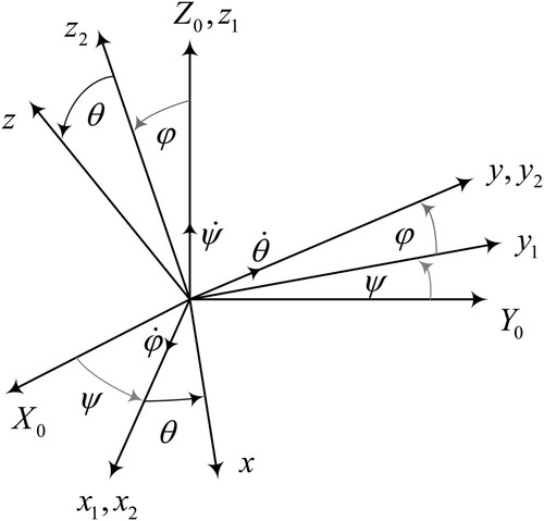
Denote by ψ the yaw angle, φ the roll angle, and ϑ the pitch angle, and put (56) $\begin{array}{r}q=\left[\begin{array}{c}\phi \\ \vartheta \\ \psi \end{array}\right],\end{array}$(56) then, when the order of rotation of the coordinate system is $Z(\psi )\to X(\phi )\to Y(\vartheta )$, the dynamical model for the spacecraft attitude system can be written in the following second-order matrix form (Duan, 2014): (57) $\begin{array}{r}M\left(q\right)\ddot{q}+D(q,\dot{q})\dot{q}+\xi (q,\dot{q})=u,\end{array}$(57) where u is the torque vector, and (58) $\begin{array}{r}M\left(q\right)=\left[\begin{array}{ccc}{I}_x\cos \vartheta & 0& -I_x\cos \phi \sin \vartheta \\ 0& I_y& I_y\sin \phi \\ I_z\sin \vartheta & 0& I_z\cos \phi \cos \vartheta \end{array}\right],\end{array}$(58) the functions $D(q,\dot{q})$ and $\xi (q,\dot{q})$ are given in the appendix. Thus the system can be rewritten in the following standard HOFA system form: (59) $\begin{array}{r}\ddot{q}=f(q,\dot{q})+B\left(q\right)u,\end{array}$(59) where (60) $\begin{array}{rl}& f(q,\dot{q})=-M^{-1}\left(q\right)[D(q,\dot{q})\dot{q}+\xi (q,\dot{q})],\end{array}$(60) (61) $\begin{array}{rl}& B\left(q\right)=M^{-1}\left(q\right).\end{array}$(61) Note that $\begin{array}{r}detB\left(q\right)=\frac{1}{I_x{I}_y{I}_z\cos \phi },\end{array}$the above system (59(59) $\begin{array}{r}\ddot{q}=f(q,\dot{q})+B\left(q\right)u,\end{array}$(59) )–(61(61) $\begin{array}{rl}& B\left(q\right)=M^{-1}\left(q\right).\end{array}$(61) ) has the following set of singular points: (62) $\begin{array}{r}\mathbb{S}=\{\left[\begin{array}{c}\phi \\ \vartheta \\ \psi \end{array}\right]|\phi =\pm \frac{\left(2k+1\right)}{2}\pi ,k=0,1,2,\dots \}.\end{array}$(62) Clearly, the distance of $\mathbb{S}$ from the origin is $\begin{array}{r}{d}_0=\frac{\pi }{2}.\end{array}$

6.2. Optimal control design

The design objective is to stabilise the HOFA system (59(59) $\begin{array}{r}\ddot{q}=f(q,\dot{q})+B\left(q\right)u,\end{array}$(59) )–(61(61) $\begin{array}{rl}& B\left(q\right)=M^{-1}\left(q\right).\end{array}$(61) ) with a nonlinear controller in the form of (8(8) $\begin{array}{rl}u& =-B^{-1}(x_k^{(0\sim {\mu }_k-1)}{|}_{k=1\sim \eta },\zeta ,t)\\ & \times [f(x_k^{(0\sim {\mu }_k-1)}{|}_{k=1\sim \eta },\zeta ,t)-v],\end{array}$(8) ), with a particular intension of keeping the spacecraft moving smoothly and steadily. Theoretically, this requires $q,\dot{q}$ and also $\ddot{q}$ to be all as small as possible, and a proper choice of the index in the form of $J_3$ in (28(28) $\begin{array}{r}{J}_3=\frac{1}{2}{\int }_0^{\mathrm{\infty }}({\Vert y\Vert }_Q^2+{\Vert x_k^{\left({\mu }_k\right)}{|}_{k=1\sim \eta }\Vert }_R^2)\mathrm{d}t,\end{array}$(28) ) will adequately meet this need. Therefore, the optimal control problem for the system (59(59) $\begin{array}{r}\ddot{q}=f(q,\dot{q})+B\left(q\right)u,\end{array}$(59) )–(61(61) $\begin{array}{rl}& B\left(q\right)=M^{-1}\left(q\right).\end{array}$(61) ) can be well established and solved by applying Theorem 5.3.

However, in order to obtain a larger feasible set of initial values to cope with the singularity in the system, we here adopt the decoupled design idea illustrated in Subsection 5.3.2, and minimise separately the following two indices: (63) $\begin{array}{rl}{J}_a& =\frac{1}{2}{\int }_0^{\mathrm{\infty }}\left({\left({\phi }^{(0\sim 1)}\right)}^{\mathrm{T}}\left[\begin{array}{cc}{q}_1& q_0\\ q_0& q_2\end{array}\right]{\phi }^{(0\sim 1)}+{\ddot{\phi }}^2\right)\mathrm{d}t,\end{array}$(63) (64) $\begin{array}{rl}{J}_b& =\frac{1}{2}{\int }_0^{\mathrm{\infty }}({\left[\begin{array}{c}{\vartheta }^{(0\sim 1)}\\ {\psi }^{(0\sim 1)}\end{array}\right]}^{\mathrm{T}}{Q}_b\left[\begin{array}{c}{\vartheta }^{(0\sim 1)}\\ {\psi }^{(0\sim 1)}\end{array}\right]\\ & +{\left[\begin{array}{c}\ddot{\vartheta }\\ \ddot{\psi }\end{array}\right]}^{\mathrm{T}}{R}_b\left[\begin{array}{c}\ddot{\vartheta }\\ \ddot{\psi }\end{array}\right])\mathrm{d}t,\end{array}$(64) where $R_b$ is positive definite, while $Q_a=[\begin{array}{cc}{q}_1& q_0\\ q_0& q_2\end{array}]$ and $Q_b$ are semi-positive definite.

With the following controller $\begin{array}{r}u=-M\left(q\right)(f(q,\dot{q})-\left[\begin{array}{c}{v}_a\\ v_b\end{array}\right]),\end{array}$the system is turned into two separate linear subsystems: (65) $\begin{array}{r}\ddot{\phi }=v_a,\end{array}$(65) and (66) $\begin{array}{r}\left[\begin{array}{c}\ddot{\vartheta }\\ \ddot{\psi }\end{array}\right]=v_b.\end{array}$(66) Their state-space forms are, respectively, (67) $\begin{array}{r}{\dot{\phi }}^{(0\sim 1)}=\left[\begin{array}{cc}0& 1\\ 0& 0\end{array}\right]{\phi }^{(0\sim 1)}+\left[\begin{array}{c}0\\ 1\end{array}\right]v_a,\end{array}$(67) and (68) $\begin{array}{r}\left[\begin{array}{c}{\dot{\vartheta }}^{(0\sim 1)}\\ {\dot{\psi }}^{(0\sim 1)}\end{array}\right]=A_E\left[\begin{array}{c}{\vartheta }^{(0\sim 1)}\\ {\psi }^{(0\sim 1)}\end{array}\right]+B_E{v}_b,\end{array}$(68) where (69) $\begin{array}{r}{A}_E=\left[\begin{array}{cccc}0& 1& 0& 0\\ 0& 0& 0& 0\\ 0& 0& 0& 1\\ 0& 0& 0& 0\end{array}\right],B_E=\left[\begin{array}{cc}0& 0\\ 1& 0\\ 0& 0\\ 0& 1\end{array}\right].\end{array}$(69) Therefore, the controller finally designed for the system is (70) $\begin{array}{r}\{\begin{array}{l}u=-M\left(q\right)(f(q,\dot{q})-\left[\begin{array}{c}{v}_a\\ v_b\end{array}\right])\\ v_a=-K_a{\phi }^{(0\sim 1)}\\ v_b=-K_b\left[\begin{array}{c}{\vartheta }^{(0\sim 1)}\\ {\psi }^{(0\sim 1)}\end{array}\right],\end{array}\end{array}$(70) where (71) $\begin{array}{r}{K}_b=R_b^{-1}{B}_E^{\mathrm{T}}{P}_b,\end{array}$(71) with $P_b$ satisfying the Riccati equation (72) $\begin{array}{r}{A}_E^{\mathrm{T}}{P_b+P_b{A}_E-P_{b}B}_E{R}_b^{-1}{B}_E^{\mathrm{T}}{P}_b+Q_b=0,\end{array}$(72) and (73) $\begin{array}{r}{K}_a=\left[01\right]P_a=\left[p_0{p}_2\right],\end{array}$(73) with $P_a$ given by (74) $\begin{array}{r}{P}_a=\left[\begin{array}{cc}{p}_1& p_0\\ p_0& p_2\end{array}\right]\end{array}$(74) and (75) $\begin{array}{r}\{\begin{array}{l}{p}_0=\sqrt{q_1}\\ p_2=\sqrt{q_2+2p_0}\\ p_1=p_0{p}_2-q_0.\end{array}\end{array}$(75) The closed-loop system is composed of (76) $\begin{array}{r}{\dot{\phi }}^{(0\sim 1)}=\left[\begin{array}{cc}0& 1\\ -p_0& -p_2\end{array}\right]{\phi }^{(0\sim 1)}\end{array}$(76) and (77) $\begin{array}{r}\left[\begin{array}{c}{\dot{\vartheta }}^{(0\sim 1)}\\ {\dot{\psi }}^{(0\sim 1)}\end{array}\right]=(A_E-B_E{K}_b)\left[\begin{array}{c}{\vartheta }^{(0\sim 1)}\\ {\psi }^{(0\sim 1)}\end{array}\right].\end{array}$(77) In order to meet the feasibility of the system (59(59) $\begin{array}{r}\ddot{q}=f(q,\dot{q})+B\left(q\right)u,\end{array}$(59) )–(61(61) $\begin{array}{rl}& B\left(q\right)=M^{-1}\left(q\right).\end{array}$(61) ), by Theorem 5.3 it is sufficient to require the following initial value restriction: (78) $\begin{array}{r}\sqrt{\nu \left(P_a\right)({\phi }^2\left(0\right)+{\dot{\phi }}^2\left(0\right))}<\frac{\pi }{2}.\end{array}$(78)

6.3. Simulation results

Consider a spacecraft with the following moments of inertia (Gao et al., 2013): (79) $\begin{array}{r}{I}_x=18,I_y=21,I_z=24.\end{array}$(79) The weighting matrices $Q_a$, $Q_b$ and $R_b$ are chosen to be (80) $\begin{array}{r}{Q}_a=\left[\begin{array}{cc}1& 0\\ 0& 2.5\end{array}\right],Q_b=\gamma I_4,R_b=I_2,\end{array}$(80) where γ is a positive parameter.

According to (73(73) $\begin{array}{r}{K}_a=\left[01\right]P_a=\left[p_0{p}_2\right],\end{array}$(73) ) and (74(74) $\begin{array}{r}{P}_a=\left[\begin{array}{cc}{p}_1& p_0\\ p_0& p_2\end{array}\right]\end{array}$(74) ), the matrices $K_a$ and $P_a$ are solved as (81) $\begin{array}{r}{K}_a=\left[\begin{array}{cc}1& 2.1213\end{array}\right]\end{array}$(81) and (82) $\begin{array}{r}{P}_a=\left[\begin{array}{cc}2.1213& 1\\ 1& 2.1213\end{array}\right],\end{array}$(82) respectively. In such a case, we have (83) $\begin{array}{r}\nu \left(P_a\right)=2.7836,\end{array}$(83) and hence, according to (78(78) $\begin{array}{r}\sqrt{\nu \left(P_a\right)({\phi }^2\left(0\right)+{\dot{\phi }}^2\left(0\right))}<\frac{\pi }{2}.\end{array}$(78) ), the initial values of ${\phi }^{(0\sim 1)}$ needs to satisfy (84) $\begin{array}{r}\sqrt{{\phi }^2\left(0\right)+{\dot{\phi }}^2\left(0\right)}<\mathrm{0.9415.}\end{array}$(84)

6.3.1. Attitude stabilisation

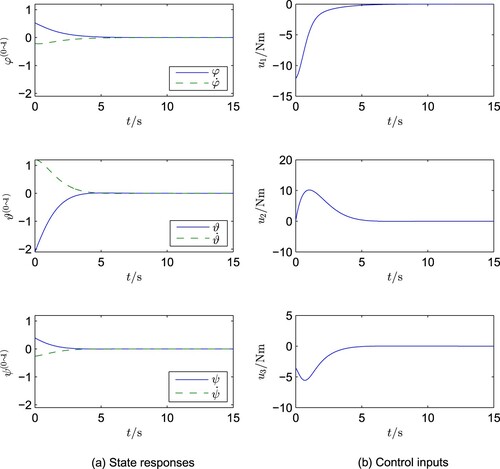
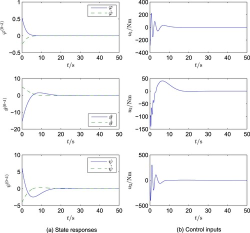
Choose $\gamma =1$, we can obtain (85) $\begin{array}{r}{P}_b=\left[\begin{array}{cccc}1.7321& 1& 0& 0\\ 1& 1.7321& 0& 0\\ 0& 0& 1.7321& 1\\ 0& 0& 1& 1.7321\end{array}\right].\end{array}$(85) hence the feedback gain can be obtained as (86) $\begin{array}{r}{K}_b=\left[\begin{array}{cccc}1& 1.7321& 0& 0\\ 0& 0& 1& 1.7321\end{array}\right].\end{array}$(86) Case A1: When the initial values are taken as (87) $\begin{array}{rl}& \phi \left(0\right)=0.5236,\dot{\phi }\left(0\right)=-0.2104,\end{array}$(87) (88) $\begin{array}{rl}& \vartheta \left(0\right)=-\frac{2}{3}\pi ,\dot{\vartheta }\left(0\right)=1.2,\end{array}$(88) and (89) $\begin{array}{r}\psi \left(0\right)=\frac{\pi }{8},\dot{\psi }\left(0\right)=-\frac{\pi }{12},\end{array}$(89) the simulation of the designed control system has been carried out and the results are shown in Figure 2.

Figure 2. Simulation results for attitude stabilisation, Case A1.

Case A2: When only the initial values in (89(89) $\begin{array}{r}\psi \left(0\right)=\frac{\pi }{8},\dot{\psi }\left(0\right)=-\frac{\pi }{12},\end{array}$(89) ) is replaced to (90) $\begin{array}{r}\psi \left(0\right)=0.9,\dot{\psi }\left(0\right)=-\frac{\pi }{4},\end{array}$(90) while keeping the other ones unchanged as in Case A1, the simulation results are shown in Figure 3.

Figure 3. Simulation results for attitude stabilisation, Case A2.

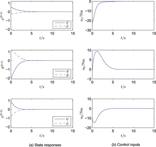
The simulation results clearly indicate the following:

1. as desired, in both cases the control technique provides very smooth and steady system responses and

2. a slight change in the initial values ${\psi }^{(0\sim 1)}(0)$ causes a big change in the corresponding control input $u_1.$

The above second phenomenon reflects the difference between nonlinear and linear systems. The reason lies in the fact that, although the two closed-loop linear subsystems are decoupled, all the control inputs are still closely coupled via the $f(\cdot )$ function.

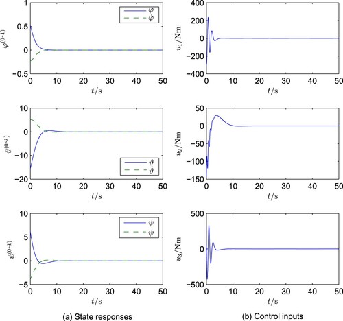
6.3.2. Rapid turning elimination

In this section, we testify the turning elimination control of the spacecraft. Let us assume that the spacecraft is turning in the θ and ψ directions with very high rates. Specifically, this is reflected in the following choice of the initial values: (91) $\begin{array}{rl}& \phi \left(0\right)=0.5236,\dot{\phi }\left(0\right)=-0.2104,\end{array}$(91) (92) $\begin{array}{rl}& \vartheta \left(0\right)=-5\pi ,\dot{\vartheta }\left(0\right)=5,\end{array}$(92) and (93) $\begin{array}{r}\psi \left(0\right)=2\pi ,\dot{\psi }\left(0\right)=-4.\end{array}$(93) With such big initial values, it is impractical to stop the turning of the spacecraft within too short time. Therefore, we decrease the weighting matrix $Q_b$ in (80(80) $\begin{array}{r}{Q}_a=\left[\begin{array}{cc}1& 0\\ 0& 2.5\end{array}\right],Q_b=\gamma I_4,R_b=I_2,\end{array}$(80) ) by reducing the factor γ.

Case B1. In the case of $\gamma =0.1,$ we can obtain (94) $\begin{array}{r}{K}_b=\left[\begin{array}{cccc}0.3162& 0.8558& 0& 0\\ 0& 0& 0.3162& 0.8558\end{array}\right],\end{array}$(94) and the simulation results are shown in Figure 4.

Figure 4. Simulation results for turning elimination, Case B1.

Case B2. In the case of $\gamma =0.01,$ we can obtain (95) $\begin{array}{r}{K}_b=\left[\begin{array}{cccc}0.1& 0.4583& 0& 0\\ 0& 0& 0.1& 0.4583\end{array}\right],\end{array}$(95) and the corresponding simulation results are shown in Figure 5.

Figure 5. Simulation results for turning elimination, Case B2.

It is clearly seen from Figures 4 and 5 the following:

1. Very effective rapid turning elimination in both Cases B1 and B2 is achieved with smooth transient process. Particularly, the turning in Case B1 is stopped in approximately 10 seconds, and that in Case B2 is stopped in approximately 25 seconds.

2. In both cases, the control amplitudes required are still in a reasonable range. The control amplitude can be accordingly reduced if the time required to stop the turning is relaxed.

7. Conclusion

Except the well-known linear quadratic optimal control technique, general nonlinear optimal control in the state–space framework still remains a big problem in the field of systems and control. Theoretical results are difficult to apply in practice due to certain nonlinear equations involved.

Parallel to the state–space approaches, HOFA approaches have been recently proposed and demonstrated to be much more effective in dealing with system control problems (Duan, 2020a, 2020b, 2020c) and (Duan, 2020d, 2020e, 2020f, 2020g, 2020h, 2020i, 2020j). It is further shown in this paper that, with the proposed HOFA approach, a type of general nonlinear optimal control can be well proposed and solved.

The problem is formulated to minimise an index in a quadratic form of the state and its derivatives of certain orders. It is shown that, with the help of the full-actuation feature of the HOFA models, the problem is linked to an optimal control problem of a linear system. Therefore, a nonlinear state feedback optimal controller can then be easily solved based on the solution to a Riccati differential or algebraic equation.

It is also shown that the formulation can be conveniently generalised to the case of sub-fully actuated systems. It turns out that the feasibility of the controller can be met by only restricting the system initial values to be within a proper ball area.

Spacecraft attitude systems are highly nonlinear ones when the attitude angles are not restricted to vary within very small ranges. Therefore, spacecraft attitude control with smooth and steady transient processes and accurate attitude manoeuvring has always remained a very hard problem. The proposed approach has been demonstrated to provide a very effective and simple way to handle such nonlinear spacecraft attitude control problems.

The results in this paper can be extended to other types of systems, e.g. discrete-time systems and uncertain systems. In addition, how to reduce the control magnitude in nonlinear optimal control certainly remains a very difficult problem.

Acknowledgments

The author is grateful to his Ph.D. students Guangtai Tian, Qin Zhao, Xiubo Wang, Weizhen Liu, Kaixin Cui, and Liyao Hu, and also his visiting scholar, Prof. Yang Cui, for helping him with reference selection and proofreading. His particular thanks go to his students Bin Zhou and Tianyi Zhao for their useful suggestions and help with the simulations, respectively.

Disclosure statement

No potential conflict of interest was reported by the author(s).

Additional information

Funding

This work has been partially supported by the Major Program of National Natural Science Foundation of China [grant numbers 61690210, 61690212], the National Natural Science Foundation of China [grant number 61333003] and the Self-Planned Task of State Key Laboratory of Robotics and System (HIT) [grant number SKLRS201716A].

Notes on contributors

Guangren Duan

Guangren Duan received his Ph.D. degree in Control Systems Sciences from Harbin Institute of Technology, Harbin, P. R. China, in 1989. After a 2-year post-doctoral experience at the same university, he became professor of control systems theory at that university in 1991. He is the founder and currently the director of the Center for Control Theory and Guidance Technology at Harbin Institute of Technology. He visited the University of Hull, the University of Sheffield, and also the Queen's University of Belfast, UK, from December 1996 to October 2002, and has served as Member of the Science and Technology committee of the Chinese Ministry of Education, Vice President of the Control Theory and Applications Committee, Chinese Association of Automation (CAA), and Associate Editors of a few international journals. He is currently an academician of the Chinese Academy of sciences, and fellow of CAA, IEEE and IET. His main research interests include parametric control systems design, nonlinear systems, descriptor systems, spacecraft control and magnetic bearing control. He is the author and co-author of 5 books and over 270 SCI indexed publications.

Appendix. Other terms in model (57)

The terms $\xi (q,\dot{q})$ and $D(q,\dot{q})$ in the spacecraft attitude system (57(57) $\begin{array}{r}M\left(q\right)\ddot{q}+D(q,\dot{q})\dot{q}+\xi (q,\dot{q})=u,\end{array}$(57) ) are given by (A1) $\begin{array}{r}\xi (q,\dot{q})=\left[\begin{array}{c}{\omega }_0^2(I_z-I_y){\pi }_x\\ {\omega }_0^2(I_x-I_z){\pi }_y\\ {\omega }_0^2(I_y-I_x){\pi }_z\end{array}\right]\end{array}$(A1) and (A2) $\begin{array}{r}D(q,\dot{q})=\left[\begin{array}{ccc}{D}_1(q,\dot{q})& D_2(q,\dot{q})& D_3(q,\dot{q})\end{array}\right],\end{array}$(A2) with (A3) $\begin{array}{rl}{D}_1(q,\dot{q})& =\left[\begin{array}{c}(I_x+I_z-I_y){\pi }_{x\phi }\\ I_y{\pi }_{y\phi }^a+(I_x-I_z){\pi }_{y\phi }^b\\ (I_x+I_z-I_y){\pi }_{z\phi }\end{array}\right],\end{array}$(A3) (A4) $\begin{array}{rl}{D}_2(q,\dot{q})& =\left[\begin{array}{c}(I_x+I_y-I_z){\pi }_{x\vartheta }\\ 0\\ (I_z+I_y-I_x){\pi }_{z\vartheta }\end{array}\right],\end{array}$(A4) (A5) $\begin{array}{rl}{D}_3(q,\dot{q})& =\left[\begin{array}{c}{I}_x{\omega }_0{\pi }_{x\psi }^a+(I_z-I_y){\pi }_{x\psi }^b\\ I_y{\omega }_0{\pi }_{y\psi }^a+(I_x-I_z){\pi }_{y\psi }^b\\ I_x{\pi }_{z\psi }^a+(I_y-I_x){\pi }_{z\psi }^b\end{array}\right],\end{array}$(A5) where in the above series of equations, (A6) $\begin{array}{r}{\omega }_0=7.292115\times {10}^{-5},\end{array}$(A6) is the rotational-angular velocity of the earth, and the set of π- functions appeared are given by (A7) $\begin{array}{rl}& \{\begin{array}{rl}{\pi }_{x\phi }=& \vartheta \sin \vartheta +\dot{\psi }\sin \phi \sin \vartheta \\ & -{\omega }_0\cos \phi \sin \vartheta \cos \psi \\ {\pi }_{x\vartheta }=& {\omega }_0\sin \vartheta \sin \psi -\dot{\psi }\cos \phi \cos \vartheta \\ & -{\omega }_0\sin \phi \cos \vartheta \cos \psi \\ {\pi }_{x\psi }^a=& \sin \phi \sin \vartheta \sin \psi -\cos \vartheta \cos \psi \\ {\pi }_{x\psi }^b=& \dot{\psi }\sin \phi \cos \phi \cos \vartheta -{\omega }_0\sin \phi \sin \vartheta \sin \psi \\ & +{\omega }_0{\sin }^2\phi \cos \vartheta \cos \psi \\ & -{\omega }_0{\cos }^2\phi \cos \vartheta \cos \psi \\ {\pi }_{x0}=& \cos \phi \sin \vartheta \sin \psi \cos \psi \\ & -\sin \phi \cos \phi \cos \vartheta {\cos }^2\psi \\ {\pi }_x=& {\pi }_{x0}-\frac{3}{2}\sin 2\phi \cos \vartheta ,\end{array}\end{array}$(A7) (A8) $\begin{array}{rl}& \{\begin{array}{rl}{\pi }_{y\phi }^a=& {\omega }_0\sin \phi \cos \psi +\dot{\psi }\cos \phi \\ {\pi }_{y\phi }^b=& \dot{\psi }\cos \phi {\cos }^2\vartheta -\dot{\psi }\cos \phi {\sin }^2\vartheta \\ & +\dot{\phi }\sin \vartheta \cos \vartheta +{\omega }_0\sin \phi {\cos }^2\vartheta \cos \psi \\ & -{\omega }_0\sin \phi {\sin }^2\vartheta \cos \psi -2{\omega }_0\sin \vartheta \sin \psi \cos \vartheta \\ {\pi }_{y\psi }^a=& \cos \phi \sin \psi \\ {\pi }_{y\psi }^b=& {\omega }_0\cos \phi {\sin }^2\vartheta \sin \psi -{\omega }_0\cos \phi {\cos }^2\vartheta \sin \psi \\ & -\dot{\psi }{\cos }^2\phi \cos \vartheta \sin \vartheta \\ & -2{\omega }_0\sin \phi \sin \vartheta \cos \phi \cos \vartheta \cos \psi \\ {\pi }_{y0}=& \cos \vartheta \sin \vartheta {\sin }^2\psi +\sin \phi {\sin }^2\vartheta \sin \psi \cos \psi -\sin \phi \\ & \times {\cos }^2\vartheta \cos \psi \sin \psi -{\sin }^2\phi \sin \vartheta \cos \vartheta {\cos }^2\psi \\ {\pi }_y=& {\pi }_{y0}+\frac{3}{2}{\cos }^2\phi \sin 2\vartheta ,\end{array}\end{array}$(A8)

and (A9) $\begin{array}{r}\{\begin{array}{rl}{\pi }_{z\phi }=& {\omega }_0\cos \phi \cos \vartheta \cos \psi -\dot{\psi }\sin \phi \cos \vartheta \\ {\pi }_{z\vartheta }=& \dot{\phi }\cos \vartheta -\dot{\psi }\cos \phi \sin \vartheta -{\omega }_0\cos \vartheta \sin \psi \\ & -{\omega }_0\sin \phi \sin \vartheta \cos \psi \\ {\pi }_{z\psi }^a=& -{\omega }_0\sin \vartheta \cos \psi -{\omega }_0\sin \phi \cos \vartheta \sin \psi \\ {\pi }_{z\psi }^b=& {\omega }_0{\cos }^2\phi \sin \vartheta \cos \psi -\dot{\psi }\sin \phi \cos \phi \sin \vartheta \\ & -{\omega }_0\sin \phi \cos \vartheta \sin \psi -{\omega }_0{\sin }^2\phi \sin \vartheta \cos \psi \\ {\pi }_{z0}=& \cos \phi \cos \vartheta \cos \psi \sin \psi +\cos \phi \sin \phi \sin \vartheta {\cos }^2\psi \\ {\pi }_z=& {\pi }_{z0}+\frac{3}{2}\sin 2\phi \sin \vartheta .\end{array}\end{array}$(A9)

References

- Abo-Sinna, M. A. (2004). Multiple objective (fuzzy) dynamic programming problems: A survey and some applications. Applied Mathematics and Computation, 157(3), 861–888. https://doi.org/https://doi.org/10.1016/j.amc.2003.08.083
- Agrawal, O. P. (2006). A formulation and a numerical scheme for fractional optimal control problems. IFAC Proceedings Volumes, 39(11), 68–72. https://doi.org/https://doi.org/10.3182/20060719-3-PT-4902.00011
- Anderson, B. D. O., & Moore, J. B. (1990). Optimal control: Linear quadratic methods. Prentice Hall.
- Arutyunov, A. V., Karamzin, D. Y., & Pereira, F. (2012). Pontryagin's maximum principle for constrained impulsive control problems. Nonlinear Analysis: Theory, Methods and Applications, 75(3), 1045–1057. https://doi.org/https://doi.org/10.1016/j.na.2011.04.047
- Ball, J. A., & Helton, J. W. (1990). Nonlinear H ∞ control theory: A literature survey. In Robust Control of Linear Systems and Nonlinear Control (pp. 1–12). Birkhäuser.
- Bellman, R. (1952). On the theory of dynamic programming. Proceedings of the National Academy of Sciences of the United States of America, 38(8), 716–719. https://doi.org/https://doi.org/10.1073/pnas.38.8.716
- Bellman, R., & Kalaba, R. (1957). On the role of dynamic programming in statistical communication theory. IRE Transactions on Information Theory, 3(3), 197–203. https://doi.org/https://doi.org/10.1109/TIT.1957.1057416
- Bellman, R., & Kalaba, R. (1960). Dynamic programming and adaptive processes: Mathematical foundation. IRE Transactions on Automatic Control, 5(1), 5–10. https://doi.org/https://doi.org/10.1109/TAC.1960.6429288
- Bender, D. J., & Laub, A. J. (1987a). The linear-quadratic optimal regulator for descriptor systems. IEEE Transactions on Automatic Control, 32(8), 672–688. https://doi.org/https://doi.org/10.1109/TAC.1987.1104694
- Bender, D. J., & Laub, A. J. (1987b). The linear-quadratic optimal regulator for descriptor systems: Discrete-time case. Automatica, 23(1), 71–85. https://doi.org/https://doi.org/10.1016/0005-1098(87)90119-1
- Bertsekas, D. P., & Tsitsiklis, J. N. (1995, December). Neuro-dynamic programming: An overview. Proceedings of 1995 34th IEEE Conference on Decision and Control (pp. 560–564). IEEE.
- Bokov, G. V. (2011). Pontryagin's maximum principle of optimal control problems with time-delay. Journal of Mathematical Sciences, 172(5), 623–634. https://doi.org/https://doi.org/10.1007/s10958-011-0208-y
- Chen, S., Li, X., & Zhou, X. Y. (1998). Stochastic linear quadratic regulators with indefinite control weight costs. SIAM Journal on Control and Optimization, 36(5), 1685–1702. https://doi.org/https://doi.org/10.1137/S0363012996310478
- Chmielewski, D., & Manousiouthakis, V. (1996). On constrained infinite-time linear quadratic optimal control. Systems & Control Letters, 29(3), 121–129. https://doi.org/https://doi.org/10.1016/S0167-6911(96)00057-6
- Çimen, T. (2008). State-dependent Riccati equation (SDRE) control: A survey. IFAC Proceedings Volumes, 41(2), 3761–3775. https://doi.org/https://doi.org/10.3182/20080706-5-KR-1001.00635
- Çimen, T. (2012). Survey of state-dependent Riccati equation in nonlinear optimal feedback control synthesis. Journal of Guidance, Control, and Dynamics, 35(4), 1025–1047. https://doi.org/https://doi.org/10.2514/1.55821
- Dmitruk, A. V., & Kaganovich, A. M. (2008). The hybrid maximum principle is a consequence of pontryagin maximum principle. Systems & Control Letters, 57(11), 964–970. https://doi.org/https://doi.org/10.1016/j.sysconle.2008.05.006
- Doyle, J., Glove, K., Khargonekar, P., & Francis, B. A. (1988). State-space solutions to standard H 2 and H ∞ control problems. In 1988 American control conference (pp. 1691–1696).
- Duan, G. R. (2014, July). Satellite attitude control–a direct parametric approach. Proceeding of the 11th World Congress on intelligent control and automation (pp. 3989–3996). IEEE.
- Duan, G. R. (2016). Linear system theory (Volume II) (3rd ed). The Science Press.
- Duan, G. R. (2020a). High-order system approaches: I. Full-actuation and parametric design. Acta Automatica Sinica, 46(7), 1333–1345. https://doi.org/https://doi.org/10.16383/j.aas.c200234 (in Chinese)
- Duan, G. R. (2020b). High-order system approaches: II. Controllability and fully-actuation. Acta Automatica Sinica, 46(8), 1571–1581. https://doi.org/https://doi.org/10.16383/j.aas.c200369 (in Chinese)
- Duan, G. R. (2020c). High-order system approaches: III. Observability and observer design. Acta Automatica Sinica, 46(9), 1885–1895. https://doi.org/https://doi.org/10.16383/j.aas.c200370 (in Chinese)
- Duan, G. R. (2020d). High-order fully actuated system approaches: Part I. Models and basic procedure. International Journal of System Sciences, 52(2), 422–435. https://doi.org/https://doi.org/10.1080/00207721.2020.1829167
- Duan, G. R. (2020e). High-order fully actuated system approaches: Part II. Generalized strict-feedback systems. International Journal of System Sciences, 52(3), 437–454. https://doi.org/https://doi.org/10.1080/00207721.2020.1829168
- Duan, G. R. (2020f). High-order fully actuated system approaches: Part III. Robust control and high-order backstepping. International Journal of System Sciences, 52(5), 952–971. https://doi.org/https://doi.org/10.1080/00207721.2020.1849863
- Duan, G. R. (2020g). High-order fully actuated system approaches: Part IV. Adaptive control and high-order backstepping. International Journal of System Sciences, 52(5), 972–989. https://doi.org/https://doi.org/10.1080/00207721.2020.1849864
- Duan, G. R. (2020h). High-order fully actuated system approaches: Part V. Robust adaptive control. International Journal of System Sciences. https://doi.org/https://doi.org/10.1080/00207721.2021.1879964
- Duan, G. R. (2020i). High-order fully actuated system approaches: Part VI. Disturbance attenuation and decoupling. International Journal of System Sciences. https://doi.org/https://doi.org/10.1080/00207721.2021.1879966
- Duan, G. R. (2020j). High-order fully actuated system approaches: Part VII. Controllability, stabilizability and parametric designs. International Journal of System Sciences. https://doi.org/https://doi.org/10.1080/00207721.2021.1921307
- Findeisen, R., Imsland, L., Allgower, F., & Foss, B. A. (2003). State and output feedback nonlinear model predictive control: an overview. European Journal of Control, 9(2–3), 190–206. https://doi.org/https://doi.org/10.3166/ejc.9.190-206
- Gao, C. Y., Zhao, Q., & Duan, G. R. (2013). Robust actuator fault diagnosis scheme for satellite attitude control systems. Journal of Franklin Institute, 350(9), 2560–2580. https://doi.org/https://doi.org/10.1016/j.jfranklin.2013.02.021
- Garcia, C. E., Prett, D. M., & Morari, M. (1989). Model predictive control: theory and practice – A survey. Automatica, 25(3), 335–348. https://doi.org/https://doi.org/10.1016/0005-1098(89)90002-2
- Hwang, C. L., & Fan, L. T. (1967). A discrete version of Pontryagin's maximum principle. Operations Research, 15(1), 139–146. https://doi.org/https://doi.org/10.1287/opre.15.1.139
- Kalman, R. E. (1960). Contributions to the theory of optimal control. Boletín De La Sociedad Matemática Mexicana, 5(2), 102–119. https://doi.org/https://doi.org/10.1109/9780470544334.ch8
- Laschov, D., & Margaliot, M. (2011a). A maximum principle for single-input Boolean control networks. IEEE Transactions on Automatic Control, 56(4), 913–917. https://doi.org/https://doi.org/10.1109/TAC.2010.2101430
- Laschov, D., & Margaliot, M. (2011b). A Pontryagin maximum principle for multi-input Boolean control networks. In Recent advances in dynamics and control of neural networks. Cambridge Scientific Publishers.
- Lee, J. H. (2011). Model predictive control: review of the three decades of development. International Journal of Control, Automation and Systems, 9(3), 415–424. https://doi.org/https://doi.org/10.1007/s12555-011-0300-6
- Lewis, F. L., & Vrabie, D. (2009). Reinforcement learning and adaptive dynamic programming for feedback control. IEEE Circuits and Systems Magazine, 9(3), 32–50. https://doi.org/https://doi.org/10.1109/MCAS.7384
- Li, Y., & Chen, Y. Q. (2008, October). Fractional order linear quadratic regulator. 2008 IEEE/ASME international conference on mechtronic and embedded systems and applications (pp. 363–368). IEEE. https://doi.org/https://doi.org/10.1109/MESA.2008.4735696
- Li, W., & Todorov, E. (2004, August). Iterative linear quadratic regulator design for nonlinear biological movement systems. ICINCO 2004 Proceedings of the first international conference on informatics in control, automation and robotics, Setúbal, Portugal (pp. 222–229). Springer.
- Mayne, D. Q. (2014). Model predictive control: recent developments and future promise. Automatica, 50(12), 2967–2986. https://doi.org/https://doi.org/10.1016/j.automatica.2014.10.128
- Nekoo, S. R. (2019). Tutorial and review on the state-dependent Riccati equation. Journal of Applied Nonlinear Dynamics, 8(2), 109–166. https://doi.org/https://doi.org/10.5890/JAND.2019.06.001
- Pontiyagin, L. S., Boltyanskii, V. G., Gamkrelidze, R. V., & Mjshchenko, E. F. (1962). The mathematical theory of optimal processes. John Wiley and Sons.
- Rami, M. A., Chen, X., & Zhou, X. Y. (2002). Discrete-time indefinite LQ control with state and control dependent noises. Journal of Global Optimization, 23(3-4), 245–265. https://doi.org/https://doi.org/10.1023/A:1016578629272
- Rozonoer, L. I. (1959). The maximum principle of LS Pontryagin in optimal system theory. Automation and Remote Control, 20(10), 11.
- Scokaert, P. O. M., & Rawlings, J. B. (1998). Constrained linear quadratic regulation. IEEE Transactions on Automatic Control, 43(8), 1163–1169. https://doi.org/https://doi.org/10.1109/9.704994
- Seierstad, A. (1975). An extension to Banach space of Pontryagin's maximum principle. Journal of Optimization Theory and Applications, 17(3-4), 293–335. https://doi.org/https://doi.org/10.1007/BF00933882
- Sussmann, H. J. (1999, December). A maximum principle for hybrid optimal control problems. Proceedings of the 38th IEEE conference on decision and control (pp. 425–430). IEEE. https://doi.org/https://doi.org/10.1109/CDC.1999.832814
- Terra, M. H., Cerri, J. P., & Ishihara, J. Y. (2014). Optimal robust linear quadratic regulator for systems subject to uncertainties. IEEE Transactions on Automatic Control, 59(9), 2586–2591. https://doi.org/https://doi.org/10.1109/TAC.2014.2309282
- Tsitsiklis, J. N., & Roy, B. V. (1997). An analysis of temporal-difference learning with function approximation. IEEE Transactions on Automatic Control, 42(5), 674–690. https://doi.org/https://doi.org/10.1109/9.580874
- Wang, L., Peng, H., Zhu, H., & Shen, L. (2009, August). A survey of approximate dynamic programming. 2009 international conference on intelligent human-machine systems and cybernetics, Hangzhou, China (pp. 396–399). IEEE.
- Werbos, P. J. (1977). Advanced forecasting methods for global crisis warning and models of intelligence. General System Yearbook, 22, 25–38.
- Werbos, P. J. (1989, August). Neural networks for control and system identification. Proceedings of the 28th IEEE conference on decision and control, Tampa, FL, USA (pp. 260–265). IEEE.
- Xie, L., & C. E. de Souza (1990). Robust H ∞ control for linear time-invariant systems with norm-bounded uncertainty in the input matrix. Systems & Control Letters, 14(5), 389–396. https://doi.org/https://doi.org/10.1016/0167-6911(90)90088-C
- Xu, S. Y., & Chen, T. W. (2002). Robust H-infinity control for uncertain stochastic systems with state delay. IEEE Transactions on Automatic Control, 47(12), 2089–2094. https://doi.org/https://doi.org/10.1109/TAC.2002.805670
- Xu, S., Yang, C., & Zhou, S. (2000). Robust H ∞ control for uncertain discrete-time systems with circular pole constraints. Systems & Control Letters, 39(1), 13–18. https://doi.org/https://doi.org/10.1016/S0167-6911(99)00066-3
- Zhang, W., Hu, J., & Abate, A. (2009). On the value functions of the discrete-time switched LQR problem. IEEE Transactions on Automatic Control, 54(11), 2669–2674. https://doi.org/https://doi.org/10.1109/TAC.2009.2031574
- Zhang, W., Hu, J., & Abate, A. (2012). Infinite-horizon switched LQR problems in discrete time: A suboptimal algorithm with performance analysis. IEEE Transactions on Automatic Control, 57(7), 1815–1821. https://doi.org/https://doi.org/10.1109/TAC.2011.2178649