A regularised fast recursive algorithm for fraction model identification of nonlinear dynamic systems

Abstract

The fraction model has been widely used to represent a range of engineering systems. To accurately identify the fraction model is however challenging, and this paper presents a regularised fast recursive algorithm (RFRA) to identify both the true fraction model structure and the associated unknown model parameters. This is achieved first by transforming the fraction form to a linear combination of nonlinear model terms. Then the terms in the denominator are used to form a regularisation term in the cost function to offset the bias induced by the linear transformation. According to the structural risk minimisation principle based on the new cost function, the model terms are selected based on their contributions to the cost function and the coefficients are then identified recursively without explicitly solving the inverse matrix. The proposed method is proved to have low computational complexity. Simulation results confirm the efficacy of the method in fast identification of the true fraction models for the targeted nonlinear systems.

Keywords:

• Regularisation
• fraction models
• regularised fast recursive algorithm
• nonlinear model identification

1. Introduction

Machine learning is a powerful tool for technological progress and has been widely adopted for approximating nonlinear dynamic systems (Yildiz et al., 2017). The nonlinear system modelling has been a subject of intensive research in the past decades, and various machine learning regression (Singh & Dhiman, 2021) models have been proposed, such as polynomial nonlinear models (Paduart et al., 2010; Wang et al., 2021; C. Yang et al., 2020), rational models (Austin et al., 2021; Zhu et al., 2015, 2019), support vector machine (SVM) based regression models (Liang & Zhang, 2021; Suykens et al., 2002) and neural network models (Du et al., 2022; Qiao et al., 2018; Z. Yang et al., 2020), to just name a few.

Among them, polynomial nonlinear regression models are the most popular machine learning regression methods due to their simplicity to develop and capture complex relationships between system inputs and system outputs (Gambella et al., 2021). In particular, the rational model which is a ratio of two polynomials has attracted more attentions in the community as many engineering systems can be modelled as the ratio of two linear-in-the-parameter equations (Andreev & Borulko, 2017; Curtain & Morris, 2009; Hussein & Batarseh, 2011; Kambhampati et al., 2000; Swarnakar et al., 2017, Dec; Zhu et al., 2019), each consisting of some base functions. They are often referred to fraction models, and the rational models which all consist of polynomial terms in both numerator and denominator is a special case (Li, 2005). The fraction model has the capability of concisely approximating a wide range of nonlinear systems, while traditional models such as nonlinear polynomial ARX models, neural networks, support vector machines (SVM) (J. Zhang et al., 2012) may become overly complex in order to achieve the same level of modelling accuracy.

To fit a fraction model using the training data is a machine learning regression modelling problem. To establish an accurate fraction model, an efficient automatic learning method is the key to both determine the model structure and identify unknown parameters. This is however technically challenging, and for rational models as a special case, the solutions fall into two major categories. The first one is to transform the rational form to a linear-in-the-parameter expression (Billings & Zhu, 1991, 1994). Based on the transformed system, various algorithms have been developed to identify a suitable model structure and in the meantime to identify the unknown linear coefficients (Billings & Mao, 1998; Billings & Zhu, 1991; Zhu, 2003, 2005; Zhu & Billings, 1996; Zhu et al., 2017). These algorithms all have the same aim to iteratively offset the bias by updating the coefficients and the regressors based on the variance of estimation errors. The resultant models identified by these well-established methods are often less complex, though they still suffer from high computation complexity. The other approach is directly selecting the base function using the orthogonal methods, such as an orthogonal rational model estimation (Billings & Zhu, 1994) and Stieltjes process (Austin et al., 2021).

In particular, the popular orthogonal least square (OLS) method has been widely used for identifying a range of nonlinear models including the rational models (Zhu & Billings, 1996) although the conventional OLS scheme is still computationally expensive, particularly for backward model reduction. To reduce the computational complexity, Li et al proposed a fast recursive algorithm (FRA) (Li et al., 2005). The FRA framework has further led to the development of a series of effective algorithms for nonlinear system modelling, such as the two-stage stepwise algorithm (Li et al., 2006), two-stage OLS method (L. Zhang et al., 2015), least squares support vector machine (LSSVM) (Zhao et al., 2015) as well as methods to construct compact RBF networks (Deng et al., 2012, 2013, 2010). This paper will use the similar algorithmic framework to build fraction models for nonlinear systems, aiming to both develop a compact model and reduce the computational complexity.

A challenge for identifying the fraction model is to eliminate the bias caused by the errors introduced by the transformation. To tackle this challenge, various methods have been proposed to estimate the errors (J. Chen et al., 2018; Jin & Weng, 2019; Manela & Biess, 2021; Piga & Tóth, 2014). In order to penalise the bias induced by the linear transformation, this paper adopts a negative regularisation term to penalise the errors introduced into the transformed linear model. In essence, the regularisation term is used to balance the linear model estimation error and the bias of the estimated parameters due to the linear transformation (Ohlsson et al., 2010). The regularisation method proposed by Tikhonov (Tikhonov & Glasko, 1965) and its variants (Luo et al., 2016; Münker & Nelles, 2016; L. Zhang et al., 2019) have been widely used in machine learning to reduce the bias introduced into the parameter estimation. Popular regularisation methods include the ${\ell }_0$ regularisation, ${\ell }_1$ regularisation and ${\ell }_2$ regularisation (Castella et al., 2018; Luo et al., 2016; Senhaji et al., 2020; Tao et al., 2015; Torres-Barrán et al., 2018) where the weight of the regularisation term is often set positive to avoid over-fitting, while in this paper a negative weight is applied to the penalty term to reduce the bias introduced by the linear transformation. However, the weight has to be sufficiently small to ensure that the contributions to the cost function are positive.

Within the regularisation framework, to choose a suitable regularisation term is critical, and a number of kernel functions have been used to define the regularisation term (Birpoutsoukis et al., 2017; T. Chen et al., 2014; Pillonetto, 2018). The kernel method which performs a nonlinear data transformation has been widely applied in system identification, machine learning and function estimation (Bai et al., 2014; T. Chen et al., 2014; Hofmann et al., 2008; Pillonetto & De Nicolao, 2010; Pillonetto et al., 2014). Reproducing kernel Hilbert spaces (RKHSs) (Pillonetto et al., 2014; Valencia & lvarez, 2017) is a popular one. Similarly, in this paper, the inner product of nonlinear mapping terms in the denominator is added to the cost function with the aim to reduce the bias caused by the linear transformation. The effectiveness of this treatment will be assessed in the simulation section.

Given the quadratic cost function as a trade-off between the linear model error and model parameters bias caused by linear transformation, a regularised fast recursive algorithm is proposed in this paper to solve the optimisation problem. The main contributions in this paper are summarised as follows:

• A duality formulation is introduced to translate the fraction model identification problem to a quadratic linear regression problem. Based on the structural risk minimisation principle, the dual linear regression problem is minimised by a variant of the least squares solution. In essence, identification of a fraction model is thus translated to solving a linear regression problem, thus significantly reduced the computational complexity.

• To eliminate the bias induced by the linear-in-the-parameters transformation and to recover the true fraction model rather than identify a parsimonious model, a regularisation term is added to the cost function. The optimisation problem can be easily solved by a regularised least-squares method.

• To automatically identify both the fraction model coefficients and the fraction model structure, a regularised fast approach (RFRA) is proposed based on the original fast recursive algorithm (Li et al., 2005). Unlike the locally regularised automatic construction (LRAC) method (Du et al., 2012), the regularisation matrix does not have to be a diagonal matrix when using the novel regularised fast recursive method. In order to efficiently evaluate the candidate base function, a recursive net contribution is developed. The proposed RFRA method simplifies the calculation of the net contribution of model terms and computation of the least squares equations for the coefficients by defining a set of recursive matrices, and the fraction model structure is determined according to the net contribution easily.

• Finally, the complexity of the proposed method is analysed and compared with the well-known orthogonal method proposed in Zhu and Billings (1996) to confirm its efficiency.

The remainder of the paper is organised as follows. The fraction model identification problem is formulated in Section 2. Section 3 gives some necessary preliminaries for the proposed algorithm. Then a regularised fast method is detailed in Section 4, covering the principle of the new method, fast computation of the net contribution of model terms, fast computation of model coefficients, and computational complexity analysis. Simulation case studies are presented in Section 5. Finally, Section 6 concludes this paper.

2. Problem formulation

2.1. Fraction model

Considering a multiple-input single-output system, the fraction model can be expressed as the ratio of two linear-in-the-parameter models. (1) $y\left(t\right)=\frac{a\left(t\right)}{c\left(t\right)}+e\left(t\right)=\frac{\sum _{i=1}^r\left[p_{ni}\right(\mathbf{\text{x}}\left(t\right))\cdot {\theta }_{ni}]}{\sum _{j=1}^h\left[p_{dj}\right(\mathbf{\text{x}}\left(t\right))\cdot {\theta }_{dj}]}+e\left(t\right)$(1) where $y\left(t\right)$, $\mathbf{\text{x}}\left(t\right)=\left[x_1\right(t),\dots ,x_q(t\left)\right]$ and $e\left(t\right)$ are the model output, the model input vector with q dimension and the model error at time instant t, respectively. $p_{ni}$ represents the ith nonlinear base mapping term of the numerator and $p_{dj}$ represents the jth nonlinear base mapping term of the denominator. r and h denote the numbers of the nonlinear terms in the numerator and in the denominator of the fraction model respectively. Also ${\theta }_{ni}$ and ${\theta }_{dj}$ represent the coefficients of the ith regressor in the numerator and the jth regressor in the denominator respectively.

To identify the fraction model from the training data, the system (1(1) $y\left(t\right)=\frac{a\left(t\right)}{c\left(t\right)}+e\left(t\right)=\frac{\sum _{i=1}^r\left[p_{ni}\right(\mathbf{\text{x}}\left(t\right))\cdot {\theta }_{ni}]}{\sum _{j=1}^h\left[p_{dj}\right(\mathbf{\text{x}}\left(t\right))\cdot {\theta }_{dj}]}+e\left(t\right)$(1) ) can be expressed in the matrix representation first. Then the cost function of the corresponding dual quadratic linear regression problem can be calculated and further simplified. Suppose N data samples $\left\{x\right(t),y(t){\}}_{t=1}^N$ are used for model identification, Equation (1(1) $y\left(t\right)=\frac{a\left(t\right)}{c\left(t\right)}+e\left(t\right)=\frac{\sum _{i=1}^r\left[p_{ni}\right(\mathbf{\text{x}}\left(t\right))\cdot {\theta }_{ni}]}{\sum _{j=1}^h\left[p_{dj}\right(\mathbf{\text{x}}\left(t\right))\cdot {\theta }_{dj}]}+e\left(t\right)$(1) ) can be formulated as (2) $\mathit{y}=\mathit{a}\oslash \mathit{c}+\mathit{e}=\left({\mathit{P}}_n{\mathbf{\Theta }}_n\right)\oslash \left({\mathit{P}}_d{\mathbf{\Theta }}_d\right)+\mathit{e}$(2) where $\mathit{y}=\left[y\right(1),\dots ,y(N){]}^{\mathrm{T}}$ is the model output vector. $\mathit{a}=\left[a\right(1),\dots ,a(N){]}^{\mathrm{T}}$ is the numerator sample vector. $\mathit{c}=\left[c\right(1),\dots ,c(N){]}^{\mathrm{T}}$ is the denominator sample vector. The components of $\mathit{a}\oslash \mathit{c}$ are $(\mathit{a}\oslash \mathit{c}{)}_l=a(l\left)/c\right(l),1=<l<=N$. $\mathit{e}=\left[e\right(1),\dots ,e(N){]}^{\left(\mathrm{T}\right)}$ is the model error vector. ${\mathit{P}}_n=[{\mathit{p}}_{n1},\dots ,{\mathit{p}}_{nr}]$ $\in {\mathrm{\Re }}^{N\times r}$ is the selected nonlinear mapping matrix for the numerator with ${\mathit{p}}_{ni}=\left[p_{ni}\right(\mathit{x}\left(1\right)),\dots$ $p_{ni}\left(\mathit{x}\right(N\left)\right){]}^{\mathrm{T}},i=1,\dots ,r$. ${\mathbf{\Theta }}_n=[{\theta }_{n1},\dots ,{\theta }_{nr}{]}^{\mathrm{T}}\in {\mathrm{\Re }}^{r\times 1}$ is the coefficients vector for the numerator. ${\mathit{P}}_d=[{\mathit{p}}_{d1},\dots ,{\mathit{p}}_{dh}]\in {\mathrm{\Re }}^{N\times h}$ is the selected nonlinear mapping matrix for the denominator with ${\mathit{p}}_{dj}=\left[p_{dj}\right(\mathit{x}\left(1\right)),\dots ,p_{dj}(\mathit{x}\left(N\right)){]}^{\mathrm{T}},$ $j=1,\dots ,h$. ${\mathbf{\Theta }}_d=[{\theta }_{d1},\dots ,{\theta }_{dh}{]}^{\mathrm{T}}\in {\mathrm{\Re }}^{h\times 1}$ is the coefficients vector for the denominator.

2.2. Transformation to linear-in-the-parameter formulation

Fraction models are not naturally linear in the parameters and its identification presents a challenge. To identify fraction models, an elementwise product of the two vectors is first defined, namely Hadamard product using ⊙ to denote the product (Nielsen, 2019). Suppose $\mathit{\alpha }$ and $\text{β}$ are two vectors of the same dimension, then the lth component of $\mathit{\alpha }\odot \text{β}$ is $(\mathit{\alpha }\odot \text{β}{)}_l=\alpha (l\left)\text{β}\right(l)$.

To obtain the matrix representation of the corresponding linear system in the sense of least squares, both sides of Equation (2(2) $\mathit{y}=\mathit{a}\oslash \mathit{c}+\mathit{e}=\left({\mathit{P}}_n{\mathbf{\Theta }}_n\right)\oslash \left({\mathit{P}}_d{\mathbf{\Theta }}_d\right)+\mathit{e}$(2) ) are Hadamard multiplied by '$\mathit{c}\in {\mathrm{\Re }}^{N\times 1}$', thus: (3) $\begin{array}{rl}\mathit{y}\odot \mathit{c}& =\mathit{a}\oslash \mathit{c}\odot \mathit{c}+\mathit{e}\odot \mathit{c}=\mathit{a}+\mathit{e}\odot \mathit{c}\\ & =\left({\mathit{P}}_n{\mathbf{\Theta }}_n\right)+\mathit{e}\odot \mathit{c}=\mathit{y}\odot \left({\mathit{P}}_d{\mathbf{\Theta }}_d\right)\end{array}$(3) Expanding ${\mathit{P}}_d{\mathbf{\Theta }}_d$ and ${\mathit{P}}_n{\mathbf{\Theta }}_n$ in (3(3) $\begin{array}{rl}\mathit{y}\odot \mathit{c}& =\mathit{a}\oslash \mathit{c}\odot \mathit{c}+\mathit{e}\odot \mathit{c}=\mathit{a}+\mathit{e}\odot \mathit{c}\\ & =\left({\mathit{P}}_n{\mathbf{\Theta }}_n\right)+\mathit{e}\odot \mathit{c}=\mathit{y}\odot \left({\mathit{P}}_d{\mathbf{\Theta }}_d\right)\end{array}$(3) ) gives (4) $\begin{array}{rl}& \mathit{y}\odot ({\mathit{p}}_{d1}\cdot {\theta }_{d1}+{\mathit{p}}_{d2}\cdot {\theta }_{d2}+\cdots +{\mathit{p}}_{dh}\cdot {\theta }_{dh})\\ & =({\mathit{p}}_{n1}\cdot {\theta }_{n1}+{\mathit{p}}_{n2}\cdot {\theta }_{n2}+\cdots +{\mathit{p}}_{nr}\cdot {\theta }_{nr})+\mathit{e}\odot \mathit{c}\end{array}$(4) Thereby, (5) $\begin{array}{rl}& \mathit{y}\odot {\mathit{p}}_{d1}\cdot {\theta }_{d1}+\mathit{y}\odot {\mathit{p}}_{d2}\cdot {\theta }_{d2}+\cdots +\mathit{y}\odot {\mathit{p}}_{dh}\cdot {\theta }_{dh}\\ & =({\mathit{p}}_{n1}\cdot {\theta }_{n1}+{\mathit{p}}_{n2}\cdot {\theta }_{n2}+\cdots +{\mathit{p}}_{nr}\cdot {\theta }_{nr})+\mathit{e}\odot \mathit{c}\end{array}$(5) Then all the terms except '$\mathit{y}\odot {\mathit{p}}_{d1}\cdot {\theta }_{d1}$' are moved to the right side, resulting in a linear-in-the-parameter model (6) $\begin{array}{rl}\mathit{y}\odot {\mathit{p}}_{d1}{\theta }_{d1}& =({\mathit{p}}_{n1}\cdot {\theta }_{n1}+{\mathit{p}}_{n2}\cdot {\theta }_{n2}+\cdots +{\mathit{p}}_{nr}\cdot {\theta }_{nr})\\ & -\mathit{y}\odot {\mathit{p}}_{d2}\cdot {\theta }_{d2}-\cdots -\mathit{y}\odot {\mathit{p}}_{dh}\cdot {\theta }_{dh}\\ & =[{\mathit{p}}_{n1},{\mathit{p}}_{n2},\dots ,{\mathit{p}}_{nr}\cdot {\theta }_{nr}]\\ & \times [{\theta }_{n1},{\theta }_{n2},\dots ,{\theta }_{nr}{]}^{\mathrm{T}}\\ & -[\mathit{y}\odot {\mathit{p}}_{d2},\cdots ,\mathit{y}\odot {\mathit{p}}_{dh}]\\ & \cdot [{\theta }_{d2},\dots ,{\theta }_{dh}{]}^{\mathrm{T}}+\mathit{e}\odot \mathit{c}\\ & =[{\mathit{p}}_{n1},\dots ,{\mathit{p}}_{nr},-\mathit{y}\odot {\mathit{p}}_{d2},\dots ,-\mathit{y}\odot {\mathit{p}}_{dh}]\\ & \times [{\theta }_{n1},\dots ,{\theta }_{nr},{\theta }_{d2},\dots ,{\theta }_{dh}{]}^{\mathrm{T}}\\ & +\mathit{e}\odot \mathit{c}\end{array}$(6) By defining $\mathit{Y}=\mathit{y}\odot {\mathit{p}}_{d1}{\theta }_{d1}$, $\mathbf{\Phi }=[{\mathit{p}}_{n1},\dots ,{\mathit{p}}_{nr},-\mathit{y}\odot {\mathit{p}}_{d2},\dots ,-\mathit{y}\odot {\mathit{p}}_{dh}]$ and $\mathbf{\Theta }=[{\theta }_{n1},\dots ,{\theta }_{nr},{\theta }_{d2},\dots ,{\theta }_{dh}{]}^{\mathrm{T}}$, the system can be reformulated as follows: (7) $\mathit{Y}=\mathbf{\Phi }\mathbf{\Theta }+\mathit{c}\odot \mathit{e}=\mathbf{\Phi }\mathbf{\Theta }+\mathbf{\Xi }$(7) where ${\theta }_{d1}$ generally takes the value of 1, ${\mathit{p}}_{d1}={\mathbf{1}}_{N\times 1}$, $\mathit{Y}=\left[y\right(1)\cdot p_{d1}(1),\dots ,y(N)\cdot p_{d1}(N){]}^{\mathrm{T}}=[y\left(1\right),\dots ,y\left(N\right){]}^{\mathrm{T}}$ is the output vector of new system, $\mathbf{\Theta }=[{\theta }_{n1},$ $\cdots ,{\theta }_{nr},{\theta }_{d2},\dots ,{\theta }_{dh}{]}^{\mathrm{T}}$ is the new system linear parameter vector, $\mathbf{\Xi }=\left[c\right(1\left)e\right(1),\dots ,$ $c\left(N\right)e\left(N\right){]}^{\mathrm{T}}$ is the coloured noise of the new system, $\mathbf{\Phi }=[{\mathit{\varphi }}_1,\dots ,$ ${\mathit{\varphi }}_M]=[{\mathit{p}}_{n1},\dots ,{\mathit{p}}_{nr},-\mathit{y}\odot {\mathit{p}}_{d2},\dots ,-\mathit{y}\odot {\mathit{p}}_{dh}]$ with M regressors for inclusion in the model, where M = r + h−1.

2.3. Model identification challenges

By transforming the fraction model in the linear-in-the-parameter form, the model identification is simplified to a linear regression problem. Both the least squares method and the likelihood estimation are two well-established methods. Here the least squares method (LS) is applied to model equation (7(7) $\mathit{Y}=\mathbf{\Phi }\mathbf{\Theta }+\mathit{c}\odot \mathit{e}=\mathbf{\Phi }\mathbf{\Theta }+\mathbf{\Xi }$(7) ) given that the distribution of the training samples is unknown prior.

For the new system formulated in Equation (7(7) $\mathit{Y}=\mathbf{\Phi }\mathbf{\Theta }+\mathit{c}\odot \mathit{e}=\mathbf{\Phi }\mathbf{\Theta }+\mathbf{\Xi }$(7) ), the input matrix and output vector of the model are $[{\mathit{x}}_1,\dots ,{\mathit{x}}_q,\mathit{y}]\in {\mathrm{\Re }}^{N\times (q+1)}$ and $\mathit{Y}\in {\mathrm{\Re }}^{N\times 1}$, respectively. 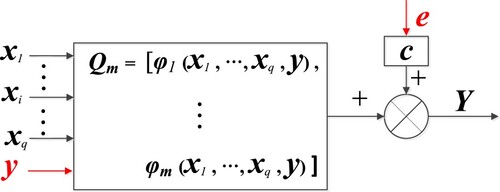Then m candidate nonlinear features ${\mathit{\phi }}_i({\mathit{x}}_1,\dots ,{\mathit{x}}_q,\mathit{y}),i=1,\dots ,m$ are generated if the true system is unknown a priori. Generally speaking, if the true model is unknown, then various parsimonious nonlinear models such as polynomial models and other linear-in-the-parameter models can be built to achieve equivalent modelling performance under certain conditions (Li & Peng, 2007). Thus, a polynomial is often used to approximate a range of nonlinear systems. To this end, ${\mathit{\phi }}_i$ can be defined as a polynomial term. If the system model is partially known a priori, then fundamental knowledge can be obtained for an engineering system (Li, 2005) based on which fundamental functions (${\mathit{\phi }}_i$) can be identified, such as exponential, fraction order polynomial terms, trigonometric, or rational functions, etc. The resultant model structure is illustrated in Figure 1.

Figure 1. The structure of the new linear-in-parameters system.

In statistics, there exists biased parameter estimators to dominate any unbiased parameter estimator in terms of the mean squared error (MSE) (Hong et al., 2008), therefore there is always a requirement to balance the variance and bias using the least square method. In LS method, the linear coefficients $\mathbf{\Theta }$ can be estimated by (8) $\stackrel{\mathbf{ˆ}}{\mathbf{\Theta }}=({\mathbf{\Phi }}^{\mathrm{T}}\mathbf{\Phi }{)}^{-1}{\mathbf{\Phi }}^{\mathrm{T}}\mathit{Y}$(8) In theory, for the linear-in-the-parameter system subject to white noise, the least square solution of the coefficients ($E\left[\stackrel{\mathbf{ˆ}}{\mathbf{\Theta }}\right]$) is equal to the true value $\mathbf{\Theta }$ if the sample number is sufficiently large. However, for the system in Equation (7(7) $\mathit{Y}=\mathbf{\Phi }\mathbf{\Theta }+\mathit{c}\odot \mathit{e}=\mathbf{\Phi }\mathbf{\Theta }+\mathbf{\Xi }$(7) ), the linear coefficients in Equation (8(8) $\stackrel{\mathbf{ˆ}}{\mathbf{\Theta }}=({\mathbf{\Phi }}^{\mathrm{T}}\mathbf{\Phi }{)}^{-1}{\mathbf{\Phi }}^{\mathrm{T}}\mathit{Y}$(8) ) can be described as (9) $\stackrel{\mathbf{ˆ}}{\mathbf{\Theta }}=\left({\mathbf{\Phi }}^{\mathrm{T}}\mathbf{\Phi }{)}^{-1}{\mathbf{\Phi }}^{\mathrm{T}}\right(\mathbf{\Phi }\mathbf{\Theta }+\mathbf{\Xi })=\mathbf{\Theta }+({\mathbf{\Phi }}^{\mathrm{T}}\mathbf{\Phi }{)}^{-1}{\mathbf{\Phi }}^{\mathrm{T}}\mathbf{\Xi }$(9) It is clear that the noise $\mathbf{\Xi }$ in Equation (9(9) $\stackrel{\mathbf{ˆ}}{\mathbf{\Theta }}=\left({\mathbf{\Phi }}^{\mathrm{T}}\mathbf{\Phi }{)}^{-1}{\mathbf{\Phi }}^{\mathrm{T}}\right(\mathbf{\Phi }\mathbf{\Theta }+\mathbf{\Xi })=\mathbf{\Theta }+({\mathbf{\Phi }}^{\mathrm{T}}\mathbf{\Phi }{)}^{-1}{\mathbf{\Phi }}^{\mathrm{T}}\mathbf{\Xi }$(9) ) comes from $\mathit{c}\odot \mathit{e}$ defined in Equation (7(7) $\mathit{Y}=\mathbf{\Phi }\mathbf{\Theta }+\mathit{c}\odot \mathit{e}=\mathbf{\Phi }\mathbf{\Theta }+\mathbf{\Xi }$(7) ), therefore it is a coloured noise. From Figure 1, $\mathbf{\Phi }$ is correlated with $\mathit{e}$ as it is included in the information of the output $\mathit{y}$. Therefore, the expectation of estimation coefficients ($E\left[\stackrel{\mathbf{ˆ}}{\mathbf{\Theta }}\right]$) is $\mathbf{\Theta }+E\left[\right({\mathbf{\Phi }}^{\mathrm{T}}\mathbf{\Phi }{)}^{-1}{\mathbf{\Phi }}^{\mathrm{T}}\mathbf{\Xi }]$ rather than $\mathbf{\Theta }$. Thus, the least square method applied to system (7(7) $\mathit{Y}=\mathbf{\Phi }\mathbf{\Theta }+\mathit{c}\odot \mathit{e}=\mathbf{\Phi }\mathbf{\Theta }+\mathbf{\Xi }$(7) ) has a bias term in the solution, and it is necessary to eliminate the bias to improve the generalisation performance of a parsimonious model or to identify the true system model from a model candidate term pool consisting of the true model terms.

From Equation (9(9) $\stackrel{\mathbf{ˆ}}{\mathbf{\Theta }}=\left({\mathbf{\Phi }}^{\mathrm{T}}\mathbf{\Phi }{)}^{-1}{\mathbf{\Phi }}^{\mathrm{T}}\right(\mathbf{\Phi }\mathbf{\Theta }+\mathbf{\Xi })=\mathbf{\Theta }+({\mathbf{\Phi }}^{\mathrm{T}}\mathbf{\Phi }{)}^{-1}{\mathbf{\Phi }}^{\mathrm{T}}\mathbf{\Xi }$(9) ), it is clear that the bias is related to the selected terms of the denominator and $\mathit{e}$. Accordingly, an improved method is proposed in the following to eliminate the bias.

3. Preliminaries

Through the linear transformation, noises have been introduced into both input and outputs of the new system (2(2) $\mathit{y}=\mathit{a}\oslash \mathit{c}+\mathit{e}=\left({\mathit{P}}_n{\mathbf{\Theta }}_n\right)\oslash \left({\mathit{P}}_d{\mathbf{\Theta }}_d\right)+\mathit{e}$(2) ). Furthermore, the output-error is a coloured noise which is the response excited by the white noise of the original system. Given the coloured noise, the conventional recursive least square method leads to a biased solution. To achieve unbiased coefficients estimation, a similar process to the reproducing kernel Hilbert space (RKHS) method (Pillonetto, 2018) which uses the inner products of the denominator is employed to mitigate the contribution of the bias to the cost function. By adding a regularisation term with a negative weight, it is possible to eliminate the bias introduced into the estimation of the original system.

3.1. The original cost function

Lemma 3.1

Suppose $\mathit{e}=\left[e\right(1),\dots ,e(N\left)\right]$ obeys a Gaussian distribution with zero mean, for given sufficient enough data samples, then Hadamard product ($(\mathit{c}\odot \mathit{e}{)}^{\mathrm{T}}(\mathit{c}\odot \mathit{e})$) satisfies: (10) $(\mathit{c}\odot \mathit{e}{)}^{\mathrm{T}}(\mathit{c}\odot \mathit{e})={\mathbf{\Xi }}^{\mathrm{T}}\mathbf{\Xi }=\frac{1}{N}\cdot {\mathit{c}}^{\mathrm{T}}\mathit{c}\cdot {\mathit{e}}^{\mathrm{T}}\mathit{e}$(10) The proof is given as follows.

According to the multiplication of matrices, the right side of Equation (10(10) $(\mathit{c}\odot \mathit{e}{)}^{\mathrm{T}}(\mathit{c}\odot \mathit{e})={\mathbf{\Xi }}^{\mathrm{T}}\mathbf{\Xi }=\frac{1}{N}\cdot {\mathit{c}}^{\mathrm{T}}\mathit{c}\cdot {\mathit{e}}^{\mathrm{T}}\mathit{e}$(10) ) can be expanded as (11) $\begin{array}{rl}{\mathit{c}}^{\mathrm{T}}\mathit{c}\cdot {\mathit{e}}^{\mathrm{T}}\mathit{e}& =\sum _{i=1}^N{c}^2\left(i\right)\sum _{j=1}^N{\mathrm{e}}^2\left(i\right)\\ & =\left(c^2\right(1)+\cdots +c^2(N\left)\right)\sum _{j=1}^N{\mathrm{e}}^2\left(j\right)\\ & =c^2\left(1\right)\sum _{j=1}^N{\mathrm{e}}^2\left(j\right)+\cdots +c^2\left(N\right)\sum _{j=1}^N{\mathrm{e}}^2\left(j\right)\\ & =(\mathit{c}\odot \mathit{e}{)}^{\mathrm{T}}(\mathit{c}\odot \mathit{e})+c^2(1\left)\sum _{j=2}^N{\mathrm{e}}^2\right(j)+\cdots \\ & +c^2\left(i\right)\sum _{j=1\mathrm{\&}j\ne i}^N{\mathrm{e}}^2\left(j\right)+\cdots \\ & +c^2\left(N\right)\sum _{j=1}^{N-1}{\mathrm{e}}^2\left(j\right)\end{array}$(11) If the system error ‘$\mathit{e}$’ is a white noise with the variance ‘${\sigma }_e^2$’, Equation (11(11) $\begin{array}{rl}{\mathit{c}}^{\mathrm{T}}\mathit{c}\cdot {\mathit{e}}^{\mathrm{T}}\mathit{e}& =\sum _{i=1}^N{c}^2\left(i\right)\sum _{j=1}^N{\mathrm{e}}^2\left(i\right)\\ & =\left(c^2\right(1)+\cdots +c^2(N\left)\right)\sum _{j=1}^N{\mathrm{e}}^2\left(j\right)\\ & =c^2\left(1\right)\sum _{j=1}^N{\mathrm{e}}^2\left(j\right)+\cdots +c^2\left(N\right)\sum _{j=1}^N{\mathrm{e}}^2\left(j\right)\\ & =(\mathit{c}\odot \mathit{e}{)}^{\mathrm{T}}(\mathit{c}\odot \mathit{e})+c^2(1\left)\sum _{j=2}^N{\mathrm{e}}^2\right(j)+\cdots \\ & +c^2\left(i\right)\sum _{j=1\mathrm{\&}j\ne i}^N{\mathrm{e}}^2\left(j\right)+\cdots \\ & +c^2\left(N\right)\sum _{j=1}^{N-1}{\mathrm{e}}^2\left(j\right)\end{array}$(11) ) can be reformulated as follows given that there are sufficient data samples. (12) $\begin{array}{rl}{\mathit{c}}^{\mathrm{T}}\mathit{c}\cdot {\mathit{e}}^{\mathrm{T}}\mathit{e}& ={\mathbf{\Xi }}^{\mathrm{T}}\mathbf{\Xi }+c^2\left(1\right)\cdot (N-1)\cdot {\sigma }_e^2+\cdots \\ & +c^2\left(i\right)\cdot (N-1)\cdot {\sigma }_e^2+\cdots \\ & +c^2\left(N\right)\cdot (N-1)\cdot {\sigma }_e^2\\ & ={\mathbf{\Xi }}^{\mathrm{T}}\mathbf{\Xi }+\sum _{i=1}^N{c}^2\left(i\right)\cdot (N-1)\cdot {\sigma }_e^2\\ & ={\mathbf{\Xi }}^{\mathrm{T}}\mathbf{\Xi }+\sum _{i=1}^N{c}^2\left(i\right)\cdot \frac{N-1}{N}{\mathit{e}}^{\mathrm{T}}\mathit{e}\\ & ={\mathbf{\Xi }}^{\mathrm{T}}\mathbf{\Xi }+\frac{N-1}{N}{\mathit{c}}^{\mathrm{T}}\mathit{c}\cdot {\mathit{e}}^{\mathrm{T}}\mathit{e}\end{array}$(12) Accordingly, Equation (10(10) $(\mathit{c}\odot \mathit{e}{)}^{\mathrm{T}}(\mathit{c}\odot \mathit{e})={\mathbf{\Xi }}^{\mathrm{T}}\mathbf{\Xi }=\frac{1}{N}\cdot {\mathit{c}}^{\mathrm{T}}\mathit{c}\cdot {\mathit{e}}^{\mathrm{T}}\mathit{e}$(10) ) is true.

Considering the coloured noise '$\mathbf{\Xi }$' in Equation (7(7) $\mathit{Y}=\mathbf{\Phi }\mathbf{\Theta }+\mathit{c}\odot \mathit{e}=\mathbf{\Phi }\mathbf{\Theta }+\mathbf{\Xi }$(7) ), the sum of squared coloured noises can be calculated as follows: (13) ${\mathbf{\Xi }}^{\mathrm{T}}\mathbf{\Xi }=\frac{{\mathit{c}}^{\mathrm{T}}\mathit{c}\cdot {\mathit{e}}^{\mathrm{T}}\mathit{e}}{N}$(13) where $\mathbf{\Xi }=\mathit{Y}-\mathbf{\Phi }\mathbf{\Theta }$ and $\mathit{e}=\mathit{y}-\mathit{a}\oslash \mathit{c}$ are the linear-in-the-parameter system error vector and the original system error vector respectively. To estimate coefficients ($\mathbf{\Theta }$), the denominator ($\mathit{c}$) of the original system in Equation (2(2) $\mathit{y}=\mathit{a}\oslash \mathit{c}+\mathit{e}=\left({\mathit{P}}_n{\mathbf{\Theta }}_n\right)\oslash \left({\mathit{P}}_d{\mathbf{\Theta }}_d\right)+\mathit{e}$(2) ) can be written as follows: (14) $\mathit{c}=\mathbf{\Psi }\mathbf{\Theta }+\mathit{E}$(14) where ${\mathbf{\Psi }}_{N\times M}$ with M = r + h−1 and $\mathit{E}$ together represent the nonlinear mapping matrix ${\mathit{P}}_d$ in Equation (2(2) $\mathit{y}=\mathit{a}\oslash \mathit{c}+\mathit{e}=\left({\mathit{P}}_n{\mathbf{\Theta }}_n\right)\oslash \left({\mathit{P}}_d{\mathbf{\Theta }}_d\right)+\mathit{e}$(2) ). M represents the number of the regressors for inclusion in the model. $\mathit{E}={\mathbf{1}}_{N\times 1}$ with size $N\times 1$ represent the constant bias (${\mathit{p}}_{d1}$) of the denominator on the left. ${\mathbf{\Psi }}_{N\times M}=[{\mathit{\psi }}_1\cdots {\mathit{\psi }}_M]=[\mathbf{0}\cdots \mathbf{0}{\mathit{p}}_{d2}\cdots {\mathit{p}}_{dh}]$ is augmented from the terms ($[{\mathit{p}}_{d2},\dots ,{\mathit{p}}_{dh}]$) of the denominator being moved to the right side, hence they are referred to augmented terms in the following context. And ${\mathit{\psi }}_{\rho }=\{\begin{array}{ll}0& \rho =1,\dots ,r\\ {\mathit{p}}_{dj}& \rho =r+1,\dots ,M;j=2,\dots ,h\end{array}$Notice from Equation (13(13) ${\mathbf{\Xi }}^{\mathrm{T}}\mathbf{\Xi }=\frac{{\mathit{c}}^{\mathrm{T}}\mathit{c}\cdot {\mathit{e}}^{\mathrm{T}}\mathit{e}}{N}$(13) ) that the cost function using the sum of the squared fraction system errors can be computed by: (15) ${\mathit{J}}_o={\mathit{e}}^{\mathrm{T}}\mathit{e}=\frac{N{\mathbf{\Xi }}^{\mathrm{T}}\mathbf{\Xi }}{{\mathit{c}}^{\mathrm{T}}\mathit{c}}$(15)

3.2. The dual solution

To minimise the modelling error, Equation (15(15) ${\mathit{J}}_o={\mathit{e}}^{\mathrm{T}}\mathit{e}=\frac{N{\mathbf{\Xi }}^{\mathrm{T}}\mathbf{\Xi }}{{\mathit{c}}^{\mathrm{T}}\mathit{c}}$(15) ) is often used as the criterion. However, the cost function is nonlinear with respect to the model coefficients. To this end, a linear optimisation algorithm is a well-known approach for many nonlinear problems, for example, the least squares SVM is identified by solving linear equations in the dual instead of solving a quadratic programming problem with inequality constraints in the primal (Mall & Suykens, 2015). Thus, instead of using a complex nonlinear derivative-based methods, similar to Pillonetto et al. (2014), a linear dual problem combining the original linear cost function and the inner product of the denominator sample vector, is proposed as the cost function which is expressed in Proposition 3.1.

Proposition 3.1

Subject to the existence of 'λ' which satisfies '$min({\mathbf{\Xi }}^{\mathrm{T}}\mathbf{\Xi }+\lambda {\mathit{c}}^{\mathrm{T}}\mathit{c})=0$', minimising the cost function (16(16) $\begin{array}{rl}\mathit{J}& ={\mathbf{\Xi }}^{\mathrm{T}}\mathbf{\Xi }+\lambda {\mathit{c}}^{\mathrm{T}}\mathit{c}\\ & =(\mathit{Y}-\mathbf{\Phi }\mathbf{\Theta }{)}^{\mathrm{T}}(\mathit{Y}-\mathbf{\Phi }\mathbf{\Theta })\\ & +\lambda (\mathbf{\Psi }\mathbf{\Theta }+\mathit{E}{)}^{\mathrm{T}}(\mathbf{\Psi }\mathbf{\Theta }+\mathit{E})\\ & ={\mathit{Y}}^{\mathrm{T}}\mathit{Y}-{\mathbf{\Theta }}^{\mathrm{T}}{\mathbf{\Phi }}^{\mathrm{T}}\mathit{Y}-{\mathit{Y}}^{\mathrm{T}}\mathbf{\Phi }\mathbf{\Theta }+{\mathbf{\Theta }}^{\mathrm{T}}{\mathbf{\Phi }}^{\mathrm{T}}\mathbf{\Phi }\mathbf{\Theta }\\ & +\lambda {\mathbf{\Theta }}^{\mathrm{T}}{\mathbf{\Psi }}^{\mathrm{T}}\mathbf{\Psi }\mathbf{\Theta }+\lambda {\mathbf{\Theta }}^{\mathrm{T}}{\mathbf{\Psi }}^{\mathrm{T}}\mathit{E}+\lambda {\mathit{E}}^{\mathrm{T}}\mathbf{\Psi }\mathbf{\Theta }+\lambda {\mathit{E}}^{\mathrm{T}}\mathit{E}\end{array}$(16) ) for the transformed model (7(7) $\mathit{Y}=\mathbf{\Phi }\mathbf{\Theta }+\mathit{c}\odot \mathit{e}=\mathbf{\Phi }\mathbf{\Theta }+\mathbf{\Xi }$(7) ) is equivalent to minimising (15(15) ${\mathit{J}}_o={\mathit{e}}^{\mathrm{T}}\mathit{e}=\frac{N{\mathbf{\Xi }}^{\mathrm{T}}\mathbf{\Xi }}{{\mathit{c}}^{\mathrm{T}}\mathit{c}}$(15) ) for the original model (2(2) $\mathit{y}=\mathit{a}\oslash \mathit{c}+\mathit{e}=\left({\mathit{P}}_n{\mathbf{\Theta }}_n\right)\oslash \left({\mathit{P}}_d{\mathbf{\Theta }}_d\right)+\mathit{e}$(2) ).

(16) $\begin{array}{rl}\mathit{J}& ={\mathbf{\Xi }}^{\mathrm{T}}\mathbf{\Xi }+\lambda {\mathit{c}}^{\mathrm{T}}\mathit{c}\\ & =(\mathit{Y}-\mathbf{\Phi }\mathbf{\Theta }{)}^{\mathrm{T}}(\mathit{Y}-\mathbf{\Phi }\mathbf{\Theta })\\ & +\lambda (\mathbf{\Psi }\mathbf{\Theta }+\mathit{E}{)}^{\mathrm{T}}(\mathbf{\Psi }\mathbf{\Theta }+\mathit{E})\\ & ={\mathit{Y}}^{\mathrm{T}}\mathit{Y}-{\mathbf{\Theta }}^{\mathrm{T}}{\mathbf{\Phi }}^{\mathrm{T}}\mathit{Y}-{\mathit{Y}}^{\mathrm{T}}\mathbf{\Phi }\mathbf{\Theta }+{\mathbf{\Theta }}^{\mathrm{T}}{\mathbf{\Phi }}^{\mathrm{T}}\mathbf{\Phi }\mathbf{\Theta }\\ & +\lambda {\mathbf{\Theta }}^{\mathrm{T}}{\mathbf{\Psi }}^{\mathrm{T}}\mathbf{\Psi }\mathbf{\Theta }+\lambda {\mathbf{\Theta }}^{\mathrm{T}}{\mathbf{\Psi }}^{\mathrm{T}}\mathit{E}+\lambda {\mathit{E}}^{\mathrm{T}}\mathbf{\Psi }\mathbf{\Theta }+\lambda {\mathit{E}}^{\mathrm{T}}\mathit{E}\end{array}$(16) where ${\mathbf{\Xi }}^{\mathrm{T}}\mathbf{\Xi }$ is used to evaluate the estimation error of the transformed linear-in-the-parameter system in Equation (7(7) $\mathit{Y}=\mathbf{\Phi }\mathbf{\Theta }+\mathit{c}\odot \mathit{e}=\mathbf{\Phi }\mathbf{\Theta }+\mathbf{\Xi }$(7) ). From the expansion of Equation (16(16) $\begin{array}{rl}\mathit{J}& ={\mathbf{\Xi }}^{\mathrm{T}}\mathbf{\Xi }+\lambda {\mathit{c}}^{\mathrm{T}}\mathit{c}\\ & =(\mathit{Y}-\mathbf{\Phi }\mathbf{\Theta }{)}^{\mathrm{T}}(\mathit{Y}-\mathbf{\Phi }\mathbf{\Theta })\\ & +\lambda (\mathbf{\Psi }\mathbf{\Theta }+\mathit{E}{)}^{\mathrm{T}}(\mathbf{\Psi }\mathbf{\Theta }+\mathit{E})\\ & ={\mathit{Y}}^{\mathrm{T}}\mathit{Y}-{\mathbf{\Theta }}^{\mathrm{T}}{\mathbf{\Phi }}^{\mathrm{T}}\mathit{Y}-{\mathit{Y}}^{\mathrm{T}}\mathbf{\Phi }\mathbf{\Theta }+{\mathbf{\Theta }}^{\mathrm{T}}{\mathbf{\Phi }}^{\mathrm{T}}\mathbf{\Phi }\mathbf{\Theta }\\ & +\lambda {\mathbf{\Theta }}^{\mathrm{T}}{\mathbf{\Psi }}^{\mathrm{T}}\mathbf{\Psi }\mathbf{\Theta }+\lambda {\mathbf{\Theta }}^{\mathrm{T}}{\mathbf{\Psi }}^{\mathrm{T}}\mathit{E}+\lambda {\mathit{E}}^{\mathrm{T}}\mathbf{\Psi }\mathbf{\Theta }+\lambda {\mathit{E}}^{\mathrm{T}}\mathit{E}\end{array}$(16) ), $\lambda {\mathbf{\Theta }}^{\mathrm{T}}{\mathbf{\Psi }}^{\mathrm{T}}\mathbf{\Psi }\mathbf{\Theta }+\lambda {\mathbf{\Theta }}^{\mathrm{T}}{\mathbf{\Psi }}^{\mathrm{T}}\mathit{E}+\lambda {\mathit{E}}^{\mathrm{T}}\mathbf{\Psi }\mathbf{\Theta }$ includes the regularisation parameter λ and the ${\ell }_1$ and ${\ell }_2$ norms of the estimated coefficients ($\mathbf{\Theta }$). Thus, $\lambda {\mathbf{\Psi }}^{\mathrm{T}}\mathbf{\Psi }+\lambda {\mathbf{\Psi }}^{\mathrm{T}}\mathit{E}+\lambda {\mathit{E}}^{\mathrm{T}}\mathbf{\Psi }$ with the regularisation parameter λ is used as the regularisation penalty term. Meanwhile, '$min({\mathbf{\Xi }}^{\mathrm{T}}\mathbf{\Xi }+\lambda {\mathit{c}}^{\mathrm{T}}\mathit{c})=0$' is the minimum value of the cost function (16(16) $\begin{array}{rl}\mathit{J}& ={\mathbf{\Xi }}^{\mathrm{T}}\mathbf{\Xi }+\lambda {\mathit{c}}^{\mathrm{T}}\mathit{c}\\ & =(\mathit{Y}-\mathbf{\Phi }\mathbf{\Theta }{)}^{\mathrm{T}}(\mathit{Y}-\mathbf{\Phi }\mathbf{\Theta })\\ & +\lambda (\mathbf{\Psi }\mathbf{\Theta }+\mathit{E}{)}^{\mathrm{T}}(\mathbf{\Psi }\mathbf{\Theta }+\mathit{E})\\ & ={\mathit{Y}}^{\mathrm{T}}\mathit{Y}-{\mathbf{\Theta }}^{\mathrm{T}}{\mathbf{\Phi }}^{\mathrm{T}}\mathit{Y}-{\mathit{Y}}^{\mathrm{T}}\mathbf{\Phi }\mathbf{\Theta }+{\mathbf{\Theta }}^{\mathrm{T}}{\mathbf{\Phi }}^{\mathrm{T}}\mathbf{\Phi }\mathbf{\Theta }\\ & +\lambda {\mathbf{\Theta }}^{\mathrm{T}}{\mathbf{\Psi }}^{\mathrm{T}}\mathbf{\Psi }\mathbf{\Theta }+\lambda {\mathbf{\Theta }}^{\mathrm{T}}{\mathbf{\Psi }}^{\mathrm{T}}\mathit{E}+\lambda {\mathit{E}}^{\mathrm{T}}\mathbf{\Psi }\mathbf{\Theta }+\lambda {\mathit{E}}^{\mathrm{T}}\mathit{E}\end{array}$(16) ), i.e. the optimal cost function.

The proof of the Proposition 3.1 is given below.

Considering the new cost function, the minimum estimation is given when the partial derivative of the cost function with respect to the coefficients is equal to zero. Thus, the coefficients can be estimated using: (17) $\frac{\mathrm{\partial }\mathit{J}}{\mathrm{\partial }\mathbf{\Theta }}=-2{\mathbf{\Phi }}^{\mathrm{T}}\mathit{Y}+2{\mathbf{\Phi }}^{\mathrm{T}}\mathbf{\Phi }\mathbf{\Theta }+2\lambda {\mathbf{\Psi }}^{\mathrm{T}}\mathbf{\Psi }\mathbf{\Theta }+2\lambda {\mathbf{\Psi }}^{\mathrm{T}}\mathit{E}$(17) Setting Equation (17(17) $\frac{\mathrm{\partial }\mathit{J}}{\mathrm{\partial }\mathbf{\Theta }}=-2{\mathbf{\Phi }}^{\mathrm{T}}\mathit{Y}+2{\mathbf{\Phi }}^{\mathrm{T}}\mathbf{\Phi }\mathbf{\Theta }+2\lambda {\mathbf{\Psi }}^{\mathrm{T}}\mathbf{\Psi }\mathbf{\Theta }+2\lambda {\mathbf{\Psi }}^{\mathrm{T}}\mathit{E}$(17) ) equal to zero, the optimal coefficients are given as (18) $\stackrel{\mathbf{ˆ}}{\mathbf{\Theta }}=({\mathbf{\Phi }}^{\mathrm{T}}\mathbf{\Phi }+\lambda {\mathbf{\Psi }}^{\mathrm{T}}\mathbf{\Psi }{)}^{-1}({\mathbf{\Phi }}^{\mathrm{T}}\mathit{Y}-\lambda {\mathbf{\Psi }}^{\mathrm{T}}\mathit{E})$(18) Similarly, for the nonlinear original cost function in Equation (15(15) ${\mathit{J}}_o={\mathit{e}}^{\mathrm{T}}\mathit{e}=\frac{N{\mathbf{\Xi }}^{\mathrm{T}}\mathbf{\Xi }}{{\mathit{c}}^{\mathrm{T}}\mathit{c}}$(15) ), its partial derivative with respect to the coefficients is calculated as (19) $\begin{array}{rl}\frac{\mathrm{\partial }{\mathit{J}}_o}{\mathrm{\partial }\mathbf{\Theta }}& =\frac{\mathrm{\partial }\left(\right(\mathit{Y}-\mathbf{\Phi }\mathbf{\Theta }{)}^{\mathrm{T}}(\mathit{Y}-\mathbf{\Phi }\mathbf{\Theta })/\left(\mathbf{\Psi }\mathbf{\Theta }{)}^{\mathrm{T}}\right(\mathbf{\Psi }\mathbf{\Theta }\left)\right)}{\mathrm{\partial }\mathbf{\Theta }}\\ & =N(\frac{\begin{array}{c}(-2{\mathbf{\Phi }}^{\mathrm{T}}\mathit{Y}+2{\mathbf{\Phi }}^{\mathrm{T}}\mathbf{\Phi }\mathbf{\Theta })\\ \left(\right(\mathbf{\Psi }\mathbf{\Theta }+\mathit{E}{)}^{\mathrm{T}}(\mathbf{\Psi }\mathbf{\Theta }+\mathit{E}))\end{array}}{\left(\right(\mathbf{\Psi }\mathbf{\Theta }+\mathit{E}{)}^{\mathrm{T}}(\mathbf{\Psi }\mathbf{\Theta }+\mathit{E}){)}^2}\\ & -\frac{\begin{array}{c}\left(\right(\mathit{Y}-\mathbf{\Phi }\mathbf{\Theta }{)}^{\mathrm{T}}(\mathit{Y}-\mathbf{\Phi }\mathbf{\Theta }))\\ \left(2\lambda {\mathbf{\Psi }}^{\mathrm{T}}\right(\mathbf{\Psi }\mathbf{\Theta }+\mathit{E}\left)\right)\end{array}}{\left(\right(\mathbf{\Psi }\mathbf{\Theta }+\mathit{E}{)}^{\mathrm{T}}(\mathbf{\Psi }\mathbf{\Theta }+\mathit{E}){)}^2})\end{array}$(19) To calculate the partial derivative in Equation (19(19) $\begin{array}{rl}\frac{\mathrm{\partial }{\mathit{J}}_o}{\mathrm{\partial }\mathbf{\Theta }}& =\frac{\mathrm{\partial }\left(\right(\mathit{Y}-\mathbf{\Phi }\mathbf{\Theta }{)}^{\mathrm{T}}(\mathit{Y}-\mathbf{\Phi }\mathbf{\Theta })/\left(\mathbf{\Psi }\mathbf{\Theta }{)}^{\mathrm{T}}\right(\mathbf{\Psi }\mathbf{\Theta }\left)\right)}{\mathrm{\partial }\mathbf{\Theta }}\\ & =N(\frac{\begin{array}{c}(-2{\mathbf{\Phi }}^{\mathrm{T}}\mathit{Y}+2{\mathbf{\Phi }}^{\mathrm{T}}\mathbf{\Phi }\mathbf{\Theta })\\ \left(\right(\mathbf{\Psi }\mathbf{\Theta }+\mathit{E}{)}^{\mathrm{T}}(\mathbf{\Psi }\mathbf{\Theta }+\mathit{E}))\end{array}}{\left(\right(\mathbf{\Psi }\mathbf{\Theta }+\mathit{E}{)}^{\mathrm{T}}(\mathbf{\Psi }\mathbf{\Theta }+\mathit{E}){)}^2}\\ & -\frac{\begin{array}{c}\left(\right(\mathit{Y}-\mathbf{\Phi }\mathbf{\Theta }{)}^{\mathrm{T}}(\mathit{Y}-\mathbf{\Phi }\mathbf{\Theta }))\\ \left(2\lambda {\mathbf{\Psi }}^{\mathrm{T}}\right(\mathbf{\Psi }\mathbf{\Theta }+\mathit{E}\left)\right)\end{array}}{\left(\right(\mathbf{\Psi }\mathbf{\Theta }+\mathit{E}{)}^{\mathrm{T}}(\mathbf{\Psi }\mathbf{\Theta }+\mathit{E}){)}^2})\end{array}$(19) ) using the optimal coefficients, $2\lambda {\mathbf{\Psi }}^{\mathrm{T}}\mathbf{\Psi }\mathbf{\Theta }+2\lambda {\mathbf{\Psi }}^{\mathrm{T}}\mathit{E}$ is added in the first part, thus (20) $\begin{array}{rl}\frac{\mathrm{\partial }{\mathit{J}}_o}{\mathrm{\partial }\mathbf{\Theta }}& =N(\frac{\begin{array}{c}(-2{\mathbf{\Phi }}^{\mathrm{T}}\mathit{Y}+2{\mathbf{\Phi }}^{\mathrm{T}}\mathbf{\Phi }\mathbf{\Theta }+2\lambda {\mathbf{\Psi }}^{\mathrm{T}}\mathbf{\Psi }\mathbf{\Theta }\\ +2\lambda {\mathbf{\Psi }}^{\mathrm{T}}\mathit{E}\left)\right((\mathbf{\Psi }\mathbf{\Theta }+\mathit{E}{)}^{\mathrm{T}}(\mathbf{\Psi }\mathbf{\Theta }+\mathit{E}\left)\right)\end{array}}{\left(\right(\mathbf{\Psi }\mathbf{\Theta }+\mathit{E}{)}^{\mathrm{T}}(\mathbf{\Psi }\mathbf{\Theta }+\mathit{E}){)}^2}\\ & -\frac{\left(\right(\mathit{Y}-\mathbf{\Phi }\mathbf{\Theta }{)}^{\mathrm{T}}(\mathit{Y}-\mathbf{\Phi }\mathbf{\Theta })\left)\right(2\lambda {\mathbf{\Psi }}^{\mathrm{T}}(\mathbf{\Psi }\mathbf{\Theta }+\mathit{E}))}{\left(\right(\mathbf{\Psi }\mathbf{\Theta }+\mathit{E}{)}^{\mathrm{T}}(\mathbf{\Psi }\mathbf{\Theta }+\mathit{E}){)}^2}\\ & -\frac{\begin{array}{c}(2\lambda {\mathbf{\Psi }}^{\mathrm{T}}\mathbf{\Psi }\mathbf{\Theta }+2\lambda {\mathbf{\Psi }}^{\mathrm{T}}\mathit{E})\\ \left(\right(\mathbf{\Psi }\mathbf{\Theta }+\mathit{E}{)}^{\mathrm{T}}(\mathbf{\Psi }\mathbf{\Theta }+\mathit{E}))\end{array}}{\left(\right(\mathbf{\Psi }\mathbf{\Theta }+\mathit{E}{)}^{\mathrm{T}}(\mathbf{\Psi }\mathbf{\Theta }+\mathit{E}){)}^2})\end{array}$(20) Obviously, the first part of the numerator in Equation (20(20) $\begin{array}{rl}\frac{\mathrm{\partial }{\mathit{J}}_o}{\mathrm{\partial }\mathbf{\Theta }}& =N(\frac{\begin{array}{c}(-2{\mathbf{\Phi }}^{\mathrm{T}}\mathit{Y}+2{\mathbf{\Phi }}^{\mathrm{T}}\mathbf{\Phi }\mathbf{\Theta }+2\lambda {\mathbf{\Psi }}^{\mathrm{T}}\mathbf{\Psi }\mathbf{\Theta }\\ +2\lambda {\mathbf{\Psi }}^{\mathrm{T}}\mathit{E}\left)\right((\mathbf{\Psi }\mathbf{\Theta }+\mathit{E}{)}^{\mathrm{T}}(\mathbf{\Psi }\mathbf{\Theta }+\mathit{E}\left)\right)\end{array}}{\left(\right(\mathbf{\Psi }\mathbf{\Theta }+\mathit{E}{)}^{\mathrm{T}}(\mathbf{\Psi }\mathbf{\Theta }+\mathit{E}){)}^2}\\ & -\frac{\left(\right(\mathit{Y}-\mathbf{\Phi }\mathbf{\Theta }{)}^{\mathrm{T}}(\mathit{Y}-\mathbf{\Phi }\mathbf{\Theta })\left)\right(2\lambda {\mathbf{\Psi }}^{\mathrm{T}}(\mathbf{\Psi }\mathbf{\Theta }+\mathit{E}))}{\left(\right(\mathbf{\Psi }\mathbf{\Theta }+\mathit{E}{)}^{\mathrm{T}}(\mathbf{\Psi }\mathbf{\Theta }+\mathit{E}){)}^2}\\ & -\frac{\begin{array}{c}(2\lambda {\mathbf{\Psi }}^{\mathrm{T}}\mathbf{\Psi }\mathbf{\Theta }+2\lambda {\mathbf{\Psi }}^{\mathrm{T}}\mathit{E})\\ \left(\right(\mathbf{\Psi }\mathbf{\Theta }+\mathit{E}{)}^{\mathrm{T}}(\mathbf{\Psi }\mathbf{\Theta }+\mathit{E}))\end{array}}{\left(\right(\mathbf{\Psi }\mathbf{\Theta }+\mathit{E}{)}^{\mathrm{T}}(\mathbf{\Psi }\mathbf{\Theta }+\mathit{E}){)}^2})\end{array}$(20) ) is the partial derivative in Equation (17(17) $\frac{\mathrm{\partial }\mathit{J}}{\mathrm{\partial }\mathbf{\Theta }}=-2{\mathbf{\Phi }}^{\mathrm{T}}\mathit{Y}+2{\mathbf{\Phi }}^{\mathrm{T}}\mathbf{\Phi }\mathbf{\Theta }+2\lambda {\mathbf{\Psi }}^{\mathrm{T}}\mathbf{\Psi }\mathbf{\Theta }+2\lambda {\mathbf{\Psi }}^{\mathrm{T}}\mathit{E}$(17) ). Substituting Equation (18(18) $\stackrel{\mathbf{ˆ}}{\mathbf{\Theta }}=({\mathbf{\Phi }}^{\mathrm{T}}\mathbf{\Phi }+\lambda {\mathbf{\Psi }}^{\mathrm{T}}\mathbf{\Psi }{)}^{-1}({\mathbf{\Phi }}^{\mathrm{T}}\mathit{Y}-\lambda {\mathbf{\Psi }}^{\mathrm{T}}\mathit{E})$(18) ) into Equation (20(20) $\begin{array}{rl}\frac{\mathrm{\partial }{\mathit{J}}_o}{\mathrm{\partial }\mathbf{\Theta }}& =N(\frac{\begin{array}{c}(-2{\mathbf{\Phi }}^{\mathrm{T}}\mathit{Y}+2{\mathbf{\Phi }}^{\mathrm{T}}\mathbf{\Phi }\mathbf{\Theta }+2\lambda {\mathbf{\Psi }}^{\mathrm{T}}\mathbf{\Psi }\mathbf{\Theta }\\ +2\lambda {\mathbf{\Psi }}^{\mathrm{T}}\mathit{E}\left)\right((\mathbf{\Psi }\mathbf{\Theta }+\mathit{E}{)}^{\mathrm{T}}(\mathbf{\Psi }\mathbf{\Theta }+\mathit{E}\left)\right)\end{array}}{\left(\right(\mathbf{\Psi }\mathbf{\Theta }+\mathit{E}{)}^{\mathrm{T}}(\mathbf{\Psi }\mathbf{\Theta }+\mathit{E}){)}^2}\\ & -\frac{\left(\right(\mathit{Y}-\mathbf{\Phi }\mathbf{\Theta }{)}^{\mathrm{T}}(\mathit{Y}-\mathbf{\Phi }\mathbf{\Theta })\left)\right(2\lambda {\mathbf{\Psi }}^{\mathrm{T}}(\mathbf{\Psi }\mathbf{\Theta }+\mathit{E}))}{\left(\right(\mathbf{\Psi }\mathbf{\Theta }+\mathit{E}{)}^{\mathrm{T}}(\mathbf{\Psi }\mathbf{\Theta }+\mathit{E}){)}^2}\\ & -\frac{\begin{array}{c}(2\lambda {\mathbf{\Psi }}^{\mathrm{T}}\mathbf{\Psi }\mathbf{\Theta }+2\lambda {\mathbf{\Psi }}^{\mathrm{T}}\mathit{E})\\ \left(\right(\mathbf{\Psi }\mathbf{\Theta }+\mathit{E}{)}^{\mathrm{T}}(\mathbf{\Psi }\mathbf{\Theta }+\mathit{E}))\end{array}}{\left(\right(\mathbf{\Psi }\mathbf{\Theta }+\mathit{E}{)}^{\mathrm{T}}(\mathbf{\Psi }\mathbf{\Theta }+\mathit{E}){)}^2})\end{array}$(20) ), the first part of Equation (20(20) $\begin{array}{rl}\frac{\mathrm{\partial }{\mathit{J}}_o}{\mathrm{\partial }\mathbf{\Theta }}& =N(\frac{\begin{array}{c}(-2{\mathbf{\Phi }}^{\mathrm{T}}\mathit{Y}+2{\mathbf{\Phi }}^{\mathrm{T}}\mathbf{\Phi }\mathbf{\Theta }+2\lambda {\mathbf{\Psi }}^{\mathrm{T}}\mathbf{\Psi }\mathbf{\Theta }\\ +2\lambda {\mathbf{\Psi }}^{\mathrm{T}}\mathit{E}\left)\right((\mathbf{\Psi }\mathbf{\Theta }+\mathit{E}{)}^{\mathrm{T}}(\mathbf{\Psi }\mathbf{\Theta }+\mathit{E}\left)\right)\end{array}}{\left(\right(\mathbf{\Psi }\mathbf{\Theta }+\mathit{E}{)}^{\mathrm{T}}(\mathbf{\Psi }\mathbf{\Theta }+\mathit{E}){)}^2}\\ & -\frac{\left(\right(\mathit{Y}-\mathbf{\Phi }\mathbf{\Theta }{)}^{\mathrm{T}}(\mathit{Y}-\mathbf{\Phi }\mathbf{\Theta })\left)\right(2\lambda {\mathbf{\Psi }}^{\mathrm{T}}(\mathbf{\Psi }\mathbf{\Theta }+\mathit{E}))}{\left(\right(\mathbf{\Psi }\mathbf{\Theta }+\mathit{E}{)}^{\mathrm{T}}(\mathbf{\Psi }\mathbf{\Theta }+\mathit{E}){)}^2}\\ & -\frac{\begin{array}{c}(2\lambda {\mathbf{\Psi }}^{\mathrm{T}}\mathbf{\Psi }\mathbf{\Theta }+2\lambda {\mathbf{\Psi }}^{\mathrm{T}}\mathit{E})\\ \left(\right(\mathbf{\Psi }\mathbf{\Theta }+\mathit{E}{)}^{\mathrm{T}}(\mathbf{\Psi }\mathbf{\Theta }+\mathit{E}))\end{array}}{\left(\right(\mathbf{\Psi }\mathbf{\Theta }+\mathit{E}{)}^{\mathrm{T}}(\mathbf{\Psi }\mathbf{\Theta }+\mathit{E}){)}^2})\end{array}$(20) ) is zero and it can be rewritten as follows after N is left out: (21) $\begin{array}{rl}\frac{\mathrm{\partial }{\mathit{J}}_o}{\mathrm{\partial }\mathbf{\Theta }}& =-\frac{\left(\right(\mathit{Y}-\mathbf{\Phi }\stackrel{\mathbf{ˆ}}{\mathbf{\Theta }}{)}^{\mathrm{T}}(\mathit{Y}-\mathbf{\Phi }\stackrel{\mathbf{ˆ}}{\mathbf{\Theta }})\left)\right(2\lambda {\mathbf{\Psi }}^{\mathrm{T}}(\mathbf{\Psi }\stackrel{\mathbf{ˆ}}{\mathbf{\Theta }}+\mathit{E}))}{\left(\right(\mathbf{\Psi }\stackrel{\mathbf{ˆ}}{\mathbf{\Theta }}+\mathit{E}{)}^{\mathrm{T}}(\mathbf{\Psi }\stackrel{\mathbf{ˆ}}{\mathbf{\Theta }}+\mathit{E}){)}^2}\\ & -\frac{\begin{array}{c}(2\lambda {\mathbf{\Psi }}^{\mathrm{T}}\mathbf{\Psi }\stackrel{\mathbf{ˆ}}{\mathbf{\Theta }}+2\lambda {\mathbf{\Psi }}^{\mathrm{T}}\mathit{E})\\ \left(\right(\mathbf{\Psi }\stackrel{\mathbf{ˆ}}{\mathbf{\Theta }}+\mathit{E}{)}^{\mathrm{T}}(\mathbf{\Psi }\stackrel{\mathbf{ˆ}}{\mathbf{\Theta }}+\mathit{E}))\end{array}}{\left(\right(\mathbf{\Psi }\stackrel{\mathbf{ˆ}}{\mathbf{\Theta }}+\mathit{E}{)}^{\mathrm{T}}(\mathbf{\Psi }\stackrel{\mathbf{ˆ}}{\mathbf{\Theta }}+\mathit{E}){)}^2}\end{array}$(21) Since both $(\mathit{Y}-\mathbf{\Phi }\stackrel{\mathbf{ˆ}}{\mathbf{\Theta }}{)}^{\mathrm{T}}(\mathit{Y}-\mathbf{\Phi }\stackrel{\mathbf{ˆ}}{\mathbf{\Theta }})$ and $(\mathbf{\Psi }\stackrel{\mathbf{ˆ}}{\mathbf{\Theta }}+\mathit{E}{)}^{\mathrm{T}}(\mathbf{\Psi }\stackrel{\mathbf{ˆ}}{\mathbf{\Theta }}+\mathit{E})$ are scalars, extracting $2\lambda {\mathbf{\Psi }}^{\mathrm{T}}(\mathbf{\Psi }\stackrel{\mathbf{ˆ}}{\mathbf{\Theta }}+\mathit{E})$ after changing its position, then (21(21) $\begin{array}{rl}\frac{\mathrm{\partial }{\mathit{J}}_o}{\mathrm{\partial }\mathbf{\Theta }}& =-\frac{\left(\right(\mathit{Y}-\mathbf{\Phi }\stackrel{\mathbf{ˆ}}{\mathbf{\Theta }}{)}^{\mathrm{T}}(\mathit{Y}-\mathbf{\Phi }\stackrel{\mathbf{ˆ}}{\mathbf{\Theta }})\left)\right(2\lambda {\mathbf{\Psi }}^{\mathrm{T}}(\mathbf{\Psi }\stackrel{\mathbf{ˆ}}{\mathbf{\Theta }}+\mathit{E}))}{\left(\right(\mathbf{\Psi }\stackrel{\mathbf{ˆ}}{\mathbf{\Theta }}+\mathit{E}{)}^{\mathrm{T}}(\mathbf{\Psi }\stackrel{\mathbf{ˆ}}{\mathbf{\Theta }}+\mathit{E}){)}^2}\\ & -\frac{\begin{array}{c}(2\lambda {\mathbf{\Psi }}^{\mathrm{T}}\mathbf{\Psi }\stackrel{\mathbf{ˆ}}{\mathbf{\Theta }}+2\lambda {\mathbf{\Psi }}^{\mathrm{T}}\mathit{E})\\ \left(\right(\mathbf{\Psi }\stackrel{\mathbf{ˆ}}{\mathbf{\Theta }}+\mathit{E}{)}^{\mathrm{T}}(\mathbf{\Psi }\stackrel{\mathbf{ˆ}}{\mathbf{\Theta }}+\mathit{E}))\end{array}}{\left(\right(\mathbf{\Psi }\stackrel{\mathbf{ˆ}}{\mathbf{\Theta }}+\mathit{E}{)}^{\mathrm{T}}(\mathbf{\Psi }\stackrel{\mathbf{ˆ}}{\mathbf{\Theta }}+\mathit{E}){)}^2}\end{array}$(21) ) can be expressed as (22) $\begin{array}{rl}\frac{\mathrm{\partial }{\mathit{J}}_o}{\mathrm{\partial }\mathbf{\Theta }}& =-\frac{\left(2\lambda {\mathbf{\Psi }}^{\mathrm{T}}\right(\mathbf{\Psi }\stackrel{\mathbf{ˆ}}{\mathbf{\Theta }}+\mathit{E}\left)\right)\left(min\right({\mathbf{\Xi }}^{\mathrm{T}}\mathbf{\Xi }+\lambda {\mathit{c}}^{\mathrm{T}}\mathit{c}\left)\right)}{\left(\right(\mathbf{\Psi }\stackrel{\mathbf{ˆ}}{\mathbf{\Theta }}+\mathit{E}{)}^{\mathrm{T}}(\mathbf{\Psi }\stackrel{\mathbf{ˆ}}{\mathbf{\Theta }}+\mathit{E}){)}^2}\\ & =-\frac{\left(2\lambda {\mathbf{\Psi }}^{\mathrm{T}}\right(\mathbf{\Psi }\stackrel{\mathbf{ˆ}}{\mathbf{\Theta }}+\mathit{E}\left)\right)\left(min\right(\mathit{J}\left)\right)}{\left(\right(\mathbf{\Psi }\stackrel{\mathbf{ˆ}}{\mathbf{\Theta }}+\mathit{E}{)}^{\mathrm{T}}(\mathbf{\Psi }\stackrel{\mathbf{ˆ}}{\mathbf{\Theta }}+\mathit{E}){)}^2}\end{array}$(22) Now setting Equation (22(22) $\begin{array}{rl}\frac{\mathrm{\partial }{\mathit{J}}_o}{\mathrm{\partial }\mathbf{\Theta }}& =-\frac{\left(2\lambda {\mathbf{\Psi }}^{\mathrm{T}}\right(\mathbf{\Psi }\stackrel{\mathbf{ˆ}}{\mathbf{\Theta }}+\mathit{E}\left)\right)\left(min\right({\mathbf{\Xi }}^{\mathrm{T}}\mathbf{\Xi }+\lambda {\mathit{c}}^{\mathrm{T}}\mathit{c}\left)\right)}{\left(\right(\mathbf{\Psi }\stackrel{\mathbf{ˆ}}{\mathbf{\Theta }}+\mathit{E}{)}^{\mathrm{T}}(\mathbf{\Psi }\stackrel{\mathbf{ˆ}}{\mathbf{\Theta }}+\mathit{E}){)}^2}\\ & =-\frac{\left(2\lambda {\mathbf{\Psi }}^{\mathrm{T}}\right(\mathbf{\Psi }\stackrel{\mathbf{ˆ}}{\mathbf{\Theta }}+\mathit{E}\left)\right)\left(min\right(\mathit{J}\left)\right)}{\left(\right(\mathbf{\Psi }\stackrel{\mathbf{ˆ}}{\mathbf{\Theta }}+\mathit{E}{)}^{\mathrm{T}}(\mathbf{\Psi }\stackrel{\mathbf{ˆ}}{\mathbf{\Theta }}+\mathit{E}){)}^2}\end{array}$(22) ) equal to zero, yielding (23) $min({\mathbf{\Xi }}^{\mathrm{T}}\mathbf{\Xi }+\lambda {\mathit{c}}^{\mathrm{T}}\mathit{c})=0$(23) The above derivations show that if there exists a negative number λ which makes the dual problem in Equation (16(16) $\begin{array}{rl}\mathit{J}& ={\mathbf{\Xi }}^{\mathrm{T}}\mathbf{\Xi }+\lambda {\mathit{c}}^{\mathrm{T}}\mathit{c}\\ & =(\mathit{Y}-\mathbf{\Phi }\mathbf{\Theta }{)}^{\mathrm{T}}(\mathit{Y}-\mathbf{\Phi }\mathbf{\Theta })\\ & +\lambda (\mathbf{\Psi }\mathbf{\Theta }+\mathit{E}{)}^{\mathrm{T}}(\mathbf{\Psi }\mathbf{\Theta }+\mathit{E})\\ & ={\mathit{Y}}^{\mathrm{T}}\mathit{Y}-{\mathbf{\Theta }}^{\mathrm{T}}{\mathbf{\Phi }}^{\mathrm{T}}\mathit{Y}-{\mathit{Y}}^{\mathrm{T}}\mathbf{\Phi }\mathbf{\Theta }+{\mathbf{\Theta }}^{\mathrm{T}}{\mathbf{\Phi }}^{\mathrm{T}}\mathbf{\Phi }\mathbf{\Theta }\\ & +\lambda {\mathbf{\Theta }}^{\mathrm{T}}{\mathbf{\Psi }}^{\mathrm{T}}\mathbf{\Psi }\mathbf{\Theta }+\lambda {\mathbf{\Theta }}^{\mathrm{T}}{\mathbf{\Psi }}^{\mathrm{T}}\mathit{E}+\lambda {\mathit{E}}^{\mathrm{T}}\mathbf{\Psi }\mathbf{\Theta }+\lambda {\mathit{E}}^{\mathrm{T}}\mathit{E}\end{array}$(16) ) of system (7(7) $\mathit{Y}=\mathbf{\Phi }\mathbf{\Theta }+\mathit{c}\odot \mathit{e}=\mathbf{\Phi }\mathbf{\Theta }+\mathbf{\Xi }$(7) ) equal to zero for the optimal coefficients, then the minimum of $\mathit{J}$ is zero, and Equations (22(22) $\begin{array}{rl}\frac{\mathrm{\partial }{\mathit{J}}_o}{\mathrm{\partial }\mathbf{\Theta }}& =-\frac{\left(2\lambda {\mathbf{\Psi }}^{\mathrm{T}}\right(\mathbf{\Psi }\stackrel{\mathbf{ˆ}}{\mathbf{\Theta }}+\mathit{E}\left)\right)\left(min\right({\mathbf{\Xi }}^{\mathrm{T}}\mathbf{\Xi }+\lambda {\mathit{c}}^{\mathrm{T}}\mathit{c}\left)\right)}{\left(\right(\mathbf{\Psi }\stackrel{\mathbf{ˆ}}{\mathbf{\Theta }}+\mathit{E}{)}^{\mathrm{T}}(\mathbf{\Psi }\stackrel{\mathbf{ˆ}}{\mathbf{\Theta }}+\mathit{E}){)}^2}\\ & =-\frac{\left(2\lambda {\mathbf{\Psi }}^{\mathrm{T}}\right(\mathbf{\Psi }\stackrel{\mathbf{ˆ}}{\mathbf{\Theta }}+\mathit{E}\left)\right)\left(min\right(\mathit{J}\left)\right)}{\left(\right(\mathbf{\Psi }\stackrel{\mathbf{ˆ}}{\mathbf{\Theta }}+\mathit{E}{)}^{\mathrm{T}}(\mathbf{\Psi }\stackrel{\mathbf{ˆ}}{\mathbf{\Theta }}+\mathit{E}){)}^2}\end{array}$(22) ) and (23(23) $min({\mathbf{\Xi }}^{\mathrm{T}}\mathbf{\Xi }+\lambda {\mathit{c}}^{\mathrm{T}}\mathit{c})=0$(23) ) are satisfied. Thus, λ should be optimised to ensure that its absolute value is sufficiently small such that $({\mathbf{\Xi }}^{\mathrm{T}}\mathbf{\Xi }+\lambda {\mathit{c}}^{\mathrm{T}}\mathit{c})>=0$, and our study shows that the order of its magnitude is generally no greater than $-4$. This shows that the identification of the fraction system is equivalent to optimising the proposed dual problem, and the proposed dual problem (16(16) $\begin{array}{rl}\mathit{J}& ={\mathbf{\Xi }}^{\mathrm{T}}\mathbf{\Xi }+\lambda {\mathit{c}}^{\mathrm{T}}\mathit{c}\\ & =(\mathit{Y}-\mathbf{\Phi }\mathbf{\Theta }{)}^{\mathrm{T}}(\mathit{Y}-\mathbf{\Phi }\mathbf{\Theta })\\ & +\lambda (\mathbf{\Psi }\mathbf{\Theta }+\mathit{E}{)}^{\mathrm{T}}(\mathbf{\Psi }\mathbf{\Theta }+\mathit{E})\\ & ={\mathit{Y}}^{\mathrm{T}}\mathit{Y}-{\mathbf{\Theta }}^{\mathrm{T}}{\mathbf{\Phi }}^{\mathrm{T}}\mathit{Y}-{\mathit{Y}}^{\mathrm{T}}\mathbf{\Phi }\mathbf{\Theta }+{\mathbf{\Theta }}^{\mathrm{T}}{\mathbf{\Phi }}^{\mathrm{T}}\mathbf{\Phi }\mathbf{\Theta }\\ & +\lambda {\mathbf{\Theta }}^{\mathrm{T}}{\mathbf{\Psi }}^{\mathrm{T}}\mathbf{\Psi }\mathbf{\Theta }+\lambda {\mathbf{\Theta }}^{\mathrm{T}}{\mathbf{\Psi }}^{\mathrm{T}}\mathit{E}+\lambda {\mathit{E}}^{\mathrm{T}}\mathbf{\Psi }\mathbf{\Theta }+\lambda {\mathit{E}}^{\mathrm{T}}\mathit{E}\end{array}$(16) ) can be solved based on the regularised least squares. It should be noted that the regularisation penalty term ($\lambda {\mathbf{\Psi }}^{\mathrm{T}}\mathbf{\Psi }+\lambda {\mathbf{\Psi }}^{\mathrm{T}}\mathit{E}+\lambda {\mathit{E}}^{\mathrm{T}}\mathbf{\Psi }$) has only three parts and they are only related to part of the model coefficients. This is different from conventional regularisation problem where penalty is applied to all model coefficients. To reduce the computation complexity of the regularised least squares, this paper proposes to simplify the general regularised least squares according to the FRA framework.

4. Regularised fast recursive algorithm

According to Section 3, the fraction system is identifiable using the proposed primal–dual solution. To solve the transformed quadratic cost function, the least squares methods are most popular. In particular, the orthogonal least squares (OLS) (Zhu & Billings, 1996) and the fast recursive algorithm (FRA) (Li et al., 2006, 2005) can not only be used for parameters estimation, but also for model structure selection. Among them, the FRA method solves the least squares problem recursively without requiring matrix decomposition, and it further allows both fast forward and backward model identification. In the following, an regularised fast recursive method is presented.

4.1. The principle of regularised fast recursive method

4.1.1. Model term selection based on the regularised cost function

Referring to Li et al. (2005), a fast calculation of the net contribution of each term chosen into the model is a key. As discussed earlier, the cost function can be defined as (24) $\begin{array}{rl}\mathit{J}& ={\mathit{Y}}^{\mathrm{T}}\mathit{Y}-{\mathbf{\Theta }}^{\mathrm{T}}{\mathbf{\Phi }}^{\mathrm{T}}\mathit{Y}-{\mathit{Y}}^{\mathrm{T}}\mathbf{\Phi }\mathbf{\Theta }+{\mathbf{\Theta }}^{\mathrm{T}}{\mathbf{\Phi }}^{\mathrm{T}}\mathbf{\Phi }\mathbf{\Theta }\\ & +\lambda {\mathbf{\Theta }}^{\mathrm{T}}{\mathbf{\Psi }}^{\mathrm{T}}\mathbf{\Psi }\mathbf{\Theta }+\lambda {\mathbf{\Theta }}^{\mathrm{T}}{\mathbf{\Psi }}^{\mathrm{T}}\mathit{E}+\lambda {\mathit{E}}^{\mathrm{T}}\mathbf{\Psi }\mathbf{\Theta }+\lambda {\mathit{E}}^{\mathrm{T}}\mathit{E}\end{array}$(24) Substituting the optimal coefficients Equation (18(18) $\stackrel{\mathbf{ˆ}}{\mathbf{\Theta }}=({\mathbf{\Phi }}^{\mathrm{T}}\mathbf{\Phi }+\lambda {\mathbf{\Psi }}^{\mathrm{T}}\mathbf{\Psi }{)}^{-1}({\mathbf{\Phi }}^{\mathrm{T}}\mathit{Y}-\lambda {\mathbf{\Psi }}^{\mathrm{T}}\mathit{E})$(18) ) into Equation (24(24) $\begin{array}{rl}\mathit{J}& ={\mathit{Y}}^{\mathrm{T}}\mathit{Y}-{\mathbf{\Theta }}^{\mathrm{T}}{\mathbf{\Phi }}^{\mathrm{T}}\mathit{Y}-{\mathit{Y}}^{\mathrm{T}}\mathbf{\Phi }\mathbf{\Theta }+{\mathbf{\Theta }}^{\mathrm{T}}{\mathbf{\Phi }}^{\mathrm{T}}\mathbf{\Phi }\mathbf{\Theta }\\ & +\lambda {\mathbf{\Theta }}^{\mathrm{T}}{\mathbf{\Psi }}^{\mathrm{T}}\mathbf{\Psi }\mathbf{\Theta }+\lambda {\mathbf{\Theta }}^{\mathrm{T}}{\mathbf{\Psi }}^{\mathrm{T}}\mathit{E}+\lambda {\mathit{E}}^{\mathrm{T}}\mathbf{\Psi }\mathbf{\Theta }+\lambda {\mathit{E}}^{\mathrm{T}}\mathit{E}\end{array}$(24) ), the corresponding minimal cost function is given as follows and the simplification procedure is given in Appendix 1: (25) $\begin{array}{rl}\mathit{J}& ={\mathit{Y}}^{\mathrm{T}}(\mathit{I}-\mathbf{\Phi }({\mathbf{\Phi }}^{\mathrm{T}}\mathbf{\Phi }+\lambda {\mathbf{\Psi }}^{\mathrm{T}}\mathbf{\Psi }{)}^{-1}{\mathbf{\Phi }}^{\mathrm{T}})\mathit{Y}\\ & +2\lambda {\mathit{Y}}^{\mathrm{T}}\mathbf{\Psi }({\mathbf{\Phi }}^{\mathrm{T}}\mathbf{\Phi }+\lambda {\mathbf{\Psi }}^{\mathrm{T}}\mathbf{\Psi }{)}^{-1}{\mathbf{\Phi }}^{\mathrm{T}}\mathit{E}\\ & +\lambda {\mathit{E}}^{\mathrm{T}}(\mathit{I}-\lambda \mathbf{\Psi }({\mathbf{\Phi }}^{\mathrm{T}}\mathbf{\Phi }+\lambda {\mathbf{\Psi }}^{\mathrm{T}}\mathbf{\Psi }{)}^{-1}{\mathbf{\Psi }}^{\mathrm{T}})\mathit{E}\end{array}$(25) The elegance of the FRA approach lies in the efficient and stable calculation of the net decrease in the cost function when a candidate term is added to the model and the model coefficients can be efficiently obtained using backward substitution (Li et al., 2005). This framework also allows for both forward and backward model identification (Li et al., 2006). In this paper, to select the regressors and estimate the coefficients efficiently using RFRA, a proper selection criteria with the associated coefficient estimation method needs to be derived and implemented using a simplified and efficient computational framework.

Therefore, in the following, the net contribution of each model term will be derived first based on the cost function (25(25) $\begin{array}{rl}\mathit{J}& ={\mathit{Y}}^{\mathrm{T}}(\mathit{I}-\mathbf{\Phi }({\mathbf{\Phi }}^{\mathrm{T}}\mathbf{\Phi }+\lambda {\mathbf{\Psi }}^{\mathrm{T}}\mathbf{\Psi }{)}^{-1}{\mathbf{\Phi }}^{\mathrm{T}})\mathit{Y}\\ & +2\lambda {\mathit{Y}}^{\mathrm{T}}\mathbf{\Psi }({\mathbf{\Phi }}^{\mathrm{T}}\mathbf{\Phi }+\lambda {\mathbf{\Psi }}^{\mathrm{T}}\mathbf{\Psi }{)}^{-1}{\mathbf{\Phi }}^{\mathrm{T}}\mathit{E}\\ & +\lambda {\mathit{E}}^{\mathrm{T}}(\mathit{I}-\lambda \mathbf{\Psi }({\mathbf{\Phi }}^{\mathrm{T}}\mathbf{\Phi }+\lambda {\mathbf{\Psi }}^{\mathrm{T}}\mathbf{\Psi }{)}^{-1}{\mathbf{\Psi }}^{\mathrm{T}})\mathit{E}\end{array}$(25) ) for the RFRA. Then, the four stages of the RFRA method are introduced in detail. Firstly, a cost function is designed for the fraction system identification based on the dual transformation. Secondly, according to the conventional regularised least squares method, the selection criteria and the coefficients are calculated based on Equations (25(25) $\begin{array}{rl}\mathit{J}& ={\mathit{Y}}^{\mathrm{T}}(\mathit{I}-\mathbf{\Phi }({\mathbf{\Phi }}^{\mathrm{T}}\mathbf{\Phi }+\lambda {\mathbf{\Psi }}^{\mathrm{T}}\mathbf{\Psi }{)}^{-1}{\mathbf{\Phi }}^{\mathrm{T}})\mathit{Y}\\ & +2\lambda {\mathit{Y}}^{\mathrm{T}}\mathbf{\Psi }({\mathbf{\Phi }}^{\mathrm{T}}\mathbf{\Phi }+\lambda {\mathbf{\Psi }}^{\mathrm{T}}\mathbf{\Psi }{)}^{-1}{\mathbf{\Phi }}^{\mathrm{T}}\mathit{E}\\ & +\lambda {\mathit{E}}^{\mathrm{T}}(\mathit{I}-\lambda \mathbf{\Psi }({\mathbf{\Phi }}^{\mathrm{T}}\mathbf{\Phi }+\lambda {\mathbf{\Psi }}^{\mathrm{T}}\mathbf{\Psi }{)}^{-1}{\mathbf{\Psi }}^{\mathrm{T}})\mathit{E}\end{array}$(25) ) and (18(18) $\stackrel{\mathbf{ˆ}}{\mathbf{\Theta }}=({\mathbf{\Phi }}^{\mathrm{T}}\mathbf{\Phi }+\lambda {\mathbf{\Psi }}^{\mathrm{T}}\mathbf{\Psi }{)}^{-1}({\mathbf{\Phi }}^{\mathrm{T}}\mathit{Y}-\lambda {\mathbf{\Psi }}^{\mathrm{T}}\mathit{E})$(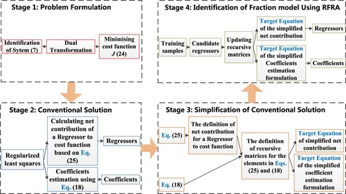18) ). Thirdly, recursive matrices are defined to derive a simplified and efficient computational framework for calculating the net contributions of model terms and the model coefficients. Finally, to identify the fraction model using RFRA, the elements of recursive matrices can be updated recursively without incurring much calculations. Substituting these recursive matrices into the target equations, the regressors are selected and the coefficients are estimated respectively. The schematic of the proposed RFRA is illustrated in Figure 2.

Figure 2. The schematic of the proposed RFRA method.

Suppose the model (2(2) $\mathit{y}=\mathit{a}\oslash \mathit{c}+\mathit{e}=\left({\mathit{P}}_n{\mathbf{\Theta }}_n\right)\oslash \left({\mathit{P}}_d{\mathbf{\Theta }}_d\right)+\mathit{e}$(2) ) has a maximum of $(m+1)/2$ regression terms both in the numerator and the denominator, the matrix of candidate regression terms for (2(2) $\mathit{y}=\mathit{a}\oslash \mathit{c}+\mathit{e}=\left({\mathit{P}}_n{\mathbf{\Theta }}_n\right)\oslash \left({\mathit{P}}_d{\mathbf{\Theta }}_d\right)+\mathit{e}$(2) ) can be initially set as ${\mathit{\Omega }}_{(m+1)/2}=[\mathbf{1},{\mathit{\omega }}_1,\dots ,{\mathit{\omega }}_{(m-1)/2}]$. Then the transformed linear model (7(7) $\mathit{Y}=\mathbf{\Phi }\mathbf{\Theta }+\mathit{c}\odot \mathit{e}=\mathbf{\Phi }\mathbf{\Theta }+\mathbf{\Xi }$(7) ) has a maximum of m regression terms because the constant term in the denominator should have been moved as a part of the output. The matrix of candidate regression terms in (7(7) $\mathit{Y}=\mathbf{\Phi }\mathbf{\Theta }+\mathit{c}\odot \mathit{e}=\mathbf{\Phi }\mathbf{\Theta }+\mathbf{\Xi }$(7) ) can be initially set as ${\mathit{Q}}_m=[{\mathit{\phi }}_1,\dots ,{\mathit{\phi }}_m]=[\mathbf{1},{\mathit{\omega }}_1,\dots ,{\mathit{\omega }}_{(m-1)/2},-\mathit{y}\odot {\mathit{\omega }}_1,\dots ,-\mathit{y}\odot {\mathit{\omega }}_{(m-1)/2}]$ and the corresponding auxiliary matrix for regularisation can be initially set as ${\mathit{{\rm Y}}}_m=[{\mathit{\kappa }}_1,\dots ,{\mathit{\kappa }}_m]=[\mathbf{0},\mathbf{0},\dots ,\mathbf{0},{\mathit{\omega }}_1,\dots ,{\mathit{\omega }}_{(m-1)/2}]$ respectively, where the indices of the elements in ${\mathit{Q}}_{m-k+1}$ and ${\mathit{{\rm Y}}}_{m-k+1}$ at the kth iteration start from k, and thus ${\mathit{\phi }}_i$ and ${\mathit{\kappa }}_i$ are the $(i-k+1)$th candidate terms in the candidate regression matrix ${\mathit{Q}}_{m-k+1}$ and the augmented matrix ${\mathit{{\rm Y}}}_{m-k+1}$, respectively.

After the kth regressors has been selected into the model (7(7) $\mathit{Y}=\mathbf{\Phi }\mathbf{\Theta }+\mathit{c}\odot \mathit{e}=\mathbf{\Phi }\mathbf{\Theta }+\mathbf{\Xi }$(7) ), the selected regression term matrix is recorded as ${\mathbf{\Phi }}_k=[{\mathit{\varphi }}_1,\dots ,{\mathit{\varphi }}_k]$ and the selected augmented term matrix is recorded as ${\mathbf{\Psi }}_k=[{\mathit{\psi }}_1,\dots ,{\mathit{\psi }}_k]$. Then the remaining candidate regressor matrix and the candidate augmented matrix are ${\mathit{Q}}_{m-k}=[{\mathit{\phi }}_{k+1},\dots ,{\mathit{\phi }}_m]$ and ${\mathit{{\rm Y}}}_{m-k}=[{\mathit{\kappa }}_{k+1},\dots ,{\mathit{\kappa }}_m]$ respectively. Thus the optimal model coefficients and the corresponding cost function are given as (26) $\begin{array}{rl}{\stackrel{\mathbf{ˆ}}{\mathbf{\Theta }}}_k& =({\mathbf{\Phi }}_k^{\mathrm{T}}{\mathbf{\Phi }}_k+\lambda {\mathbf{\Psi }}_k^{\mathrm{T}}{\mathbf{\Psi }}_k{)}^{-1}({\mathbf{\Phi }}_k^{\mathrm{T}}\mathit{Y}-\lambda {\mathbf{\Psi }}_k^{\mathrm{T}}\mathit{E})\end{array}$(26) (27) $\begin{array}{rl}{\mathit{J}}_k& ={\mathit{Y}}^{\mathrm{T}}(\mathit{I}-{\mathbf{\Phi }}_k({\mathbf{\Phi }}_k^{\mathrm{T}}{\mathbf{\Phi }}_k+\lambda {\mathbf{\Psi }}_k^{\mathrm{T}}{\mathbf{\Psi }}_k{)}^{-1}{\mathbf{\Phi }}_k^{\mathrm{T}})\mathit{Y}\\ & +2\lambda {\mathit{Y}}^{\mathrm{T}}{\mathbf{\Psi }}_k({\mathbf{\Phi }}_k^{\mathrm{T}}{\mathbf{\Phi }}_k+\lambda {\mathbf{\Psi }}_k^{\mathrm{T}}{\mathbf{\Psi }}_k{)}^{-1}{\mathbf{\Phi }}_k^{\mathrm{T}}\mathit{E}\\ & +\lambda {\mathit{E}}^{\mathrm{T}}(\mathit{I}-\lambda {\mathbf{\Psi }}_k({\mathbf{\Phi }}_k^{\mathrm{T}}{\mathbf{\Phi }}_k+\lambda {\mathbf{\Psi }}_k^{\mathrm{T}}{\mathbf{\Psi }}_k{)}^{-1}{\mathbf{\Psi }}_k^{\mathrm{T}})\mathit{E}\end{array}$(27) Before introducing the regularised fast recursive algorithm, a recursive matrix at the kth iteration is defined as (28) ${\mathit{M}}_k\triangleq {\mathbf{\Phi }}_k^{\mathrm{T}}{\mathbf{\Phi }}_k+\lambda {\mathbf{\Psi }}_k^{\mathrm{T}}{\mathbf{\Psi }}_k$(28) And the inversion of ${\mathit{M}}_k^{-1}=({\mathbf{\Phi }}_k^{\mathrm{T}}{\mathbf{\Phi }}_k+\lambda {\mathbf{\Psi }}_k^{\mathrm{T}}{\mathbf{\Psi }}_k{)}^{-1}$ can be computed as follows (29) $\begin{array}{rl}{\mathit{M}}_k^{-1}& ={\left[\begin{array}{cc}{\mathit{M}}_{k-1}& \begin{array}{c}{\mathbf{\Phi }}_{k-1}^{\mathrm{T}}{\mathit{\varphi }}_k\\ +\lambda {\mathbf{\Psi }}_{k-1}^{\mathrm{T}}{\mathit{\psi }}_k\end{array}\\ {\mathit{\varphi }}_k^{\mathrm{T}}{\mathbf{\Phi }}_{k-1}+\lambda {\mathit{\psi }}_k^{\mathrm{T}}{\mathbf{\Psi }}_{k-1}& {\mathit{\varphi }}_k^{\mathrm{T}}{\mathit{\varphi }}_k+\lambda {\mathit{\psi }}_k^{\mathrm{T}}{\mathit{\psi }}_k\end{array}\right]}^{-1}\\ & =\left[\begin{array}{cc}{\mathit{F}}_{k-1}& {\mathit{g}}_{k-1}\\ {\mathit{g}}_{k-1}^{\mathrm{T}}& {\mathit{f}}_{k-1}\end{array}\right]\end{array}$(29) where ${\mathbf{\Phi }}_{k-1}=[{\mathit{\varphi }}_1,\dots ,{\mathit{\varphi }}_{k-1}]$ and ${\mathbf{\Psi }}_{k-1}=[{\mathit{\psi }}_1,\dots ,{\mathit{\psi }}_{k-1}]$.

Given that ${\mathit{M}}_k\cdot {\mathit{M}}_k^{-1}=\mathit{I}$, then ${\mathit{F}}_{k-1}$, ${\mathit{g}}_{k-1}$ and ${\mathit{f}}_{k-1}$ can be calculated as follows (30) $\{\begin{array}{l}{\displaystyle {\mathit{F}}_{k-1}=[{\mathit{M}}_{k-1}-({\mathbf{\Phi }}_{k-1}^{\mathrm{T}}{\mathit{\varphi }}_k+\lambda {\mathbf{\Psi }}_{k-1}^{\mathrm{T}}{\mathit{\psi }}_k)}\\ ({\mathit{\varphi }}_k^{\mathrm{T}}{\mathbf{\Phi }}_{k-1}+\lambda {\mathit{\psi }}_k^{\mathrm{T}}{\mathbf{\Psi }}_{k-1})/({\mathit{\varphi }}_k^{\mathrm{T}}{\mathit{\varphi }}_k+\lambda {\mathit{\psi }}_k^{\mathrm{T}}{\mathit{\psi }}_k){]}^{-1}\\ {\displaystyle {\mathit{g}}_{k-1}=-{\mathit{F}}_{k-1}({\mathbf{\Phi }}_{k-1}^{\mathrm{T}}{\mathit{\varphi }}_k+\lambda {\mathbf{\Psi }}_{k-1}^{\mathrm{T}}{\mathit{\psi }}_k)}\\ /({\mathit{\varphi }}_k^{\mathrm{T}}{\mathit{\varphi }}_k+\lambda {\mathit{\psi }}_k^{\mathrm{T}}{\mathit{\psi }}_k)\\ {\displaystyle {\mathit{f}}_{k-1}=\frac{\begin{array}{c}({\mathit{\varphi }}_k^{\mathrm{T}}{\mathit{\varphi }}_k+\lambda {\mathit{\psi }}_k^{\mathrm{T}}{\mathit{\psi }}_k)\\ +({\mathit{\varphi }}_k^{\mathrm{T}}{\mathbf{\Phi }}_{k-1}+\lambda {\mathit{\psi }}_k^{\mathrm{T}}{\mathbf{\Psi }}_{k-1}){\mathit{F}}_{k-1}\\ ({\mathbf{\Phi }}_{k-1}^{\mathrm{T}}{\mathit{\varphi }}_k+\lambda {\mathbf{\Psi }}_{k-1}^{\mathrm{T}}{\mathit{\psi }}_k)\end{array}}{({\mathit{\varphi }}_k^{\mathrm{T}}{\mathit{\varphi }}_k+\lambda {\mathit{\psi }}_k^{\mathrm{T}}{\mathit{\psi }}_k{)}^2}}\end{array}$(30) According to the matrix inversion lemma $[\mathit{A}+\mathbf{\text{B}}\mathit{C}\mathit{D}{]}^{-1}={\mathit{A}}^{-1}-{\mathit{A}}^{-1}\mathit{B}[\mathit{D}{\mathit{A}}^{-1}\mathit{B}+{\mathit{C}}^{-1}{]}^{-1}\mathit{D}{\mathit{A}}^{-1}$, ${\mathit{F}}_{k-1}$ can be computed as follows (31) ${\mathit{F}}_{k-1}={\mathit{M}}_{k-1}^{-1}+\frac{\begin{array}{c}{\mathit{M}}_{k-1}^{-1}({\mathbf{\Phi }}_{k-1}^{\mathrm{T}}{\mathit{\varphi }}_k+\lambda {\mathbf{\Psi }}_{k-1}^{\mathrm{T}}{\mathit{\psi }}_k)\\ ({\mathit{\varphi }}_k^{\mathrm{T}}{\mathbf{\Phi }}_{k-1}+\lambda {\mathit{\psi }}_k^{\mathrm{T}}{\mathbf{\Psi }}_{k-1}){\mathit{M}}_{k-1}^{-1}\end{array}}{\begin{array}{c}{\mathit{\varphi }}_k^{\mathrm{T}}{\mathit{\varphi }}_k+\lambda {\mathit{\psi }}_k^{\mathrm{T}}{\mathit{\psi }}_k\\ -({\mathit{\varphi }}_k^{\mathrm{T}}{\mathbf{\Phi }}_{k-1}+\lambda {\mathit{\psi }}_k^{\mathrm{T}}{\mathbf{\Psi }}_{k-1}){\mathit{M}}_{k-1}^{-1}\\ ({\mathbf{\Phi }}_{k-1}^{\mathrm{T}}{\mathit{\varphi }}_k+\lambda {\mathbf{\Psi }}_{k-1}^{\mathrm{T}}{\mathit{\psi }}_k)\end{array}}$(31) Thus, after kth selection, the cost function of Equation (27(27) $\begin{array}{rl}{\mathit{J}}_k& ={\mathit{Y}}^{\mathrm{T}}(\mathit{I}-{\mathbf{\Phi }}_k({\mathbf{\Phi }}_k^{\mathrm{T}}{\mathbf{\Phi }}_k+\lambda {\mathbf{\Psi }}_k^{\mathrm{T}}{\mathbf{\Psi }}_k{)}^{-1}{\mathbf{\Phi }}_k^{\mathrm{T}})\mathit{Y}\\ & +2\lambda {\mathit{Y}}^{\mathrm{T}}{\mathbf{\Psi }}_k({\mathbf{\Phi }}_k^{\mathrm{T}}{\mathbf{\Phi }}_k+\lambda {\mathbf{\Psi }}_k^{\mathrm{T}}{\mathbf{\Psi }}_k{)}^{-1}{\mathbf{\Phi }}_k^{\mathrm{T}}\mathit{E}\\ & +\lambda {\mathit{E}}^{\mathrm{T}}(\mathit{I}-\lambda {\mathbf{\Psi }}_k({\mathbf{\Phi }}_k^{\mathrm{T}}{\mathbf{\Phi }}_k+\lambda {\mathbf{\Psi }}_k^{\mathrm{T}}{\mathbf{\Psi }}_k{)}^{-1}{\mathbf{\Psi }}_k^{\mathrm{T}})\mathit{E}\end{array}$(27) ) becomes (32) $\begin{array}{rl}{\mathit{J}}_k& ={\mathit{Y}}^{\mathrm{T}}(\mathit{I}-{\mathbf{\Phi }}_k{\mathit{M}}_k^{-1}{\mathbf{\Phi }}_k^{\mathrm{T}})\mathit{Y}+2\lambda {\mathit{Y}}^{\mathrm{T}}{\mathbf{\Phi }}_k{\mathit{M}}_k^{-1}{\mathbf{\Psi }}_k^{\mathrm{T}}\mathit{E}\\ & +\lambda {\mathit{E}}^{\mathrm{T}}(\mathit{I}-\lambda {\mathbf{\Psi }}_k{\mathit{M}}_k^{-1}{\mathbf{\Psi }}_k^{\mathrm{T}})\mathit{E}\end{array}$(32) Assuming the regression term ${\mathit{\phi }}_i$ is selected from the candidate matrix ${\mathit{Q}}_{m-k}$ at $(k+1)$th selection, the selected regression term matrix becomes ${\mathbf{\Phi }}_{k+1}=[{\mathbf{\Phi }}_k,{\mathit{\phi }}_i]$ and the selected augmented regression term matrix is ${\mathbf{\Psi }}_{k+1}=[{\mathbf{\Psi }}_k,{\mathit{\kappa }}_i]$, while the remaining candidate regressor matrix and the candidate augmented matrix are ${\mathit{Q}}_{m-k-1}=[{\mathit{\phi }}_{k+1},\dots ,{\mathit{\phi }}_{i-1},{\mathit{\phi }}_{i+1},\dots ,{\mathit{\phi }}_m]$ and ${\mathit{{\rm Y}}}_{m-k-1}=[{\mathit{\kappa }}_{k+1},\dots ,{\mathit{\kappa }}_{i-1},{\mathit{\kappa }}_{i+1},\dots ,{\mathit{\kappa }}_m]$ respectively.

Thus, the cost function is updated as follows (33) $\begin{array}{rl}{\mathit{J}}_{k+1}& ={\mathit{Y}}^{\mathrm{T}}(\mathit{I}-{\mathbf{\Phi }}_{k+1}{\mathit{M}}_{k+1}^{-1}{\mathbf{\Phi }}_{k+1}^{\mathrm{T}})\mathit{Y}\\ & +2\lambda {\mathit{Y}}^{\mathrm{T}}{\mathbf{\Phi }}_{k+1}{\mathit{M}}_{k+1}^{-1}{\mathbf{\Psi }}_{k+1}^{\mathrm{T}}\mathit{E}\\ & +\lambda {\mathit{E}}^{\mathrm{T}}(\mathit{I}-\lambda {\mathbf{\Psi }}_{k+1}{\mathit{M}}_{k+1}^{-1}{\mathbf{\Psi }}_{k+1}^{\mathrm{T}})\mathit{E}\end{array}$(33) where ${\mathit{M}}_{k+1}={\mathbf{\Phi }}_{k+1}^{\mathrm{T}}{\mathbf{\Phi }}_{k+1}+\lambda {\mathbf{\Psi }}_{k+1}^{\mathrm{T}}{\mathbf{\Psi }}_{k+1}$.

Then, the net contribution of the selected term (${\mathit{\phi }}_i$) is given as (34) $\delta {\mathit{J}}_{k+1}={\mathit{J}}_{k+1}-{\mathit{J}}_k$(34) In order to simplify the calculations, three recursive matrices (indexed with (1), (2) and (3)) at $(k+1)$th iteration, recorded as ${\mathit{R}}_{k+1}^{\left(1\right)}$, ${\mathit{R}}_{k+1}^{\left(2\right)}$ and ${\mathit{R}}_{k+1}^{\left(3\right)}$, are defined as (35) $\begin{array}{rl}{\mathit{R}}_{k+1}^{\left(1\right)}& \triangleq \mathit{I}-{\mathbf{\Phi }}_{k+1}{\mathit{M}}_{k+1}^{-1}{\mathbf{\Phi }}_{k+1}^{\mathrm{T}}\end{array}$(35) (36) $\begin{array}{rl}{\mathit{R}}_{k+1}^{\left(2\right)}& \triangleq \mathit{I}-\lambda {\mathbf{\Psi }}_{k+1}{\mathit{M}}_{k+1}^{-1}{\mathbf{\Psi }}_{k+1}^{\mathrm{T}}\end{array}$(36) (37) $\begin{array}{rl}{\mathit{R}}_{k+1}^{\left(3\right)}& \triangleq -{\mathbf{\Phi }}_{k+1}{\mathit{M}}_{k+1}^{-1}{\mathbf{\Psi }}_{k+1}^{\mathrm{T}}\end{array}$(37) where the matrix sizes of ${\mathit{R}}_{k+1}^{\left(1\right)}$, ${\mathit{R}}_{k+1}^{\left(2\right)}$ and ${\mathit{R}}_{k+1}^{\left(3\right)}$ are all N by N, and ${\mathit{R}}_0^{\left(1\right)}={\mathit{I}}_{N\times N}$, ${\mathit{R}}_0^{\left(2\right)}={\mathit{I}}_{N\times N}$, ${\mathit{R}}_0^{\left(3\right)}={\mathbf{0}}_{N\times N}$.

Having defined these three recursive matrices, the explicit formulation to efficiently calculate the net contribution can be derived first. According to the calculation of ${\mathit{M}}_k^{-1}$ using Equations (30(30) $\{\begin{array}{l}{\displaystyle {\mathit{F}}_{k-1}=[{\mathit{M}}_{k-1}-({\mathbf{\Phi }}_{k-1}^{\mathrm{T}}{\mathit{\varphi }}_k+\lambda {\mathbf{\Psi }}_{k-1}^{\mathrm{T}}{\mathit{\psi }}_k)}\\ ({\mathit{\varphi }}_k^{\mathrm{T}}{\mathbf{\Phi }}_{k-1}+\lambda {\mathit{\psi }}_k^{\mathrm{T}}{\mathbf{\Psi }}_{k-1})/({\mathit{\varphi }}_k^{\mathrm{T}}{\mathit{\varphi }}_k+\lambda {\mathit{\psi }}_k^{\mathrm{T}}{\mathit{\psi }}_k){]}^{-1}\\ {\displaystyle {\mathit{g}}_{k-1}=-{\mathit{F}}_{k-1}({\mathbf{\Phi }}_{k-1}^{\mathrm{T}}{\mathit{\varphi }}_k+\lambda {\mathbf{\Psi }}_{k-1}^{\mathrm{T}}{\mathit{\psi }}_k)}\\ /({\mathit{\varphi }}_k^{\mathrm{T}}{\mathit{\varphi }}_k+\lambda {\mathit{\psi }}_k^{\mathrm{T}}{\mathit{\psi }}_k)\\ {\displaystyle {\mathit{f}}_{k-1}=\frac{\begin{array}{c}({\mathit{\varphi }}_k^{\mathrm{T}}{\mathit{\varphi }}_k+\lambda {\mathit{\psi }}_k^{\mathrm{T}}{\mathit{\psi }}_k)\\ +({\mathit{\varphi }}_k^{\mathrm{T}}{\mathbf{\Phi }}_{k-1}+\lambda {\mathit{\psi }}_k^{\mathrm{T}}{\mathbf{\Psi }}_{k-1}){\mathit{F}}_{k-1}\\ ({\mathbf{\Phi }}_{k-1}^{\mathrm{T}}{\mathit{\varphi }}_k+\lambda {\mathbf{\Psi }}_{k-1}^{\mathrm{T}}{\mathit{\psi }}_k)\end{array}}{({\mathit{\varphi }}_k^{\mathrm{T}}{\mathit{\varphi }}_k+\lambda {\mathit{\psi }}_k^{\mathrm{T}}{\mathit{\psi }}_k{)}^2}}\end{array}$(30) ) and (31(31) ${\mathit{F}}_{k-1}={\mathit{M}}_{k-1}^{-1}+\frac{\begin{array}{c}{\mathit{M}}_{k-1}^{-1}({\mathbf{\Phi }}_{k-1}^{\mathrm{T}}{\mathit{\varphi }}_k+\lambda {\mathbf{\Psi }}_{k-1}^{\mathrm{T}}{\mathit{\psi }}_k)\\ ({\mathit{\varphi }}_k^{\mathrm{T}}{\mathbf{\Phi }}_{k-1}+\lambda {\mathit{\psi }}_k^{\mathrm{T}}{\mathbf{\Psi }}_{k-1}){\mathit{M}}_{k-1}^{-1}\end{array}}{\begin{array}{c}{\mathit{\varphi }}_k^{\mathrm{T}}{\mathit{\varphi }}_k+\lambda {\mathit{\psi }}_k^{\mathrm{T}}{\mathit{\psi }}_k\\ -({\mathit{\varphi }}_k^{\mathrm{T}}{\mathbf{\Phi }}_{k-1}+\lambda {\mathit{\psi }}_k^{\mathrm{T}}{\mathbf{\Psi }}_{k-1}){\mathit{M}}_{k-1}^{-1}\\ ({\mathbf{\Phi }}_{k-1}^{\mathrm{T}}{\mathit{\varphi }}_k+\lambda {\mathbf{\Psi }}_{k-1}^{\mathrm{T}}{\mathit{\psi }}_k)\end{array}}$(31) ), the recursive matrices defined in Equations (35(35) $\begin{array}{rl}{\mathit{R}}_{k+1}^{\left(1\right)}& \triangleq \mathit{I}-{\mathbf{\Phi }}_{k+1}{\mathit{M}}_{k+1}^{-1}{\mathbf{\Phi }}_{k+1}^{\mathrm{T}}\end{array}$(35) ), (36(36) $\begin{array}{rl}{\mathit{R}}_{k+1}^{\left(2\right)}& \triangleq \mathit{I}-\lambda {\mathbf{\Psi }}_{k+1}{\mathit{M}}_{k+1}^{-1}{\mathbf{\Psi }}_{k+1}^{\mathrm{T}}\end{array}$(36) ) and (37(37) $\begin{array}{rl}{\mathit{R}}_{k+1}^{\left(3\right)}& \triangleq -{\mathbf{\Phi }}_{k+1}{\mathit{M}}_{k+1}^{-1}{\mathbf{\Psi }}_{k+1}^{\mathrm{T}}\end{array}$(37) ) can be recursively updated as follows (38) $\begin{array}{rl}{\mathit{R}}_{k+1}^{\left(1\right)}& ={\mathit{R}}_k^{\left(1\right)}-\frac{\begin{array}{c}({\mathit{R}}_k^{\left(1\right)}{\mathit{\phi }}_i+\lambda {\mathit{R}}_k^{\left(3\right)}{\mathit{\kappa }}_i)({\mathit{\phi }}_i^{\mathrm{T}}\\ ({\mathit{R}}_k^{\left(1\right)}{)}^{\mathrm{T}}+\lambda {\mathit{\kappa }}_i^{\mathrm{T}}({\mathit{R}}_k^{\left(3\right)}{)}^{\mathrm{T}})\end{array}}{\begin{array}{c}({\mathit{\phi }}_i^{\mathrm{T}}{\mathit{R}}_k^{\left(1\right)}{\mathit{\phi }}_i+\lambda {\mathit{\kappa }}_i^{\mathrm{T}}{\mathit{R}}_k^{\left(2\right)}{\mathit{\kappa }}_i\\ +2\lambda {\mathit{\phi }}_i^{\mathrm{T}}{\mathit{R}}_k^{\left(3\right)}{\mathit{\kappa }}_i)\end{array}}\\ & \times k=0,\dots ,m-1,i=k+1,\dots ,m.\end{array}$(38) (39) $\begin{array}{rl}{\mathit{R}}_{k+1}^{\left(2\right)}& ={\mathit{R}}_k^{\left(2\right)}-\frac{\begin{array}{c}({\mathit{R}}_k^{\left(2\right)}{\mathit{\kappa }}_i+({\mathit{R}}_k^{\left(3\right)}{)}^{\mathrm{T}}{\mathit{\phi }}_i)\\ \left({\mathit{\kappa }}_i^{\mathrm{T}}\right({\mathit{R}}_k^{\left(2\right)}{)}^{\mathrm{T}}+{\mathit{\phi }}_i^{\mathrm{T}}{\mathit{R}}_k^{\left(3\right)})\end{array}}{\begin{array}{c}({\mathit{\phi }}_i^{\mathrm{T}}{\mathit{R}}_k^{\left(1\right)}{\mathit{\phi }}_i+\lambda {\mathit{\kappa }}_i^{\mathrm{T}}{\mathit{R}}_k^{\left(2\right)}{\mathit{\kappa }}_i\\ +2\lambda {\mathit{\phi }}_i^{\mathrm{T}}{\mathit{R}}_k^{\left(3\right)}{\mathit{\kappa }}_i)\end{array}}\\ & \times k=0,\dots ,m-1,i=k+1,\dots ,m.\end{array}$(39) (40) $\begin{array}{rl}{\mathit{R}}_{k+1}^{\left(3\right)}& ={\mathit{R}}_k^{\left(3\right)}-\frac{\begin{array}{c}({\mathit{R}}_k^{\left(1\right)}{\mathit{\phi }}_i+\lambda {\mathit{R}}_k^{\left(3\right)}{\mathit{\kappa }}_i)\\ \left({\mathit{\kappa }}_i^{\mathrm{T}}\right({\mathit{R}}_k^{\left(2\right)}{)}^{\mathrm{T}}+{\mathit{\phi }}_i^{\mathrm{T}}{\mathit{R}}_k^{\left(3\right)})\end{array}}{\begin{array}{c}({\mathit{\phi }}_i^{\mathrm{T}}{\mathit{R}}_k^{\left(1\right)}{\mathit{\phi }}_i+\lambda {\mathit{\kappa }}_i^{\mathrm{T}}{\mathit{R}}_k^{\left(2\right)}{\mathit{\kappa }}_i\\ +2\lambda {\mathit{\phi }}_i^{\mathrm{T}}{\mathit{R}}_k^{\left(3\right)}{\mathit{\kappa }}_i)\end{array}}\\ & \times k=0,\dots ,m-1,i=k+1,\dots ,m.\end{array}$(40) The proof of these properties in Equations (38(38) $\begin{array}{rl}{\mathit{R}}_{k+1}^{\left(1\right)}& ={\mathit{R}}_k^{\left(1\right)}-\frac{\begin{array}{c}({\mathit{R}}_k^{\left(1\right)}{\mathit{\phi }}_i+\lambda {\mathit{R}}_k^{\left(3\right)}{\mathit{\kappa }}_i)({\mathit{\phi }}_i^{\mathrm{T}}\\ ({\mathit{R}}_k^{\left(1\right)}{)}^{\mathrm{T}}+\lambda {\mathit{\kappa }}_i^{\mathrm{T}}({\mathit{R}}_k^{\left(3\right)}{)}^{\mathrm{T}})\end{array}}{\begin{array}{c}({\mathit{\phi }}_i^{\mathrm{T}}{\mathit{R}}_k^{\left(1\right)}{\mathit{\phi }}_i+\lambda {\mathit{\kappa }}_i^{\mathrm{T}}{\mathit{R}}_k^{\left(2\right)}{\mathit{\kappa }}_i\\ +2\lambda {\mathit{\phi }}_i^{\mathrm{T}}{\mathit{R}}_k^{\left(3\right)}{\mathit{\kappa }}_i)\end{array}}\\ & \times k=0,\dots ,m-1,i=k+1,\dots ,m.\end{array}$(38) )–(40(40) $\begin{array}{rl}{\mathit{R}}_{k+1}^{\left(3\right)}& ={\mathit{R}}_k^{\left(3\right)}-\frac{\begin{array}{c}({\mathit{R}}_k^{\left(1\right)}{\mathit{\phi }}_i+\lambda {\mathit{R}}_k^{\left(3\right)}{\mathit{\kappa }}_i)\\ \left({\mathit{\kappa }}_i^{\mathrm{T}}\right({\mathit{R}}_k^{\left(2\right)}{)}^{\mathrm{T}}+{\mathit{\phi }}_i^{\mathrm{T}}{\mathit{R}}_k^{\left(3\right)})\end{array}}{\begin{array}{c}({\mathit{\phi }}_i^{\mathrm{T}}{\mathit{R}}_k^{\left(1\right)}{\mathit{\phi }}_i+\lambda {\mathit{\kappa }}_i^{\mathrm{T}}{\mathit{R}}_k^{\left(2\right)}{\mathit{\kappa }}_i\\ +2\lambda {\mathit{\phi }}_i^{\mathrm{T}}{\mathit{R}}_k^{\left(3\right)}{\mathit{\kappa }}_i)\end{array}}\\ & \times k=0,\dots ,m-1,i=k+1,\dots ,m.\end{array}$(40) ) is given in Appendix 2.

In addition, based on the definitions in Equation (35(35) $\begin{array}{rl}{\mathit{R}}_{k+1}^{\left(1\right)}& \triangleq \mathit{I}-{\mathbf{\Phi }}_{k+1}{\mathit{M}}_{k+1}^{-1}{\mathbf{\Phi }}_{k+1}^{\mathrm{T}}\end{array}$(35) )–(37(37) $\begin{array}{rl}{\mathit{R}}_{k+1}^{\left(3\right)}& \triangleq -{\mathbf{\Phi }}_{k+1}{\mathit{M}}_{k+1}^{-1}{\mathbf{\Psi }}_{k+1}^{\mathrm{T}}\end{array}$(37) ), several properties can be inferred as given in Equations (41(41) $\begin{array}{rl}{\mathit{R}}_k^{\left(1\right)}& =({\mathit{R}}_k^{\left(1\right)}{)}^{\mathrm{T}};{\mathit{R}}_k^{\left(2\right)}=({\mathit{R}}_k^{\left(2\right)}{)}^{\mathrm{T}},\\ & k=0,1,\dots ,m-1.\end{array}$(41) )–(44(44) $\begin{array}{rl}{\mathit{R}}_k^{\left(3\right)}& ={\mathit{R}}_k^{\left(1\right)}{\mathit{R}}_k^{\left(3\right)}+{\mathit{R}}_k^{\left(3\right)}{\mathit{R}}_k^{\left(2\right)};k=0,1,\dots ,m-1.\end{array}$(44) ). (41) $\begin{array}{rl}{\mathit{R}}_k^{\left(1\right)}& =({\mathit{R}}_k^{\left(1\right)}{)}^{\mathrm{T}};{\mathit{R}}_k^{\left(2\right)}=({\mathit{R}}_k^{\left(2\right)}{)}^{\mathrm{T}},\\ & k=0,1,\dots ,m-1.\end{array}$(41) (42) $\begin{array}{rl}{\mathit{R}}_k^{\left(1\right)}& =({\mathit{R}}_k^{\left(1\right)}{)}^2+\lambda {\mathit{R}}_k^{\left(3\right)}({\mathit{R}}_k^{\left(3\right)}{)}^{\mathrm{T}};k=0,1,\dots ,m-1.\end{array}$(42) (43) $\begin{array}{rl}{\mathit{R}}_k^{\left(2\right)}& =({\mathit{R}}_k^{\left(2\right)}{)}^2+({\mathit{R}}_k^{\left(3\right)}{)}^{\mathrm{T}}{\mathit{R}}_k^{\left(3\right)};k=0,1,\dots ,m-1.\end{array}$(43) (44) $\begin{array}{rl}{\mathit{R}}_k^{\left(3\right)}& ={\mathit{R}}_k^{\left(1\right)}{\mathit{R}}_k^{\left(3\right)}+{\mathit{R}}_k^{\left(3\right)}{\mathit{R}}_k^{\left(2\right)};k=0,1,\dots ,m-1.\end{array}$(44) Then, the cost function ${\mathit{J}}_k$ at the kth iteration can be reformulated as (45) $\begin{array}{rl}{\mathit{J}}_k& ={\mathit{Y}}^{\mathrm{T}}{\mathit{R}}_k^{\left(1\right)}\mathit{Y}+\lambda {\mathit{E}}^{\mathrm{T}}{\mathit{R}}_k^{\left(2\right)}\mathit{E}+2\lambda {\mathit{Y}}^{\mathrm{T}}{\mathit{R}}_k^{\left(3\right)}\mathit{E}+\lambda {\mathit{E}}^{\mathrm{T}}\mathit{E}\\ & k=0,\dots ,m-1.\end{array}$(45) And, the net contribution of the selected term (${\mathit{\phi }}_i$) in Equation (34(34) $\delta {\mathit{J}}_{k+1}={\mathit{J}}_{k+1}-{\mathit{J}}_k$(34) ) can be rewritten as (46) $\begin{array}{rl}\delta {\mathit{J}}_{k+1}\left({\mathit{\phi }}_i\right)& ={\mathit{Y}}^{\mathrm{T}}({\mathit{R}}_{k+1}^{\left(1\right)}-{\mathit{R}}_k^{\left(1\right)})\mathit{Y}\\ & +\lambda {\mathit{E}}^{\mathrm{T}}({\mathit{R}}_{k+1}^{\left(2\right)}-{\mathit{R}}_k^{\left(2\right)})\mathit{E}\\ & +2\lambda {\mathit{Y}}^{\mathrm{T}}({\mathit{R}}_{k+1}^{\left(3\right)}-{\mathit{R}}_k^{\left(3\right)})\mathit{E}\\ & +(\lambda {\mathit{E}}^{\mathrm{T}}\mathit{E}-\lambda {\mathit{E}}^{\mathrm{T}}\mathit{E})\\ & ={\mathit{Y}}^{\mathrm{T}}({\mathit{R}}_{k+1}^{\left(1\right)}-{\mathit{R}}_k^{\left(1\right)})\mathit{Y}\\ & +\lambda {\mathit{E}}^{\mathrm{T}}({\mathit{R}}_{k+1}^{\left(2\right)}-{\mathit{R}}_k^{\left(2\right)})\mathit{E}\\ & +2\lambda {\mathit{Y}}^{\mathrm{T}}({\mathit{R}}_{k+1}^{\left(3\right)}-{\mathit{R}}_k^{\left(3\right)})\mathit{E}\\ & \times k=0,\dots ,m-1.\end{array}$(46) According to the properties given in Equations (38(38) $\begin{array}{rl}{\mathit{R}}_{k+1}^{\left(1\right)}& ={\mathit{R}}_k^{\left(1\right)}-\frac{\begin{array}{c}({\mathit{R}}_k^{\left(1\right)}{\mathit{\phi }}_i+\lambda {\mathit{R}}_k^{\left(3\right)}{\mathit{\kappa }}_i)({\mathit{\phi }}_i^{\mathrm{T}}\\ ({\mathit{R}}_k^{\left(1\right)}{)}^{\mathrm{T}}+\lambda {\mathit{\kappa }}_i^{\mathrm{T}}({\mathit{R}}_k^{\left(3\right)}{)}^{\mathrm{T}})\end{array}}{\begin{array}{c}({\mathit{\phi }}_i^{\mathrm{T}}{\mathit{R}}_k^{\left(1\right)}{\mathit{\phi }}_i+\lambda {\mathit{\kappa }}_i^{\mathrm{T}}{\mathit{R}}_k^{\left(2\right)}{\mathit{\kappa }}_i\\ +2\lambda {\mathit{\phi }}_i^{\mathrm{T}}{\mathit{R}}_k^{\left(3\right)}{\mathit{\kappa }}_i)\end{array}}\\ & \times k=0,\dots ,m-1,i=k+1,\dots ,m.\end{array}$(38) )–(39(39) $\begin{array}{rl}{\mathit{R}}_{k+1}^{\left(2\right)}& ={\mathit{R}}_k^{\left(2\right)}-\frac{\begin{array}{c}({\mathit{R}}_k^{\left(2\right)}{\mathit{\kappa }}_i+({\mathit{R}}_k^{\left(3\right)}{)}^{\mathrm{T}}{\mathit{\phi }}_i)\\ \left({\mathit{\kappa }}_i^{\mathrm{T}}\right({\mathit{R}}_k^{\left(2\right)}{)}^{\mathrm{T}}+{\mathit{\phi }}_i^{\mathrm{T}}{\mathit{R}}_k^{\left(3\right)})\end{array}}{\begin{array}{c}({\mathit{\phi }}_i^{\mathrm{T}}{\mathit{R}}_k^{\left(1\right)}{\mathit{\phi }}_i+\lambda {\mathit{\kappa }}_i^{\mathrm{T}}{\mathit{R}}_k^{\left(2\right)}{\mathit{\kappa }}_i\\ +2\lambda {\mathit{\phi }}_i^{\mathrm{T}}{\mathit{R}}_k^{\left(3\right)}{\mathit{\kappa }}_i)\end{array}}\\ & \times k=0,\dots ,m-1,i=k+1,\dots ,m.\end{array}$(39) ), Equation (46(46) $\begin{array}{rl}\delta {\mathit{J}}_{k+1}\left({\mathit{\phi }}_i\right)& ={\mathit{Y}}^{\mathrm{T}}({\mathit{R}}_{k+1}^{\left(1\right)}-{\mathit{R}}_k^{\left(1\right)})\mathit{Y}\\ & +\lambda {\mathit{E}}^{\mathrm{T}}({\mathit{R}}_{k+1}^{\left(2\right)}-{\mathit{R}}_k^{\left(2\right)})\mathit{E}\\ & +2\lambda {\mathit{Y}}^{\mathrm{T}}({\mathit{R}}_{k+1}^{\left(3\right)}-{\mathit{R}}_k^{\left(3\right)})\mathit{E}\\ & +(\lambda {\mathit{E}}^{\mathrm{T}}\mathit{E}-\lambda {\mathit{E}}^{\mathrm{T}}\mathit{E})\\ & ={\mathit{Y}}^{\mathrm{T}}({\mathit{R}}_{k+1}^{\left(1\right)}-{\mathit{R}}_k^{\left(1\right)})\mathit{Y}\\ & +\lambda {\mathit{E}}^{\mathrm{T}}({\mathit{R}}_{k+1}^{\left(2\right)}-{\mathit{R}}_k^{\left(2\right)})\mathit{E}\\ & +2\lambda {\mathit{Y}}^{\mathrm{T}}({\mathit{R}}_{k+1}^{\left(3\right)}-{\mathit{R}}_k^{\left(3\right)})\mathit{E}\\ & \times k=0,\dots ,m-1.\end{array}$(46) ) can be calculated as follows (47) $\begin{array}{rl}\delta {\mathit{J}}_{k+1}\left({\mathit{\phi }}_i\right)& =-\frac{\begin{array}{c}{\mathit{Y}}^{\mathrm{T}}({\mathit{R}}_k^{\left(1\right)}{\mathit{\phi }}_i+\lambda {\mathit{R}}_k^{\left(3\right)}{\mathit{\kappa }}_i)\\ \left({\mathit{\phi }}_i^{\mathrm{T}}\right({\mathit{R}}_k^{\left(1\right)}{)}^{\mathrm{T}}+\lambda {\mathit{\kappa }}_i^{\mathrm{T}}\left({\mathit{R}}_k^{\left(3\right)}{)}^{\mathrm{T}}\right)\mathit{Y}\end{array}}{\begin{array}{c}({\mathit{\phi }}_i^{\mathrm{T}}{\mathit{R}}_k^{\left(1\right)}{\mathit{\phi }}_i+\lambda {\mathit{\kappa }}_i^{\mathrm{T}}{\mathit{R}}_k^{\left(2\right)}{\mathit{\kappa }}_i\\ +2\lambda {\mathit{\phi }}_i^{\mathrm{T}}{\mathit{R}}_k^{\left(3\right)}{\mathit{\kappa }}_i)\end{array}}\\ & -\lambda \frac{\begin{array}{c}{\mathit{E}}^{\mathrm{T}}({\mathit{R}}_k^{\left(2\right)}{\mathit{\kappa }}_i+({\mathit{R}}_k^{\left(3\right)}{)}^{\mathrm{T}}{\mathit{\phi }}_i)\\ \left({\mathit{\kappa }}_i^{\mathrm{T}}\right({\mathit{R}}_k^{\left(2\right)}{)}^{\mathrm{T}}+{\mathit{\phi }}_i^{\mathrm{T}}{\mathit{R}}_k^{\left(3\right)})\mathit{E}\end{array}}{\begin{array}{c}({\mathit{\phi }}_i^{\mathrm{T}}{\mathit{R}}_k^{\left(1\right)}{\mathit{\phi }}_i+\lambda {\mathit{\kappa }}_i^{\mathrm{T}}{\mathit{R}}_k^{\left(2\right)}{\mathit{\kappa }}_i\\ +2\lambda {\mathit{\phi }}_i^{\mathrm{T}}{\mathit{R}}_k^{\left(3\right)}{\mathit{\kappa }}_i)\end{array}}\\ & -2\lambda \frac{\begin{array}{c}{\mathit{Y}}^{\mathrm{T}}({\mathit{R}}_k^{\left(1\right)}{\mathit{\phi }}_i+\lambda {\mathit{R}}_k^{\left(3\right)}{\mathit{\kappa }}_i)({\mathit{\kappa }}_i^{\mathrm{T}}\\ ({\mathit{R}}_k^{\left(2\right)}{)}^{\mathrm{T}}+{\mathit{\phi }}_i^{\mathrm{T}}{\mathit{R}}_k^{\left(3\right)})\mathit{E}\end{array}}{\begin{array}{c}({\mathit{\phi }}_i^{\mathrm{T}}{\mathit{R}}_k^{\left(1\right)}{\mathit{\phi }}_i+\lambda {\mathit{\kappa }}_i^{\mathrm{T}}{\mathit{R}}_k^{\left(2\right)}{\mathit{\kappa }}_i\\ +2\lambda {\mathit{\phi }}_i^{\mathrm{T}}{\mathit{R}}_k^{\left(3\right)}{\mathit{\kappa }}_i)\end{array}}\\ & \times k=0,\dots ,m-1.\end{array}$(47)

4.1.2. Fast computation of net contributions of model terms to the cost function

Note that there are m−k candidate terms (i.e. $i=k+1,\dots ,m$) to be evaluated at the $(k+1)$th iteration, and in order to select a new term ${\mathit{\varphi }}_{k+1}$ in ${\mathbf{\Phi }}_{k+1}$ to be included into the model, one needs to calculate $\delta {\mathit{J}}_{k+1}\left({\phi }_i\right)$ ($i=k+1,\dots ,m$) using (47(47) $\begin{array}{rl}\delta {\mathit{J}}_{k+1}\left({\mathit{\phi }}_i\right)& =-\frac{\begin{array}{c}{\mathit{Y}}^{\mathrm{T}}({\mathit{R}}_k^{\left(1\right)}{\mathit{\phi }}_i+\lambda {\mathit{R}}_k^{\left(3\right)}{\mathit{\kappa }}_i)\\ \left({\mathit{\phi }}_i^{\mathrm{T}}\right({\mathit{R}}_k^{\left(1\right)}{)}^{\mathrm{T}}+\lambda {\mathit{\kappa }}_i^{\mathrm{T}}\left({\mathit{R}}_k^{\left(3\right)}{)}^{\mathrm{T}}\right)\mathit{Y}\end{array}}{\begin{array}{c}({\mathit{\phi }}_i^{\mathrm{T}}{\mathit{R}}_k^{\left(1\right)}{\mathit{\phi }}_i+\lambda {\mathit{\kappa }}_i^{\mathrm{T}}{\mathit{R}}_k^{\left(2\right)}{\mathit{\kappa }}_i\\ +2\lambda {\mathit{\phi }}_i^{\mathrm{T}}{\mathit{R}}_k^{\left(3\right)}{\mathit{\kappa }}_i)\end{array}}\\ & -\lambda \frac{\begin{array}{c}{\mathit{E}}^{\mathrm{T}}({\mathit{R}}_k^{\left(2\right)}{\mathit{\kappa }}_i+({\mathit{R}}_k^{\left(3\right)}{)}^{\mathrm{T}}{\mathit{\phi }}_i)\\ \left({\mathit{\kappa }}_i^{\mathrm{T}}\right({\mathit{R}}_k^{\left(2\right)}{)}^{\mathrm{T}}+{\mathit{\phi }}_i^{\mathrm{T}}{\mathit{R}}_k^{\left(3\right)})\mathit{E}\end{array}}{\begin{array}{c}({\mathit{\phi }}_i^{\mathrm{T}}{\mathit{R}}_k^{\left(1\right)}{\mathit{\phi }}_i+\lambda {\mathit{\kappa }}_i^{\mathrm{T}}{\mathit{R}}_k^{\left(2\right)}{\mathit{\kappa }}_i\\ +2\lambda {\mathit{\phi }}_i^{\mathrm{T}}{\mathit{R}}_k^{\left(3\right)}{\mathit{\kappa }}_i)\end{array}}\\ & -2\lambda \frac{\begin{array}{c}{\mathit{Y}}^{\mathrm{T}}({\mathit{R}}_k^{\left(1\right)}{\mathit{\phi }}_i+\lambda {\mathit{R}}_k^{\left(3\right)}{\mathit{\kappa }}_i)({\mathit{\kappa }}_i^{\mathrm{T}}\\ ({\mathit{R}}_k^{\left(2\right)}{)}^{\mathrm{T}}+{\mathit{\phi }}_i^{\mathrm{T}}{\mathit{R}}_k^{\left(3\right)})\mathit{E}\end{array}}{\begin{array}{c}({\mathit{\phi }}_i^{\mathrm{T}}{\mathit{R}}_k^{\left(1\right)}{\mathit{\phi }}_i+\lambda {\mathit{\kappa }}_i^{\mathrm{T}}{\mathit{R}}_k^{\left(2\right)}{\mathit{\kappa }}_i\\ +2\lambda {\mathit{\phi }}_i^{\mathrm{T}}{\mathit{R}}_k^{\left(3\right)}{\mathit{\kappa }}_i)\end{array}}\\ & \times k=0,\dots ,m-1.\end{array}$(47) ) and the candidate term which is selected as ${\mathit{\varphi }}_{k+1}$ for inclusion into the model must have the maximal net contribution to the cost function, i.e. (48) $\mathrm{\Delta }{\mathit{J}}_{k+1}\left({\varphi }_{k+1}\right)=\underset{{\mathit{Q}}_{m-k}}{max}\mathrm{\Delta }{\mathit{J}}_{k+1}\left({\phi }_i\right)$(48) However, calculating the net contribution of m−k candidate terms using (47(47) $\begin{array}{rl}\delta {\mathit{J}}_{k+1}\left({\mathit{\phi }}_i\right)& =-\frac{\begin{array}{c}{\mathit{Y}}^{\mathrm{T}}({\mathit{R}}_k^{\left(1\right)}{\mathit{\phi }}_i+\lambda {\mathit{R}}_k^{\left(3\right)}{\mathit{\kappa }}_i)\\ \left({\mathit{\phi }}_i^{\mathrm{T}}\right({\mathit{R}}_k^{\left(1\right)}{)}^{\mathrm{T}}+\lambda {\mathit{\kappa }}_i^{\mathrm{T}}\left({\mathit{R}}_k^{\left(3\right)}{)}^{\mathrm{T}}\right)\mathit{Y}\end{array}}{\begin{array}{c}({\mathit{\phi }}_i^{\mathrm{T}}{\mathit{R}}_k^{\left(1\right)}{\mathit{\phi }}_i+\lambda {\mathit{\kappa }}_i^{\mathrm{T}}{\mathit{R}}_k^{\left(2\right)}{\mathit{\kappa }}_i\\ +2\lambda {\mathit{\phi }}_i^{\mathrm{T}}{\mathit{R}}_k^{\left(3\right)}{\mathit{\kappa }}_i)\end{array}}\\ & -\lambda \frac{\begin{array}{c}{\mathit{E}}^{\mathrm{T}}({\mathit{R}}_k^{\left(2\right)}{\mathit{\kappa }}_i+({\mathit{R}}_k^{\left(3\right)}{)}^{\mathrm{T}}{\mathit{\phi }}_i)\\ \left({\mathit{\kappa }}_i^{\mathrm{T}}\right({\mathit{R}}_k^{\left(2\right)}{)}^{\mathrm{T}}+{\mathit{\phi }}_i^{\mathrm{T}}{\mathit{R}}_k^{\left(3\right)})\mathit{E}\end{array}}{\begin{array}{c}({\mathit{\phi }}_i^{\mathrm{T}}{\mathit{R}}_k^{\left(1\right)}{\mathit{\phi }}_i+\lambda {\mathit{\kappa }}_i^{\mathrm{T}}{\mathit{R}}_k^{\left(2\right)}{\mathit{\kappa }}_i\\ +2\lambda {\mathit{\phi }}_i^{\mathrm{T}}{\mathit{R}}_k^{\left(3\right)}{\mathit{\kappa }}_i)\end{array}}\\ & -2\lambda \frac{\begin{array}{c}{\mathit{Y}}^{\mathrm{T}}({\mathit{R}}_k^{\left(1\right)}{\mathit{\phi }}_i+\lambda {\mathit{R}}_k^{\left(3\right)}{\mathit{\kappa }}_i)({\mathit{\kappa }}_i^{\mathrm{T}}\\ ({\mathit{R}}_k^{\left(2\right)}{)}^{\mathrm{T}}+{\mathit{\phi }}_i^{\mathrm{T}}{\mathit{R}}_k^{\left(3\right)})\mathit{E}\end{array}}{\begin{array}{c}({\mathit{\phi }}_i^{\mathrm{T}}{\mathit{R}}_k^{\left(1\right)}{\mathit{\phi }}_i+\lambda {\mathit{\kappa }}_i^{\mathrm{T}}{\mathit{R}}_k^{\left(2\right)}{\mathit{\kappa }}_i\\ +2\lambda {\mathit{\phi }}_i^{\mathrm{T}}{\mathit{R}}_k^{\left(3\right)}{\mathit{\kappa }}_i)\end{array}}\\ & \times k=0,\dots ,m-1.\end{array}$(47) ) will consume a large amount of computing resources including memory and time, to further simplify the calculations, a few intermediate matrices ${\mathit{A}}^{\left(l\right)}\triangleq \left[a_{j,i}^{\left(l\right)}\right]\in {\mathrm{\Re }}^{m\times m}$, ${\mathit{b}}^{\left(l\right)}\triangleq \left[b_i^{\left(l\right)}\right]\in {\mathrm{\Re }}^{1\times m}$ (l = 1, 2, 3, 4) are further introduced to calculate the net contribution to the cost function of the remaining m−k candidates. For ${\mathit{A}}^{\left(l\right)}$, the elements $a_{j,i}^{\left(l\right)}$ are given by: (49) $\begin{array}{rl}{a}_{j,i}^{\left(1\right)}& \triangleq \{\begin{array}{ll}0,& j>i\\ {\mathit{\varphi }}_j^T\left({\mathit{R}}_{j-1}^{\left(1\right)}\right){\mathit{\varphi }}_i,& j\le i\le k\\ {\mathit{\varphi }}_j^{\mathrm{T}}\left({\mathit{R}}_{j-1}^{\left(1\right)}\right){\mathit{\phi }}_i& j\le k,i=k+1,\dots ,m\\ {\mathit{\phi }}_j^{\mathrm{T}}\left({\mathit{R}}_k^{\left(1\right)}\right){\mathit{\phi }}_i& \begin{array}{l}j=k+1,\dots ,m,\\ i=j,\dots ,m\end{array}\end{array}\end{array}$(49) (50) $\begin{array}{rl}{a}_{j,i}^{\left(2\right)}& \triangleq \{\begin{array}{ll}0,& j>i\\ {\mathit{\psi }}_j^T\left({\mathit{R}}_{j-1}^{\left(2\right)}\right){\mathit{\psi }}_i,& j\le i\le k\\ {\mathit{\psi }}_j^T\left({\mathit{R}}_{j-1}^{\left(2\right)}\right){\mathit{\kappa }}_i,& j\le k,i=k+1,\dots ,m\\ {\mathit{\kappa }}_j^{\mathrm{T}}\left({\mathit{R}}_k^{\left(2\right)}\right){\mathit{\kappa }}_i& \begin{array}{l}j=k+1,\dots ,m,\\ i=j,\dots ,m\end{array}\end{array}\end{array}$(50) (51) $\begin{array}{rl}{a}_{j,i}^{\left(3\right)}& \triangleq \{\begin{array}{ll}0,& j>i\\ {\mathit{\psi }}_j^T\left({\mathit{R}}_{j-1}^{\left(3\right)}\right){\mathit{\varphi }}_i,& j\le i\le k\\ {\mathit{\psi }}_j^T\left({\mathit{R}}_{j-1}^{\left(3\right)}\right){\mathit{\phi }}_i,& j\le k,i=k+1,\dots ,m\\ {\mathit{\kappa }}_j^{\mathrm{T}}({\mathit{R}}_k^{\left(3\right)}{)}^{\mathrm{T}}{\mathit{\phi }}_i& \begin{array}{l}j=k+1,\dots ,m,\\ i=j,\dots ,m\end{array}\end{array}\end{array}$(51) (52) $\begin{array}{rl}{a}_{j,i}^{\left(4\right)}& \triangleq \{\begin{array}{ll}0,& j>i\\ {\mathit{\varphi }}_j^T\left({\mathit{R}}_{j-1}^{\left(3\right)}\right){\mathit{\psi }}_i,& j\le i\le k\\ {\mathit{\varphi }}_j^T\left({\mathit{R}}_{j-1}^{\left(3\right)}\right){\mathit{\kappa }}_i,& j\le k,i=k+1,\dots ,m\\ {\mathit{\phi }}_j^{\mathrm{T}}\left({\mathit{R}}_k^{\left(3\right)}\right){\mathit{\kappa }}_i& \begin{array}{l}j=k+1,\dots ,m,\\ i=j,\dots ,m\end{array}\end{array}\end{array}$(52) where the first three terms in each equation are used for recursive update of the elements, while the last term in each equation is used to calculate the net contribution of a candidate term and only the diagonal elements are used.

For ${\mathit{b}}^{\left(l\right)}$, the elements $b_i^{\left(l\right)}$ for the remaining candidates at $(k+1)$th iteration are given by: (53) $\begin{array}{rl}{b}_i^{\left(1\right)}& \triangleq \{\begin{array}{ll}{\mathit{Y}}^{\mathrm{T}}\left({\mathit{R}}_{i-1}^{\left(1\right)}\right){\mathit{\varphi }}_i& i\le k\\ {\mathit{Y}}^{\mathrm{T}}\left({\mathit{R}}_k^{\left(1\right)}\right){\mathit{\phi }}_i& i=k+1,\dots ,m\end{array}\end{array}$(53) (54) $\begin{array}{rl}{b}_i^{\left(3\right)}& \triangleq \{\begin{array}{ll}{\mathit{Y}}^{\mathrm{T}}\left({\mathit{R}}_{i-1}^{\left(3\right)}\right){\mathit{\psi }}_i& i\le k\\ {\mathit{Y}}^{\mathrm{T}}\left({\mathit{R}}_k^{\left(3\right)}\right){\mathit{\kappa }}_i& i=k+1,\dots ,m\end{array}\end{array}$(54) (55) $\begin{array}{rl}{b}_i^{\left(2\right)}& \triangleq \{\begin{array}{ll}{\mathit{E}}^{\mathrm{T}}\left({\mathit{R}}_{i-1}^{\left(2\right)}\right){\mathit{\psi }}_i& i\le k\\ {\mathit{E}}^{\mathrm{T}}\left({\mathit{R}}_k^{\left(2\right)}\right){\mathit{\kappa }}_i& i=k+1,\dots ,m\end{array}\end{array}$(55) (56) $\begin{array}{rl}{b}_i^{\left(4\right)}& \triangleq \{\begin{array}{ll}{\mathit{E}}^{\mathrm{T}}({\mathit{R}}_{i-1}^{\left(3\right)}{)}^{\mathrm{T}}{\mathit{\varphi }}_i& i\le k\\ {\mathit{E}}^{\mathrm{T}}({\mathit{R}}_k^{\left(3\right)}{)}^{\mathrm{T}}{\mathit{\phi }}_i& i=k+1,\dots ,m\end{array}\end{array}$(56) where the first term in each equation is used for recursive update of the elements, while the last term in each equation is used to calculate the net contribution.

Because of the symmetrical property and the properties in Equations (41(41) $\begin{array}{rl}{\mathit{R}}_k^{\left(1\right)}& =({\mathit{R}}_k^{\left(1\right)}{)}^{\mathrm{T}};{\mathit{R}}_k^{\left(2\right)}=({\mathit{R}}_k^{\left(2\right)}{)}^{\mathrm{T}},\\ & k=0,1,\dots ,m-1.\end{array}$(41) )–(44(44) $\begin{array}{rl}{\mathit{R}}_k^{\left(3\right)}& ={\mathit{R}}_k^{\left(1\right)}{\mathit{R}}_k^{\left(3\right)}+{\mathit{R}}_k^{\left(3\right)}{\mathit{R}}_k^{\left(2\right)};k=0,1,\dots ,m-1.\end{array}$(44) ), it is evident that $a_{j,i}^{\left(1\right)}=(a_{j,i}^{\left(1\right)}{)}^{\mathrm{T}}$, $a_{j,i}^{\left(2\right)}=(a_{j,i}^{\left(2\right)}{)}^{\mathrm{T}}$, $b_i^{\left(1\right)}=(b_i^{\left(1\right)}{)}^{\mathrm{T}}$ and $b_i^{\left(3\right)}=(b_i^{\left(3\right)}{)}^{\mathrm{T}}$.

Using Equation (38(38) $\begin{array}{rl}{\mathit{R}}_{k+1}^{\left(1\right)}& ={\mathit{R}}_k^{\left(1\right)}-\frac{\begin{array}{c}({\mathit{R}}_k^{\left(1\right)}{\mathit{\phi }}_i+\lambda {\mathit{R}}_k^{\left(3\right)}{\mathit{\kappa }}_i)({\mathit{\phi }}_i^{\mathrm{T}}\\ ({\mathit{R}}_k^{\left(1\right)}{)}^{\mathrm{T}}+\lambda {\mathit{\kappa }}_i^{\mathrm{T}}({\mathit{R}}_k^{\left(3\right)}{)}^{\mathrm{T}})\end{array}}{\begin{array}{c}({\mathit{\phi }}_i^{\mathrm{T}}{\mathit{R}}_k^{\left(1\right)}{\mathit{\phi }}_i+\lambda {\mathit{\kappa }}_i^{\mathrm{T}}{\mathit{R}}_k^{\left(2\right)}{\mathit{\kappa }}_i\\ +2\lambda {\mathit{\phi }}_i^{\mathrm{T}}{\mathit{R}}_k^{\left(3\right)}{\mathit{\kappa }}_i)\end{array}}\\ & \times k=0,\dots ,m-1,i=k+1,\dots ,m.\end{array}$(38) ) and the definition of $a_{j,i}^{\left(1\right)}$ in Equation (49(49) $\begin{array}{rl}{a}_{j,i}^{\left(1\right)}& \triangleq \{\begin{array}{ll}0,& j>i\\ {\mathit{\varphi }}_j^T\left({\mathit{R}}_{j-1}^{\left(1\right)}\right){\mathit{\varphi }}_i,& j\le i\le k\\ {\mathit{\varphi }}_j^{\mathrm{T}}\left({\mathit{R}}_{j-1}^{\left(1\right)}\right){\mathit{\phi }}_i& j\le k,i=k+1,\dots ,m\\ {\mathit{\phi }}_j^{\mathrm{T}}\left({\mathit{R}}_k^{\left(1\right)}\right){\mathit{\phi }}_i& \begin{array}{l}j=k+1,\dots ,m,\\ i=j,\dots ,m\end{array}\end{array}\end{array}$(49) ), $a_{j,i}^{\left(1\right)}$ can be recursively computed. Taking the second term of (49(49) $\begin{array}{rl}{a}_{j,i}^{\left(1\right)}& \triangleq \{\begin{array}{ll}0,& j>i\\ {\mathit{\varphi }}_j^T\left({\mathit{R}}_{j-1}^{\left(1\right)}\right){\mathit{\varphi }}_i,& j\le i\le k\\ {\mathit{\varphi }}_j^{\mathrm{T}}\left({\mathit{R}}_{j-1}^{\left(1\right)}\right){\mathit{\phi }}_i& j\le k,i=k+1,\dots ,m\\ {\mathit{\phi }}_j^{\mathrm{T}}\left({\mathit{R}}_k^{\left(1\right)}\right){\mathit{\phi }}_i& \begin{array}{l}j=k+1,\dots ,m,\\ i=j,\dots ,m\end{array}\end{array}\end{array}$(49) ) as an example, it can be recursively updated as follows (57) $\begin{array}{rl}{a}_{j,i}^{\left(1\right)}& ={\mathit{\varphi }}_j^{\mathrm{T}}\left({\mathit{R}}_{j-1}^{\left(1\right)}\right){\mathit{\varphi }}_i={\mathit{\varphi }}_j^{\mathrm{T}}{\mathit{R}}_{j-2}^{\left(1\right)}{\mathit{\varphi }}_i\\ & -\frac{\begin{array}{c}{\mathit{\varphi }}_j^{\mathrm{T}}({\mathit{R}}_{j-2}^{\left(1\right)}{\mathit{\varphi }}_{j-1}+\lambda {\mathit{R}}_{j-2}^{\left(3\right)}{\mathit{\psi }}_{j-1})\\ \left({\mathit{\varphi }}_{j-1}^{\mathrm{T}}\right({\mathit{R}}_{j-2}^{\left(1\right)}{)}^{\mathrm{T}}+\lambda {\mathit{\psi }}_{j-1}^{\mathrm{T}}\left({\mathit{R}}_{j-2}^{\left(3\right)}{)}^{\mathrm{T}}\right){\mathit{\varphi }}_i\end{array}}{\begin{array}{c}({\mathit{\varphi }}_{j-1}^{\mathrm{T}}{\mathit{R}}_{j-2}^{\left(1\right)}{\mathit{\varphi }}_{j-1}+\lambda {\mathit{\psi }}_{j-1}^{\mathrm{T}}{\mathit{R}}_{j-2}^{\left(2\right)}{\mathit{\psi }}_{j-1}\\ +2\lambda {\mathit{\varphi }}_{j-1}^{\mathrm{T}}{\mathit{R}}_{j-2}^{\left(3\right)}{\mathit{\psi }}_{j-1})\end{array}}\\ & ={\mathit{\varphi }}_j^{\mathrm{T}}{\mathit{R}}_{j-2}^{\left(1\right)}{\mathit{\varphi }}_i-\frac{(a_{j-1,j}^{\left(1\right)}+\lambda a_{j-1,j}^{\left(3\right)})(a_{j-1,i}^{\left(1\right)}+\lambda a_{j-1,i}^{\left(3\right)})}{a_{j-1,j-1}^{\left(1\right)}+\lambda a_{j-1,j-1}^{\left(2\right)}+2\lambda a_{j-1,j-1}^{\left(3\right)}}\end{array}$(57) This updating procedure based on (38(38) $\begin{array}{rl}{\mathit{R}}_{k+1}^{\left(1\right)}& ={\mathit{R}}_k^{\left(1\right)}-\frac{\begin{array}{c}({\mathit{R}}_k^{\left(1\right)}{\mathit{\phi }}_i+\lambda {\mathit{R}}_k^{\left(3\right)}{\mathit{\kappa }}_i)({\mathit{\phi }}_i^{\mathrm{T}}\\ ({\mathit{R}}_k^{\left(1\right)}{)}^{\mathrm{T}}+\lambda {\mathit{\kappa }}_i^{\mathrm{T}}({\mathit{R}}_k^{\left(3\right)}{)}^{\mathrm{T}})\end{array}}{\begin{array}{c}({\mathit{\phi }}_i^{\mathrm{T}}{\mathit{R}}_k^{\left(1\right)}{\mathit{\phi }}_i+\lambda {\mathit{\kappa }}_i^{\mathrm{T}}{\mathit{R}}_k^{\left(2\right)}{\mathit{\kappa }}_i\\ +2\lambda {\mathit{\phi }}_i^{\mathrm{T}}{\mathit{R}}_k^{\left(3\right)}{\mathit{\kappa }}_i)\end{array}}\\ & \times k=0,\dots ,m-1,i=k+1,\dots ,m.\end{array}$(38) ) will continue until the recursive matrix reaches the values ${\mathit{R}}_0^{\left(1\right)}$, then (58) $\begin{array}{rl}{a}_{j,i}^{\left(1\right)}& ={\mathit{\varphi }}_j^{\mathrm{T}}{\mathit{\varphi }}_i-\sum _{s=1}^j\frac{(a_{s,j}^{\left(1\right)}+\lambda a_{s,j}^{\left(3\right)})(a_{s,i}^{\left(1\right)}+\lambda a_{s,i}^{\left(3\right)})}{a_{s,s}^{\left(1\right)}+\lambda a_{s,s}^{\left(2\right)}+2\lambda a_{s,s}^{\left(3\right)}}\\ & j\le i\le k\end{array}$(58) By adopting the similar recursive procedure to the other terms in (38(38) $\begin{array}{rl}{\mathit{R}}_{k+1}^{\left(1\right)}& ={\mathit{R}}_k^{\left(1\right)}-\frac{\begin{array}{c}({\mathit{R}}_k^{\left(1\right)}{\mathit{\phi }}_i+\lambda {\mathit{R}}_k^{\left(3\right)}{\mathit{\kappa }}_i)({\mathit{\phi }}_i^{\mathrm{T}}\\ ({\mathit{R}}_k^{\left(1\right)}{)}^{\mathrm{T}}+\lambda {\mathit{\kappa }}_i^{\mathrm{T}}({\mathit{R}}_k^{\left(3\right)}{)}^{\mathrm{T}})\end{array}}{\begin{array}{c}({\mathit{\phi }}_i^{\mathrm{T}}{\mathit{R}}_k^{\left(1\right)}{\mathit{\phi }}_i+\lambda {\mathit{\kappa }}_i^{\mathrm{T}}{\mathit{R}}_k^{\left(2\right)}{\mathit{\kappa }}_i\\ +2\lambda {\mathit{\phi }}_i^{\mathrm{T}}{\mathit{R}}_k^{\left(3\right)}{\mathit{\kappa }}_i)\end{array}}\\ & \times k=0,\dots ,m-1,i=k+1,\dots ,m.\end{array}$(38) ), $a_{j,i}^{\left(1\right)}$ can be calculated as follows

(59) $a_{j,i}^{\left(1\right)}=\{\begin{array}{ll}{\displaystyle {\mathit{\varphi }}_j^{\mathrm{T}}{\mathit{\varphi }}_i-\sum _{s=1}^{j-1}\frac{(a_{s,j}^{\left(1\right)}+\lambda a_{s,j}^{\left(3\right)})(a_{s,i}^{\left(1\right)}+\lambda a_{s,i}^{\left(3\right)})}{a_{s,s}^{\left(1\right)}+\lambda a_{s,s}^{\left(2\right)}+2\lambda a_{s,s}^{\left(3\right)}}}& j\le i\le k\\ {\displaystyle {\mathit{\varphi }}_j^{\mathrm{T}}{\mathit{\phi }}_i-\sum _{s=1}^{j-1}\frac{(a_{s,j}^{\left(1\right)}+\lambda a_{s,j}^{\left(3\right)})(a_{s,i}^{\left(1\right)}+\lambda a_{s,i}^{\left(3\right)})}{a_{s,s}^{\left(1\right)}+\lambda a_{s,s}^{\left(2\right)}+2\lambda a_{s,s}^{\left(3\right)}}}& j\le k,i=k+1,\dots ,m\\ {\displaystyle {\mathit{\phi }}_j^{\mathrm{T}}{\mathit{\phi }}_i-\sum _{s=1}^k\frac{(a_{s,j}^{\left(1\right)}+\lambda a_{s,j}^{\left(3\right)})(a_{s,i}^{\left(1\right)}+\lambda a_{s,i}^{\left(3\right)})}{a_{s,s}^{\left(1\right)}+\lambda a_{s,s}^{\left(2\right)}+2\lambda a_{s,s}^{\left(3\right)}}}& j=k+1,\dots ,m,i=j,\dots ,m\end{array}$(59)

Similarly, $a_{j,i}^{\left(2\right)}$, $a_{j,i}^{\left(3\right)}$, $a_{j,i}^{\left(4\right)}$, $b_i^{\left(1\right)}$, $b_i^{\left(3\right)}$, $b_i^{\left(2\right)}$ and $b_i^{\left(4\right)}$ can be quickly calculated as follows using the properties Equations (38(38) $\begin{array}{rl}{\mathit{R}}_{k+1}^{\left(1\right)}& ={\mathit{R}}_k^{\left(1\right)}-\frac{\begin{array}{c}({\mathit{R}}_k^{\left(1\right)}{\mathit{\phi }}_i+\lambda {\mathit{R}}_k^{\left(3\right)}{\mathit{\kappa }}_i)({\mathit{\phi }}_i^{\mathrm{T}}\\ ({\mathit{R}}_k^{\left(1\right)}{)}^{\mathrm{T}}+\lambda {\mathit{\kappa }}_i^{\mathrm{T}}({\mathit{R}}_k^{\left(3\right)}{)}^{\mathrm{T}})\end{array}}{\begin{array}{c}({\mathit{\phi }}_i^{\mathrm{T}}{\mathit{R}}_k^{\left(1\right)}{\mathit{\phi }}_i+\lambda {\mathit{\kappa }}_i^{\mathrm{T}}{\mathit{R}}_k^{\left(2\right)}{\mathit{\kappa }}_i\\ +2\lambda {\mathit{\phi }}_i^{\mathrm{T}}{\mathit{R}}_k^{\left(3\right)}{\mathit{\kappa }}_i)\end{array}}\\ & \times k=0,\dots ,m-1,i=k+1,\dots ,m.\end{array}$(38) )–(40(40) $\begin{array}{rl}{\mathit{R}}_{k+1}^{\left(3\right)}& ={\mathit{R}}_k^{\left(3\right)}-\frac{\begin{array}{c}({\mathit{R}}_k^{\left(1\right)}{\mathit{\phi }}_i+\lambda {\mathit{R}}_k^{\left(3\right)}{\mathit{\kappa }}_i)\\ \left({\mathit{\kappa }}_i^{\mathrm{T}}\right({\mathit{R}}_k^{\left(2\right)}{)}^{\mathrm{T}}+{\mathit{\phi }}_i^{\mathrm{T}}{\mathit{R}}_k^{\left(3\right)})\end{array}}{\begin{array}{c}({\mathit{\phi }}_i^{\mathrm{T}}{\mathit{R}}_k^{\left(1\right)}{\mathit{\phi }}_i+\lambda {\mathit{\kappa }}_i^{\mathrm{T}}{\mathit{R}}_k^{\left(2\right)}{\mathit{\kappa }}_i\\ +2\lambda {\mathit{\phi }}_i^{\mathrm{T}}{\mathit{R}}_k^{\left(3\right)}{\mathit{\kappa }}_i)\end{array}}\\ & \times k=0,\dots ,m-1,i=k+1,\dots ,m.\end{array}$(40) ).

(60) $\begin{array}{rl}{a}_{j,i}^{\left(2\right)}& =\{\begin{array}{ll}{\displaystyle {\mathit{\psi }}_j^{\mathrm{T}}{\mathit{\psi }}_i-\sum _{s=1}^{j-1}\frac{(a_{s,j}^{\left(2\right)}+a_{s,j}^{\left(4\right)})(a_{s,i}^{\left(2\right)}+a_{s,i}^{\left(4\right)})}{a_{s,s}^{\left(1\right)}+\lambda a_{s,s}^{\left(2\right)}+2\lambda a_{s,s}^{\left(3\right)}}}& j\le i\le k\\ {\displaystyle {\mathit{\psi }}_j^{\mathrm{T}}{\mathit{\kappa }}_i-\sum _{s=1}^{j-1}\frac{(a_{s,j}^{\left(2\right)}+a_{s,j}^{\left(4\right)})(a_{s,i}^{\left(2\right)}+a_{s,i}^{\left(4\right)})}{a_{s,s}^{\left(1\right)}+\lambda a_{s,s}^{\left(2\right)}+2\lambda a_{s,s}^{\left(3\right)}}}& j\le k,i=k+1,\dots ,m\\ {\displaystyle {\mathit{\kappa }}_j^{\mathrm{T}}{\mathit{\kappa }}_i-\sum _{s=1}^k\frac{(a_{s,j}^{\left(2\right)}+a_{s,j}^{\left(4\right)})(a_{s,i}^{\left(2\right)}+a_{s,i}^{\left(4\right)})}{a_{s,s}^{\left(1\right)}+\lambda a_{s,s}^{\left(2\right)}+2\lambda a_{s,s}^{\left(3\right)}}}& j=k+1,\dots ,m,i=j,\dots ,m\end{array}\end{array}$(60) (61) $\begin{array}{rl}{a}_{j,i}^{\left(3\right)}& =\{\begin{array}{ll}{\displaystyle -\sum _{s=1}^{j-1}\frac{(a_{s,j}^{\left(2\right)}+a_{s,j}^{\left(4\right)})(a_{s,i}^{\left(1\right)}+\lambda a_{s,i}^{\left(3\right)})}{a_{s,s}^{\left(1\right)}+\lambda a_{s,s}^{\left(2\right)}+2\lambda a_{s,s}^{\left(3\right)}}}& j\le i\le k\\ {\displaystyle -\sum _{s=1}^{j-1}\frac{(a_{s,j}^{\left(2\right)}+a_{s,j}^{\left(4\right)})(a_{s,i}^{\left(1\right)}+\lambda a_{s,i}^{\left(3\right)})}{a_{s,s}^{\left(1\right)}+\lambda a_{s,s}^{\left(2\right)}+2\lambda a_{s,s}^{\left(3\right)}}}& j\le k,i=k+1,\dots ,m\\ {\displaystyle -\sum _{s=1}^k\frac{(a_{s,j}^{\left(2\right)}+a_{s,j}^{\left(4\right)})(a_{s,i}^{\left(1\right)}+\lambda a_{s,i}^{\left(3\right)})}{a_{s,s}^{\left(1\right)}+\lambda a_{s,s}^{\left(2\right)}+2\lambda a_{s,s}^{\left(3\right)}}}& j=k+1,\dots ,m,i=j,\dots ,m\end{array}\end{array}$(61) (62) $\begin{array}{rl}{a}_{k+1,i}^{\left(4\right)}& =\{\begin{array}{ll}{\displaystyle -\sum _{s=1}^{j-1}\frac{(a_{s,j}^{\left(1\right)}+\lambda a_{s,j}^{\left(3\right)})(a_{s,i}^{\left(2\right)}+a_{s,i}^{\left(4\right)})}{a_{s,s}^{\left(1\right)}+\lambda a_{s,s}^{\left(2\right)}+2\lambda a_{s,s}^{\left(3\right)}}}& j\le i\le k\\ {\displaystyle -\sum _{s=1}^{j-1}\frac{(a_{s,j}^{\left(1\right)}+\lambda a_{s,j}^{\left(3\right)})(a_{s,i}^{\left(2\right)}+a_{s,i}^{\left(4\right)})}{a_{s,s}^{\left(1\right)}+\lambda a_{s,s}^{\left(2\right)}+2\lambda a_{s,s}^{\left(3\right)}}}& j\le k,i=k+1,\dots ,m\\ {\displaystyle -\sum _{s=1}^k\frac{(a_{s,j}^{\left(1\right)}+\lambda a_{s,j}^{\left(3\right)})(a_{s,i}^{\left(2\right)}+a_{s,i}^{\left(4\right)})}{a_{s,s}^{\left(1\right)}+\lambda a_{s,s}^{\left(2\right)}+2\lambda a_{s,s}^{\left(3\right)}}}& j=k+1,\dots ,m,i=j,\dots ,m\end{array}\end{array}$(62) (63) $\begin{array}{rl}{b}_i^{\left(1\right)}& =\{\begin{array}{ll}{\displaystyle {\mathit{Y}}^{\mathrm{T}}{\mathit{\varphi }}_i-\sum _{s=1}^{j-1}\frac{(b_s^{\left(1\right)}+\lambda b_s^{\left(3\right)})(a_{s,j}^{\left(1\right)}+\lambda a_{s,j}^{\left(3\right)})}{a_{s,s}^{\left(1\right)}+\lambda a_{s,s}^{\left(2\right)}+2\lambda a_{s,s}^{\left(3\right)}}}& i\le k\\ {\displaystyle {\mathit{Y}}^{\mathrm{T}}{\mathit{\phi }}_i-\sum _{s=1}^k\frac{(b_s^{\left(1\right)}+\lambda b_s^{\left(3\right)})(a_{s,j}^{\left(1\right)}+\lambda a_{s,j}^{\left(3\right)})}{a_{s,s}^{\left(1\right)}+\lambda a_{s,s}^{\left(2\right)}+2\lambda a_{s,s}^{\left(3\right)}}}& i=k+1,\dots ,m\end{array}\end{array}$(63) (64) $\begin{array}{rl}{b}_i^{\left(3\right)}& =\{\begin{array}{ll}{\displaystyle -\sum _{s=1}^{j-1}\frac{(b_s^{\left(1\right)}+\lambda b_s^{\left(3\right)})(a_{s,k+1}^{\left(2\right)}+a_{s,k+1}^{\left(4\right)})}{a_{s,s}^{\left(1\right)}+\lambda a_{s,s}^{\left(2\right)}+2\lambda a_{s,s}^{\left(3\right)}}}& i\le k\\ {\displaystyle -\sum _{s=1}^k\frac{(b_s^{\left(1\right)}+\lambda b_s^{\left(3\right)})(a_{s,k+1}^{\left(2\right)}+a_{s,k+1}^{\left(4\right)})}{a_{s,s}^{\left(1\right)}+\lambda a_{s,s}^{\left(2\right)}+2\lambda a_{s,s}^{\left(3\right)}}}& i=k+1,\dots ,m\end{array}\end{array}$(64) (65) $\begin{array}{rl}{b}_i^{\left(2\right)}& =\{\begin{array}{ll}{\displaystyle {\mathit{E}}^{\mathrm{T}}{\mathit{\psi }}_i-\sum _{s=1}^{j-1}\frac{(b_s^{\left(2\right)}+b_s^{\left(4\right)})(a_{s,j}^{\left(2\right)}+a_{s,j}^{\left(4\right)})}{a_{s,s}^{\left(1\right)}+\lambda a_{s,s}^{\left(2\right)}+2\lambda a_{s,s}^{\left(3\right)}}}& i\le k\\ {\displaystyle {\mathit{E}}^{\mathrm{T}}{\mathit{\kappa }}_i-\sum _{s=1}^k\frac{(b_s^{\left(2\right)}+b_s^{\left(4\right)})(a_{s,j}^{\left(2\right)}+a_{s,j}^{\left(4\right)})}{a_{s,s}^{\left(1\right)}+\lambda a_{s,s}^{\left(2\right)}+2\lambda a_{s,s}^{\left(3\right)}}}& i=k+1,\dots ,m\end{array}\end{array}$(65) (66) $\begin{array}{rl}{b}_i^{\left(4\right)}& =\{\begin{array}{ll}{\displaystyle -\sum _{s=1}^{j-1}\frac{(b_s^{\left(2\right)}+b_s^{\left(4\right)})(a_{s,j}^{\left(1\right)}+\lambda a_{s,j}^{\left(3\right)})}{a_{s,s}^{\left(1\right)}+\lambda a_{s,s}^{\left(2\right)}+2\lambda a_{s,s}^{\left(3\right)}}}& i\le k\\ {\displaystyle -\sum _{s=1}^k\frac{(b_s^{\left(2\right)}+b_s^{\left(4\right)})(a_{s,j}^{\left(1\right)}+\lambda a_{s,j}^{\left(3\right)})}{a_{s,s}^{\left(1\right)}+\lambda a_{s,s}^{\left(2\right)}+2\lambda a_{s,s}^{\left(3\right)}}}& i=k+1,\dots ,m\end{array}\end{array}$(66)

Noticing from Equations (47(47) $\begin{array}{rl}\delta {\mathit{J}}_{k+1}\left({\mathit{\phi }}_i\right)& =-\frac{\begin{array}{c}{\mathit{Y}}^{\mathrm{T}}({\mathit{R}}_k^{\left(1\right)}{\mathit{\phi }}_i+\lambda {\mathit{R}}_k^{\left(3\right)}{\mathit{\kappa }}_i)\\ \left({\mathit{\phi }}_i^{\mathrm{T}}\right({\mathit{R}}_k^{\left(1\right)}{)}^{\mathrm{T}}+\lambda {\mathit{\kappa }}_i^{\mathrm{T}}\left({\mathit{R}}_k^{\left(3\right)}{)}^{\mathrm{T}}\right)\mathit{Y}\end{array}}{\begin{array}{c}({\mathit{\phi }}_i^{\mathrm{T}}{\mathit{R}}_k^{\left(1\right)}{\mathit{\phi }}_i+\lambda {\mathit{\kappa }}_i^{\mathrm{T}}{\mathit{R}}_k^{\left(2\right)}{\mathit{\kappa }}_i\\ +2\lambda {\mathit{\phi }}_i^{\mathrm{T}}{\mathit{R}}_k^{\left(3\right)}{\mathit{\kappa }}_i)\end{array}}\\ & -\lambda \frac{\begin{array}{c}{\mathit{E}}^{\mathrm{T}}({\mathit{R}}_k^{\left(2\right)}{\mathit{\kappa }}_i+({\mathit{R}}_k^{\left(3\right)}{)}^{\mathrm{T}}{\mathit{\phi }}_i)\\ \left({\mathit{\kappa }}_i^{\mathrm{T}}\right({\mathit{R}}_k^{\left(2\right)}{)}^{\mathrm{T}}+{\mathit{\phi }}_i^{\mathrm{T}}{\mathit{R}}_k^{\left(3\right)})\mathit{E}\end{array}}{\begin{array}{c}({\mathit{\phi }}_i^{\mathrm{T}}{\mathit{R}}_k^{\left(1\right)}{\mathit{\phi }}_i+\lambda {\mathit{\kappa }}_i^{\mathrm{T}}{\mathit{R}}_k^{\left(2\right)}{\mathit{\kappa }}_i\\ +2\lambda {\mathit{\phi }}_i^{\mathrm{T}}{\mathit{R}}_k^{\left(3\right)}{\mathit{\kappa }}_i)\end{array}}\\ & -2\lambda \frac{\begin{array}{c}{\mathit{Y}}^{\mathrm{T}}({\mathit{R}}_k^{\left(1\right)}{\mathit{\phi }}_i+\lambda {\mathit{R}}_k^{\left(3\right)}{\mathit{\kappa }}_i)({\mathit{\kappa }}_i^{\mathrm{T}}\\ ({\mathit{R}}_k^{\left(2\right)}{)}^{\mathrm{T}}+{\mathit{\phi }}_i^{\mathrm{T}}{\mathit{R}}_k^{\left(3\right)})\mathit{E}\end{array}}{\begin{array}{c}({\mathit{\phi }}_i^{\mathrm{T}}{\mathit{R}}_k^{\left(1\right)}{\mathit{\phi }}_i+\lambda {\mathit{\kappa }}_i^{\mathrm{T}}{\mathit{R}}_k^{\left(2\right)}{\mathit{\kappa }}_i\\ +2\lambda {\mathit{\phi }}_i^{\mathrm{T}}{\mathit{R}}_k^{\left(3\right)}{\mathit{\kappa }}_i)\end{array}}\\ & \times k=0,\dots ,m-1.\end{array}$(47) ) and (49(49) $\begin{array}{rl}{a}_{j,i}^{\left(1\right)}& \triangleq \{\begin{array}{ll}0,& j>i\\ {\mathit{\varphi }}_j^T\left({\mathit{R}}_{j-1}^{\left(1\right)}\right){\mathit{\varphi }}_i,& j\le i\le k\\ {\mathit{\varphi }}_j^{\mathrm{T}}\left({\mathit{R}}_{j-1}^{\left(1\right)}\right){\mathit{\phi }}_i& j\le k,i=k+1,\dots ,m\\ {\mathit{\phi }}_j^{\mathrm{T}}\left({\mathit{R}}_k^{\left(1\right)}\right){\mathit{\phi }}_i& \begin{array}{l}j=k+1,\dots ,m,\\ i=j,\dots ,m\end{array}\end{array}\end{array}$(49) )–(56(56) $\begin{array}{rl}{b}_i^{\left(4\right)}& \triangleq \{\begin{array}{ll}{\mathit{E}}^{\mathrm{T}}({\mathit{R}}_{i-1}^{\left(3\right)}{)}^{\mathrm{T}}{\mathit{\varphi }}_i& i\le k\\ {\mathit{E}}^{\mathrm{T}}({\mathit{R}}_k^{\left(3\right)}{)}^{\mathrm{T}}{\mathit{\phi }}_i& i=k+1,\dots ,m\end{array}\end{array}$(56) ), the net contribution of any candidate term ${\mathit{\phi }}_i(i=k+1,\dots ,m)$ at $(k+1)$th iteration can be quickly calculated as follows (67) $\begin{array}{rl}\delta {\mathit{J}}_{k+1}\left({\mathit{\phi }}_i\right)& =\frac{(b_i^{\left(1\right)}+\lambda b_i^{\left(3\right)}{)}^2}{a_{i,i}^{\left(1\right)}+\lambda a_{i,i}^{\left(2\right)}+2\lambda a_{i,i}^{\left(3\right)}}\\ & +\frac{\lambda (b_i^{\left(2\right)}+b_i^{\left(4\right)}{)}^2}{a_{i,i}^{\left(1\right)}+\lambda a_{i,i}^{\left(2\right)}+2\lambda a_{i,i}^{\left(3\right)}}\\ & +\frac{2\lambda (b_i^{\left(1\right)}+\lambda b_i^{\left(3\right)})(b_i^{\left(2\right)}+b_i^{\left(4\right)})}{a_{i,i}^{\left(1\right)}+\lambda a_{i,i}^{\left(2\right)}+2\lambda a_{i,i}^{\left(3\right)}}\end{array}$(67) Equation (67(67) $\begin{array}{rl}\delta {\mathit{J}}_{k+1}\left({\mathit{\phi }}_i\right)& =\frac{(b_i^{\left(1\right)}+\lambda b_i^{\left(3\right)}{)}^2}{a_{i,i}^{\left(1\right)}+\lambda a_{i,i}^{\left(2\right)}+2\lambda a_{i,i}^{\left(3\right)}}\\ & +\frac{\lambda (b_i^{\left(2\right)}+b_i^{\left(4\right)}{)}^2}{a_{i,i}^{\left(1\right)}+\lambda a_{i,i}^{\left(2\right)}+2\lambda a_{i,i}^{\left(3\right)}}\\ & +\frac{2\lambda (b_i^{\left(1\right)}+\lambda b_i^{\left(3\right)})(b_i^{\left(2\right)}+b_i^{\left(4\right)})}{a_{i,i}^{\left(1\right)}+\lambda a_{i,i}^{\left(2\right)}+2\lambda a_{i,i}^{\left(3\right)}}\end{array}$(67) ) gives a simplified formulation for calculating the net contribution with low demand on computation and memory resources. Accordingly, the regressor with the maximum net contribution will be selected from the candidates based on their net contributions $\delta {\mathit{J}}_{k+1}\left({\mathit{\phi }}_i\right)$. The selected term will then be moved to the $(k+1)$th position of the matrix ${\mathbf{\Phi }}_{k+1}$ and denoted as ${\mathit{\varphi }}_{k+1}$.

4.1.3. Fast computation of model coefficients

The next step is then to develop effective formula for estimating coefficients. According to the definition (28(28) ${\mathit{M}}_k\triangleq {\mathbf{\Phi }}_k^{\mathrm{T}}{\mathbf{\Phi }}_k+\lambda {\mathbf{\Psi }}_k^{\mathrm{T}}{\mathbf{\Psi }}_k$(28) ), the optimal model coefficients (26(26) $\begin{array}{rl}{\stackrel{\mathbf{ˆ}}{\mathbf{\Theta }}}_k& =({\mathbf{\Phi }}_k^{\mathrm{T}}{\mathbf{\Phi }}_k+\lambda {\mathbf{\Psi }}_k^{\mathrm{T}}{\mathbf{\Psi }}_k{)}^{-1}({\mathbf{\Phi }}_k^{\mathrm{T}}\mathit{Y}-\lambda {\mathbf{\Psi }}_k^{\mathrm{T}}\mathit{E})\end{array}$(26) ) can be rewritten as (68) ${\stackrel{\mathbf{ˆ}}{\mathbf{\Theta }}}_k={\mathit{M}}_k^{-1}({\mathbf{\Phi }}_k^{\mathrm{T}}\mathit{Y}-\lambda {\mathbf{\Psi }}_k^{\mathrm{T}}\mathit{E})$(68) To use (35(35) $\begin{array}{rl}{\mathit{R}}_{k+1}^{\left(1\right)}& \triangleq \mathit{I}-{\mathbf{\Phi }}_{k+1}{\mathit{M}}_{k+1}^{-1}{\mathbf{\Phi }}_{k+1}^{\mathrm{T}}\end{array}$(35) ) and (37(37) $\begin{array}{rl}{\mathit{R}}_{k+1}^{\left(3\right)}& \triangleq -{\mathbf{\Phi }}_{k+1}{\mathit{M}}_{k+1}^{-1}{\mathbf{\Psi }}_{k+1}^{\mathrm{T}}\end{array}$(37) ) to simplify the calculations, both sides of (68(68) ${\stackrel{\mathbf{ˆ}}{\mathbf{\Theta }}}_k={\mathit{M}}_k^{-1}({\mathbf{\Phi }}_k^{\mathrm{T}}\mathit{Y}-\lambda {\mathbf{\Psi }}_k^{\mathrm{T}}\mathit{E})$(68) ) are multiplied by ${\mathbf{\Phi }}_k$, yielding (69) $\begin{array}{rl}{\mathbf{\Phi }}_k{\stackrel{\mathbf{ˆ}}{\mathbf{\Theta }}}_k& ={\mathbf{\Phi }}_k{\mathit{M}}_k^{-1}({\mathbf{\Phi }}_k^{\mathrm{T}}\mathit{Y}-\lambda {\mathbf{\Psi }}_k^{\mathrm{T}}\mathit{E})\\ & =(\mathit{I}-{\mathit{R}}_k^{\left(1\right)})\mathit{Y}+\lambda {\mathit{R}}_k^{\left(3\right)}\mathit{E}\end{array}$(69) Expanding ${\mathbf{\Phi }}_k{\stackrel{\mathbf{ˆ}}{\mathbf{\Theta }}}_k$ in Equation (69(69) $\begin{array}{rl}{\mathbf{\Phi }}_k{\stackrel{\mathbf{ˆ}}{\mathbf{\Theta }}}_k& ={\mathbf{\Phi }}_k{\mathit{M}}_k^{-1}({\mathbf{\Phi }}_k^{\mathrm{T}}\mathit{Y}-\lambda {\mathbf{\Psi }}_k^{\mathrm{T}}\mathit{E})\\ & =(\mathit{I}-{\mathit{R}}_k^{\left(1\right)})\mathit{Y}+\lambda {\mathit{R}}_k^{\left(3\right)}\mathit{E}\end{array}$(69) ) gives: (70) ${\hat{\theta }}_1{\mathit{\varphi }}_1+\cdots +{\hat{\theta }}_k{\mathit{\varphi }}_k=(\mathit{I}-{\mathit{R}}_k^{\left(1\right)})\mathit{Y}+\lambda {\mathit{R}}_k^{\left(3\right)}\mathit{E}$(70) Referring to Li et al. (2005), a recursive matrix at $(k+1)$th iteration is defined as ${\mathit{R}}_{k+1}^{\left(0\right)}\triangleq \mathit{I}-{\mathbf{\Phi }}_{k+1}({\mathbf{\Phi }}_{k+1}^{\mathrm{T}}{\mathbf{\Phi }}_{k+1}{)}^{-1}{\mathbf{\Phi }}_{k+1}^{\mathrm{T}}$ (where ${\mathit{R}}_0^{\left(0\right)}={\mathit{I}}_{N\times N}$) for parameter estimation using the backward substitution.

Then, both sides of Equation (70(70) ${\hat{\theta }}_1{\mathit{\varphi }}_1+\cdots +{\hat{\theta }}_k{\mathit{\varphi }}_k=(\mathit{I}-{\mathit{R}}_k^{\left(1\right)})\mathit{Y}+\lambda {\mathit{R}}_k^{\left(3\right)}\mathit{E}$(70) ) are multiplied by $({\mathit{R}}_{j-1}^{\left(0\right)}{\mathit{\varphi }}_j{)}^{\mathrm{T}}$ and consider the property ${\mathit{R}}_k^{\left(0\right)}{\mathit{\varphi }}_i=0$ ($i<k$) (Li et al., 2005), yielding (71) $\begin{array}{rl}& \sum _{i=j}^k{\hat{\theta }}_i({\mathit{R}}_{j-1}^{\left(0\right)}{\mathit{\varphi }}_j{)}^{\mathrm{T}}{\mathit{\varphi }}_i\\ & =\sum _{i=j}^k{\hat{\theta }}_i{\mathit{\varphi }}_j^{\mathrm{T}}{\mathit{R}}_{j-1}^{\left(0\right)}{\mathit{\varphi }}_i\\ & =\left({\mathit{R}}_{j-1}^{\left(0\right)}{\mathit{\varphi }}_j{)}^{\mathrm{T}}\right((\mathit{I}-{\mathit{R}}_k^{\left(1\right)})\mathit{Y}+\lambda {\mathit{R}}_k^{\left(3\right)}\mathit{E})\\ & =\left({\mathit{R}}_{j-1}^{\left(0\right)}{\mathit{\varphi }}_j{)}^{\mathrm{T}}\right(\mathit{Y}-{\mathit{R}}_k^{\left(1\right)}\mathit{Y}+\lambda {\mathit{R}}_k^{\left(3\right)}\mathit{E})j=1,\dots ,k.\end{array}$(71) For the final model consisting of M = h + r−1 regressors, Equation (70(70) ${\hat{\theta }}_1{\mathit{\varphi }}_1+\cdots +{\hat{\theta }}_k{\mathit{\varphi }}_k=(\mathit{I}-{\mathit{R}}_k^{\left(1\right)})\mathit{Y}+\lambda {\mathit{R}}_k^{\left(3\right)}\mathit{E}$(70) ) can be rewritten as (72) $\begin{array}{rl}& \sum _{i=j}^M{\hat{\theta }}_i({\mathit{R}}_{j-1}^{\left(0\right)}{\mathit{\varphi }}_j{)}^{\mathrm{T}}{\mathit{\varphi }}_i=({\mathit{R}}_{j-1}^{\left(0\right)}{\mathit{\varphi }}_j{)}^{\mathrm{T}}\\ & \times (\mathit{Y}-{\mathit{R}}_M^{\left(1\right)}\mathit{Y}+\lambda {\mathit{R}}_M^{\left(3\right)}\mathit{E}),j=1,\dots ,M.\end{array}$(72) Obviously, the model coefficients of the last selected term can be first calculated using (72(72) $\begin{array}{rl}& \sum _{i=j}^M{\hat{\theta }}_i({\mathit{R}}_{j-1}^{\left(0\right)}{\mathit{\varphi }}_j{)}^{\mathrm{T}}{\mathit{\varphi }}_i=({\mathit{R}}_{j-1}^{\left(0\right)}{\mathit{\varphi }}_j{)}^{\mathrm{T}}\\ & \times (\mathit{Y}-{\mathit{R}}_M^{\left(1\right)}\mathit{Y}+\lambda {\mathit{R}}_M^{\left(3\right)}\mathit{E}),j=1,\dots ,M.\end{array}$(72) ) and then the others can be backward recursively computed. However, the computation is still high due to the presence of ${\mathit{R}}_{j-1}^{\left(0\right)}$, ${\mathit{R}}_k^{\left(1\right)}$ and ${\mathit{R}}_k^{\left(3\right)}$. To simplify the calculations, a recursive matrix $\mathit{A}\triangleq \left[a_{k+1,i}\right]\in {\mathrm{\Re }}^{M\times M}$ and three recursive vectors ${\mathit{Y}}^{\left(k\right)}\in {\mathrm{\Re }}^{N\times 1}$, ${\mathit{E}}^{\left(k\right)}\in {\mathrm{\Re }}^{N\times 1}$ and $\mathit{b}\triangleq \left[b_{k+1}\right]\in {\mathrm{\Re }}^{1\times M}$ are defined as (73) $\begin{array}{rl}{\mathit{Y}}^{\left(k\right)}& \triangleq {\mathit{R}}_k^{\left(1\right)}\mathit{Y}\end{array}$(73) (74) $\begin{array}{rl}{\mathit{E}}^{\left(k\right)}& \triangleq {\mathit{R}}_k^{\left(3\right)}\mathit{E}\end{array}$(74) (75) $\begin{array}{rl}{a}_{k+1,i}& \triangleq {\mathit{\varphi }}_{k+1}^{\mathrm{T}}{\mathit{R}}_k^{\left(0\right)}{\mathit{\varphi }}_i\end{array}$(75) (76) $\begin{array}{rl}{b}_{k+1}& \triangleq (\mathit{Y}-{\mathit{Y}}^{\left(M\right)}+\lambda {\mathit{E}}^{\left(M\right)}{)}^{\mathrm{T}}{\mathit{R}}_k^{\left(0\right)}{\mathit{\varphi }}_{k+1}\end{array}$(76) where $k=0,1,\dots ,M-1$ representing the number of selected model terms and $i=k+1,\dots ,M$ is the index of the term whose coefficient has been estimated.

For the selected model terms at $(k+1)$th time, Equation (72(72) $\begin{array}{rl}& \sum _{i=j}^M{\hat{\theta }}_i({\mathit{R}}_{j-1}^{\left(0\right)}{\mathit{\varphi }}_j{)}^{\mathrm{T}}{\mathit{\varphi }}_i=({\mathit{R}}_{j-1}^{\left(0\right)}{\mathit{\varphi }}_j{)}^{\mathrm{T}}\\ & \times (\mathit{Y}-{\mathit{R}}_M^{\left(1\right)}\mathit{Y}+\lambda {\mathit{R}}_M^{\left(3\right)}\mathit{E}),j=1,\dots ,M.\end{array}$(72) ) can be rewritten as (77) $\begin{array}{rl}\sum _{i=k+1}^M{\hat{\theta }}_i{a}_{k+1,i}& =\left({\mathit{R}}_k^{\left(0\right)}{\mathit{\varphi }}_{k+1}{)}^{\mathrm{T}}\right(\mathit{Y}-{\mathit{Y}}^{\mathbf{\left(}\mathit{M}\mathbf{\right)}}+\lambda {\mathit{E}}^{\left(M\right)})\\ & =b_{k+1}\end{array}$(77) To further simplify ${\mathit{Y}}^{\left(M\right)}$ and ${\mathit{E}}^{\left(M\right)}$, two recursive regressors ${\mathit{\varphi }}_i^{\left(k\right)},{\mathit{\psi }}_i^{\left(k\right)}$ are defined as follows: (78) $\begin{array}{rl}{\mathit{\varphi }}_i^{\left(k\right)}& \triangleq {\mathit{R}}_k^{\left(1\right)}{\mathit{\varphi }}_i\end{array}$(78) (79) $\begin{array}{rl}{\mathit{\psi }}_i^{\left(k\right)}& \triangleq {\mathit{R}}_k^{\left(3\right)}{\mathit{\psi }}_i\end{array}$(79) where $k=0,1,\dots ,M-1$ and $i=1,2,\dots ,k$.

To select M model terms, the output $\mathit{Y}$ and the regressors ${\mathit{\varphi }}_i,{\mathit{\psi }}_i$, $\mathit{E}$ will be recursively updated for M times. Their updated notations are defined as ${\mathit{Y}}^{\left(M\right)}$, ${\mathit{\varphi }}_i^{\left(M\right)}$, ${\mathit{\psi }}_i^{\left(M\right)}$ and ${\mathit{E}}^{\left(M\right)}$ respectively. Based on Equations (38(38) $\begin{array}{rl}{\mathit{R}}_{k+1}^{\left(1\right)}& ={\mathit{R}}_k^{\left(1\right)}-\frac{\begin{array}{c}({\mathit{R}}_k^{\left(1\right)}{\mathit{\phi }}_i+\lambda {\mathit{R}}_k^{\left(3\right)}{\mathit{\kappa }}_i)({\mathit{\phi }}_i^{\mathrm{T}}\\ ({\mathit{R}}_k^{\left(1\right)}{)}^{\mathrm{T}}+\lambda {\mathit{\kappa }}_i^{\mathrm{T}}({\mathit{R}}_k^{\left(3\right)}{)}^{\mathrm{T}})\end{array}}{\begin{array}{c}({\mathit{\phi }}_i^{\mathrm{T}}{\mathit{R}}_k^{\left(1\right)}{\mathit{\phi }}_i+\lambda {\mathit{\kappa }}_i^{\mathrm{T}}{\mathit{R}}_k^{\left(2\right)}{\mathit{\kappa }}_i\\ +2\lambda {\mathit{\phi }}_i^{\mathrm{T}}{\mathit{R}}_k^{\left(3\right)}{\mathit{\kappa }}_i)\end{array}}\\ & \times k=0,\dots ,m-1,i=k+1,\dots ,m.\end{array}$(38) ), (40(40) $\begin{array}{rl}{\mathit{R}}_{k+1}^{\left(3\right)}& ={\mathit{R}}_k^{\left(3\right)}-\frac{\begin{array}{c}({\mathit{R}}_k^{\left(1\right)}{\mathit{\phi }}_i+\lambda {\mathit{R}}_k^{\left(3\right)}{\mathit{\kappa }}_i)\\ \left({\mathit{\kappa }}_i^{\mathrm{T}}\right({\mathit{R}}_k^{\left(2\right)}{)}^{\mathrm{T}}+{\mathit{\phi }}_i^{\mathrm{T}}{\mathit{R}}_k^{\left(3\right)})\end{array}}{\begin{array}{c}({\mathit{\phi }}_i^{\mathrm{T}}{\mathit{R}}_k^{\left(1\right)}{\mathit{\phi }}_i+\lambda {\mathit{\kappa }}_i^{\mathrm{T}}{\mathit{R}}_k^{\left(2\right)}{\mathit{\kappa }}_i\\ +2\lambda {\mathit{\phi }}_i^{\mathrm{T}}{\mathit{R}}_k^{\left(3\right)}{\mathit{\kappa }}_i)\end{array}}\\ & \times k=0,\dots ,m-1,i=k+1,\dots ,m.\end{array}$(40) ) (73(73) $\begin{array}{rl}{\mathit{Y}}^{\left(k\right)}& \triangleq {\mathit{R}}_k^{\left(1\right)}\mathit{Y}\end{array}$(73) ), (74(74) $\begin{array}{rl}{\mathit{E}}^{\left(k\right)}& \triangleq {\mathit{R}}_k^{\left(3\right)}\mathit{E}\end{array}$(74) ), (78(78) $\begin{array}{rl}{\mathit{\varphi }}_i^{\left(k\right)}& \triangleq {\mathit{R}}_k^{\left(1\right)}{\mathit{\varphi }}_i\end{array}$(78) ) and (79(79) $\begin{array}{rl}{\mathit{\psi }}_i^{\left(k\right)}& \triangleq {\mathit{R}}_k^{\left(3\right)}{\mathit{\psi }}_i\end{array}$(79) ), the four vectors are recursively updated by ${\mathit{R}}_M^{\left(1\right)}$ or ${\mathit{R}}_M^{\left(3\right)}$. Similar to the derivation of $a_{k+1,i}^{\left(1\right)}$, the four vectors can be calculated as (80) $\begin{array}{rl}{\mathit{\varphi }}_i^{\left(M\right)}& ={\mathit{\varphi }}_i-\sum _{j=1}^M\frac{({\mathit{\varphi }}_j^{(j-1)}+\lambda {\mathit{\psi }}_j^{(j-1)})(a_{j,i}^{\left(1\right)}+\lambda a_{j,i}^{\left(3\right)})}{a_{j,j}^{\left(1\right)}+\lambda a_{j,j}^{\left(2\right)}+2\lambda a_{j,j}^{\left(3\right)}}\end{array}$(80) (81) $\begin{array}{rl}{\mathit{\psi }}_i^{\left(M\right)}& =-\sum _{j=1}^M\frac{({\mathit{\varphi }}_j^{(j-1)}+\lambda {\mathit{\psi }}_j^{(j-1)})(a_{j,i}^{\left(2\right)}+a_{j,i}^{\left(4\right)})}{a_{j,j}^{\left(1\right)}+\lambda a_{j,j}^{\left(2\right)}+2\lambda a_{j,j}^{\left(3\right)}}\end{array}$(81) Thus (82) $\begin{array}{r}{\mathit{\varphi }}_i^{\left(M\right)}+\lambda {\mathit{\psi }}_i^{\left(M\right)}={\mathit{\varphi }}_i-\sum _{j=1}^M\frac{\begin{array}{c}(a_{j,i}^{\left(1\right)}+\lambda a_{j,i}^{\left(2\right)}+\lambda a_{j,i}^{\left(3\right)}\\ +\lambda a_{j,i}^{\left(4\right)}\left)\right({\mathit{\varphi }}_j^{(j-1)}\\ +\lambda {\mathit{\psi }}_j^{(j-1)})\end{array}}{a_{j,j}^{\left(1\right)}+\lambda a_{j,j}^{\left(2\right)}+2\lambda a_{j,j}^{\left(3\right)}}\end{array}$(82) And then (83) $\begin{array}{rl}{\mathit{Y}}^{\left(M\right)}& =\mathit{Y}-\sum _{j=1}^M\frac{({\mathit{\varphi }}_j^{(j-1)}+\lambda {\mathit{\psi }}_j^{(j-1)})(b_j^{\left(1\right)}+\lambda b_j^{\left(3\right)})}{a_{j,j}^{\left(1\right)}+\lambda a_{j,j}^{\left(2\right)}+2\lambda a_{j,j}^{\left(3\right)}}\end{array}$(83) (84) $\begin{array}{rl}{\mathit{E}}^{\left(M\right)}& =-\sum _{j=1}^M\frac{({\mathit{\varphi }}_j^{(j-1)}+\lambda {\mathit{\psi }}_j^{(j-1)})(b_j^{\left(2\right)}+b_j^{\left(4\right)})}{a_{j,j}^{\left(1\right)}+\lambda a_{j,j}^{\left(2\right)}+2\lambda a_{j,j}^{\left(3\right)}}\end{array}$(84) For the definitions of ${\mathit{R}}_k^{\left(0\right)}$, Equations (75(75) $\begin{array}{rl}{a}_{k+1,i}& \triangleq {\mathit{\varphi }}_{k+1}^{\mathrm{T}}{\mathit{R}}_k^{\left(0\right)}{\mathit{\varphi }}_i\end{array}$(75) ) and (76(76) $\begin{array}{rl}{b}_{k+1}& \triangleq (\mathit{Y}-{\mathit{Y}}^{\left(M\right)}+\lambda {\mathit{E}}^{\left(M\right)}{)}^{\mathrm{T}}{\mathit{R}}_k^{\left(0\right)}{\mathit{\varphi }}_{k+1}\end{array}$(76) ) are similar as those defined in Li et al. (2005), and $a_{k+1,i}$ and $b_{k+1}$ can be calculated in a similar way as for the calculation of $a_{k+1,i}^{\left(1\right)}$ using (85) $\begin{array}{rl}{a}_{k+1,i}& ={\mathit{\varphi }}_{k+1}^{\mathrm{T}}{\mathit{\varphi }}_i-\sum _{j=1}^k\frac{\left(a_{j,k+1}{a}_{j,i}\right)}{a_{j,j}}\end{array}$(85) (86) $\begin{array}{rl}{b}_{k+1}& =(\mathit{Y}-{\mathit{Y}}^{\left(M\right)}+\lambda {\mathit{E}}^{\left(M\right)}{)}^{\mathrm{T}}{\mathrm{\Phi }}_{k+1}-\sum _{j=1}^k\frac{\left(b_j{a}_{j,k+1}\right)}{a_{j,j}}\end{array}$(86) Accordingly, after updating these above matrices and vectors in M iterations, Equation (77(77) $\begin{array}{rl}\sum _{i=k+1}^M{\hat{\theta }}_i{a}_{k+1,i}& =\left({\mathit{R}}_k^{\left(0\right)}{\mathit{\varphi }}_{k+1}{)}^{\mathrm{T}}\right(\mathit{Y}-{\mathit{Y}}^{\mathbf{\left(}\mathit{M}\mathbf{\right)}}+\lambda {\mathit{E}}^{\left(M\right)})\\ & =b_{k+1}\end{array}$(77) ) can be reformulated as follows: (87) ${\hat{\theta }}_j=(b_j-\sum _{i=j+1}^M{\hat{\theta }}_i{a}_{j,i})/a_{j,j}j=M,M-1,\dots ,1.$(87)

Remark 1

To identify a fraction model using the proposed RFRA, Equation (67(67) $\begin{array}{rl}\delta {\mathit{J}}_{k+1}\left({\mathit{\phi }}_i\right)& =\frac{(b_i^{\left(1\right)}+\lambda b_i^{\left(3\right)}{)}^2}{a_{i,i}^{\left(1\right)}+\lambda a_{i,i}^{\left(2\right)}+2\lambda a_{i,i}^{\left(3\right)}}\\ & +\frac{\lambda (b_i^{\left(2\right)}+b_i^{\left(4\right)}{)}^2}{a_{i,i}^{\left(1\right)}+\lambda a_{i,i}^{\left(2\right)}+2\lambda a_{i,i}^{\left(3\right)}}\\ & +\frac{2\lambda (b_i^{\left(1\right)}+\lambda b_i^{\left(3\right)})(b_i^{\left(2\right)}+b_i^{\left(4\right)})}{a_{i,i}^{\left(1\right)}+\lambda a_{i,i}^{\left(2\right)}+2\lambda a_{i,i}^{\left(3\right)}}\end{array}$(67) ) is first used for model term selection, which computes the net contribution of a candidate regression term to the cost function, then Equation (87(87) ${\hat{\theta }}_j=(b_j-\sum _{i=j+1}^M{\hat{\theta }}_i{a}_{j,i})/a_{j,j}j=M,M-1,\dots ,1.$(87) ) is used for model coefficient estimation once the model terms have been selected.

4.2. Regularisation analysis and the proposed algorithm

In this paper, a regularisation term is used to compensate the estimation bias which is induced by the linear transformation. The value of the regularisation parameter has to be carefully chosen, as inappropriate value will either lead to the overfitting or underfitting problem. According to Proposition 3.1, the regularisation parameter needs to satisfy Equation (23(23) $min({\mathbf{\Xi }}^{\mathrm{T}}\mathbf{\Xi }+\lambda {\mathit{c}}^{\mathrm{T}}\mathit{c})=0$(23) ). Furthermore, Equation (23(23) $min({\mathbf{\Xi }}^{\mathrm{T}}\mathbf{\Xi }+\lambda {\mathit{c}}^{\mathrm{T}}\mathit{c})=0$(23) ) is based on known model structure. However, the structure is unknown a prior, therefore, the regularisation parameter has to be identified in two steps, including the selection of the magnitude order of the regularisation parameter and value refinement during the process.

The proposed method is detailed in Algorithm 1:

4.3. Computation complexity

The proposed algorithm, the orthogonal least sqare method (OLS) (Billings & Zhu, 1994) and the fast orthogonal identification method (Zhu & Billings, 1996) are all capable of simultaneously selecting the model terms and estimating the linear parameters. In Zhu and Billings (1996), it is shown that the fast orthogonal identification method is computationally more efficient than the conventional OLS method. In the following, the computational complexity of the proposed method will be compared with that of the fast orthogonal identification algorithm when both are applied to the identification problem including the structure detection and the parameters estimation.

Suppose there are initially m candidate nonlinear terms to build a fraction nonlinear dynamic model expressed in Equation (2(2) $\mathit{y}=\mathit{a}\oslash \mathit{c}+\mathit{e}=\left({\mathit{P}}_n{\mathbf{\Theta }}_n\right)\oslash \left({\mathit{P}}_d{\mathbf{\Theta }}_d\right)+\mathit{e}$(2) ), M terms (M<m) will be selected to construct the model from the candidate terms and the coefficients of the resultant model should be estimated. The basic arithmetic operations used in the two identification algorithms are addition/subtraction, and multiplication/division. According to the procedures of RFRA in Algorithm 1, the model term selection process should repeat M−1 times and there are m−k times for updating any of $a_{j,i}^{\left(1\right)}$, $a_{j,i}^{\left(2\right)}$, $a_{j,i}^{\left(3\right)}$, $a_{j,i}^{\left(4\right)}$, $b_i^{\left(1\right)}$, $b_i^{\left(2\right)}$, $b_i^{\left(3\right)}$, $b_i^{\left(4\right)}$ and the net contribution at each selection. Thus the operations in Equations (59(59) $a_{j,i}^{\left(1\right)}=\{\begin{array}{ll}{\displaystyle {\mathit{\varphi }}_j^{\mathrm{T}}{\mathit{\varphi }}_i-\sum _{s=1}^{j-1}\frac{(a_{s,j}^{\left(1\right)}+\lambda a_{s,j}^{\left(3\right)})(a_{s,i}^{\left(1\right)}+\lambda a_{s,i}^{\left(3\right)})}{a_{s,s}^{\left(1\right)}+\lambda a_{s,s}^{\left(2\right)}+2\lambda a_{s,s}^{\left(3\right)}}}& j\le i\le k\\ {\displaystyle {\mathit{\varphi }}_j^{\mathrm{T}}{\mathit{\phi }}_i-\sum _{s=1}^{j-1}\frac{(a_{s,j}^{\left(1\right)}+\lambda a_{s,j}^{\left(3\right)})(a_{s,i}^{\left(1\right)}+\lambda a_{s,i}^{\left(3\right)})}{a_{s,s}^{\left(1\right)}+\lambda a_{s,s}^{\left(2\right)}+2\lambda a_{s,s}^{\left(3\right)}}}& j\le k,i=k+1,\dots ,m\\ {\displaystyle {\mathit{\phi }}_j^{\mathrm{T}}{\mathit{\phi }}_i-\sum _{s=1}^k\frac{(a_{s,j}^{\left(1\right)}+\lambda a_{s,j}^{\left(3\right)})(a_{s,i}^{\left(1\right)}+\lambda a_{s,i}^{\left(3\right)})}{a_{s,s}^{\left(1\right)}+\lambda a_{s,s}^{\left(2\right)}+2\lambda a_{s,s}^{\left(3\right)}}}& j=k+1,\dots ,m,i=j,\dots ,m\end{array}$(59) )–(67(67) $\begin{array}{rl}\delta {\mathit{J}}_{k+1}\left({\mathit{\phi }}_i\right)& =\frac{(b_i^{\left(1\right)}+\lambda b_i^{\left(3\right)}{)}^2}{a_{i,i}^{\left(1\right)}+\lambda a_{i,i}^{\left(2\right)}+2\lambda a_{i,i}^{\left(3\right)}}\\ & +\frac{\lambda (b_i^{\left(2\right)}+b_i^{\left(4\right)}{)}^2}{a_{i,i}^{\left(1\right)}+\lambda a_{i,i}^{\left(2\right)}+2\lambda a_{i,i}^{\left(3\right)}}\\ & +\frac{2\lambda (b_i^{\left(1\right)}+\lambda b_i^{\left(3\right)})(b_i^{\left(2\right)}+b_i^{\left(4\right)})}{a_{i,i}^{\left(1\right)}+\lambda a_{i,i}^{\left(2\right)}+2\lambda a_{i,i}^{\left(3\right)}}\end{array}$(67) ) should be counted m−k times at $(k+1)$th selection. In addition, Equations (82(82) $\begin{array}{r}{\mathit{\varphi }}_i^{\left(M\right)}+\lambda {\mathit{\psi }}_i^{\left(M\right)}={\mathit{\varphi }}_i-\sum _{j=1}^M\frac{\begin{array}{c}(a_{j,i}^{\left(1\right)}+\lambda a_{j,i}^{\left(2\right)}+\lambda a_{j,i}^{\left(3\right)}\\ +\lambda a_{j,i}^{\left(4\right)}\left)\right({\mathit{\varphi }}_j^{(j-1)}\\ +\lambda {\mathit{\psi }}_j^{(j-1)})\end{array}}{a_{j,j}^{\left(1\right)}+\lambda a_{j,j}^{\left(2\right)}+2\lambda a_{j,j}^{\left(3\right)}}\end{array}$(82) )–(87(87) ${\hat{\theta }}_j=(b_j-\sum _{i=j+1}^M{\hat{\theta }}_i{a}_{j,i})/a_{j,j}j=M,M-1,\dots ,1.$(87) ) only need to repeat M times because there are M coefficients for the selected terms. Thereby, for the proposed method, the total number of addition/subtraction and multiplication/division operations is: (88) $\begin{array}{rl}{C}^{\left(RFRA\right)}& =4NMm+9mM(M-1)\\ & -\frac{19M(M-1)(2M-1)}{6}\\ & +5M(2m-M)\\ & -2NM(M-1)+\frac{3M^2(M-1)}{2}\\ & +8NM-M-4N\\ & +\frac{3M(M-1)}{2}+7mM-5M^2+N{M}^2\\ & -NM+2M\end{array}$(88) Referring to Zhu and Billings (1996), though there are also M−1 selections, additional calculations are however needed for the coefficients estimation and for computing the errors at each selection iteration. According to the implementation using Equation 5.4 in Zhu and Billings (1996), the total number of addition/subtraction and multiplication/division operations for the fast orthogonal method applied to the same model identification problem is: (89) $\begin{array}{rl}{C}^{\left(OLS\right)}& =6NMm-2NM(M-1)+8mM(M-1)\\ & +4Nm+10NM-\frac{9M(M-1)}{2}-4N\\ & -\frac{13M(M-1)(2M-1)}{6}\\ & +(M-1)+22Mm\end{array}$(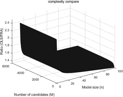89) The ratio of the computational complexity of the fast OLS algorithm in Zhu and Billings (1996) and the computational complexity of the proposed algorithm is illustrated in Figure 3 as a function of the number of candidate terms m and actual model size M. It is graphically shown that the proposed method is computationally more efficient than the fast OLS algorithm in all cases, and the efficiency is much higher as the model size decreases.

Figure 3. The ratio of computational complexities between the fast OLS method and the proposed method.

5. Simulation and analysis

To verify the effectiveness of the proposed method, two simulation examples are used. The first example is a rational model. The second one is the case where the regressors are not all polynomials. For each case, 1000 samples are generated with the same distribution of input and error signals.

The input signals for generating the training and testing samples are independent and uniformly distributed signals with amplitude range $[-1,1]$ and variance of $0.33$ and an independent zero mean Gaussian error with variance $0.01$ is generated as used in Zhu and Billings (1996), S. Chen et al. (1989).

The proposed method is then applied to identify the system defined in Equation (90(90) $\begin{array}{rl}y\left(t\right)& =\frac{a\left(t\right)}{c\left(t\right)}+e\left(t\right)\\ & =\frac{\begin{array}{c}0.25y(t-1)-0.85y(t-2)e(t-2)\\ +u(t-1)u(t-2)\end{array}}{1+0.68y^2(t-1)+y^2(t-2)}+e\left(t\right)\end{array}$(90) ). (90) $\begin{array}{rl}y\left(t\right)& =\frac{a\left(t\right)}{c\left(t\right)}+e\left(t\right)\\ & =\frac{\begin{array}{c}0.25y(t-1)-0.85y(t-2)e(t-2)\\ +u(t-1)u(t-2)\end{array}}{1+0.68y^2(t-1)+y^2(t-2)}+e\left(t\right)\end{array}$(90) The rational fraction system in Equation (90(90) $\begin{array}{rl}y\left(t\right)& =\frac{a\left(t\right)}{c\left(t\right)}+e\left(t\right)\\ & =\frac{\begin{array}{c}0.25y(t-1)-0.85y(t-2)e(t-2)\\ +u(t-1)u(t-2)\end{array}}{1+0.68y^2(t-1)+y^2(t-2)}+e\left(t\right)\end{array}$(90) ) is a typical rational nonlinear autoregressive moving average with eXogenous inputs (NARMAX) model (Waheeb et al., 2019). Models of this kind include past inputs, past outputs and past model errors which are the differences between the estimated values and the true values. Though incorporating the past error signal into the model may lead to a more accurate model, they are often difficult to measure or make the modelling process rather complicated. It should be noted that errors always exist in modelling nonlinear systems (Nelles, 2020). The model error is often decomposed into the bias and the variance. The bias can be decreased to zero by increasing the model nonlinearity, while the variance is significantly influenced by the data size and data quality. Thus the error in Equation (90(90) $\begin{array}{rl}y\left(t\right)& =\frac{a\left(t\right)}{c\left(t\right)}+e\left(t\right)\\ & =\frac{\begin{array}{c}0.25y(t-1)-0.85y(t-2)e(t-2)\\ +u(t-1)u(t-2)\end{array}}{1+0.68y^2(t-1)+y^2(t-2)}+e\left(t\right)\end{array}$(90) ) is often treated as known a priori (Neji & Beji, 2000). In general, the errors are assumed as independent Gaussian random variables with zero mean and a finite variance, and the variance is often given a priori. To this end, in this case study, the variance is set to $0.01$. Accordingly, 27 polynomial terms are generated first based on the principle that the highest order is 2 and the maximal delays of input, error and output signals are 2. According to Equation (7(7) $\mathit{Y}=\mathbf{\Phi }\mathbf{\Theta }+\mathit{c}\odot \mathit{e}=\mathbf{\Phi }\mathbf{\Theta }+\mathbf{\Xi }$(7) ), the candidate terms consist of 54 polynomial regressors.

First, the regularisation parameter is symmetrically adjusted around 0 and a number of trials are tested. Table 1 shows four cases with different values for the regularisation parameter. It is found that $-9$ is the optimal magnitude order for the regularisation parameter in Example 1. Then, the regularisation parameter is fine tuned around the optimal magnitude order, and the final value for the regularisation parameter is chosen to be 1.8276e−9.

Table 1. Different regularisation parameters for Example 1.

Regularisation parameter	$-1e-5$	$-1e-9$	1e−9	1e−5
Selected term	$u(t-1)u(t-2)$	$u(t-1)u(t-2)$	$u(t-1)u(t-2)$	$u(t-1)u(t-2)$
	$y(t-1)$	$y(t-1)$	$y(t-1)$	$y(t-1)$
	$y\left(t\right)\cdot y^2(t-1)$	$y\left(t\right)\cdot y^2(t-2)$	$y\left(t\right)\cdot y^2(t-1)$	$y\left(t\right)\cdot y^2(t-2)$
	$y(t-2)u(t-2)$	$y\left(t\right)\cdot y^2(t-1)$	$y\left(t\right)\cdot y^2(t-2)$	$y\left(t\right)\cdot u^2(t-2)$
	$y(t-2)ϵ(t-2)$	$y(t-2)ϵ(t-2)$	$y\left(t\right)\cdot u^2(t-2)$	$y\left(t\right)\cdot u^2(t-1)$
Estimation parameters	0.9474	0.9977	0.9931	2.4071
	0.2359	0.2471	0.2460	0.4250
	0.6954	0.9722	0.6765	3.4022
	0.0322	0.6772	0.9941	0.0364
	−1.2269	−0.8541	−0.0125	2.6361
MSE of validation	6.5335e–04	9.6952e-05	1.0045e–04	0.0114

Then the rational fraction system in Equation (90(90) $\begin{array}{rl}y\left(t\right)& =\frac{a\left(t\right)}{c\left(t\right)}+e\left(t\right)\\ & =\frac{\begin{array}{c}0.25y(t-1)-0.85y(t-2)e(t-2)\\ +u(t-1)u(t-2)\end{array}}{1+0.68y^2(t-1)+y^2(t-2)}+e\left(t\right)\end{array}$(90) ) is identified by the RFRA algorithm and the fast OLS method in reference Zhu and Billings (1996), respectively. The selected nonlinear terms from the above 54 nonlinear terms and their estimated linear parameters are listed in Table 2. By comparing the parameters obtained by the two algorithms, it is clear that the parameters identified by RFRA algorithm are closer to the actual parameters of the model, and the model obtained is more accurate than that produced by the fast OLS method in reference Zhu and Billings (1996).

Table 2. Comparison of estimation coefficients for Example 1.

Selection order using RFRA	Selected term	True Parameters	Estimated Para-meters using RFRA	Estimated Parameters using OLS
1	$u(t-1)\cdot$	1	0.9977	0.9973
	$u(t-2)$
2	$y(t-1)$	0.25	0.2471	0.269
3	$y\left(t\right)\cdot y^2(t-2)$	1	0.9722	0.963
4	$y\left(t\right)\cdot y^2(t-1)$	0.68	0.6772	0.654
5	$y(t-2)\cdot$	−0.85	−0.8541	−0.613
	$e(t-2)$

Finally, a more general fraction system given in Equation (91(91) $\begin{array}{rl}y\left(t\right)& =\frac{a\left(t\right)}{c\left(t\right)}+e\left(t\right)\\ & =\frac{\begin{array}{c}0.3y(t-1)-0.7y(t-2)\\ +\mathrm{s}\mathrm{i}\mathrm{n}\left(u\right(t-1\left)\right)+u(t-1)\end{array}}{1+\mathrm{e}\mathrm{x}\mathrm{p}(-y^2(t-1\left)\right)+u^2(t-2)}+e\left(t\right)\end{array}$(91) ), which contains both polynomials and other nonlinear terms in the rational function, is used as the second case study. (91) $\begin{array}{rl}y\left(t\right)& =\frac{a\left(t\right)}{c\left(t\right)}+e\left(t\right)\\ & =\frac{\begin{array}{c}0.3y(t-1)-0.7y(t-2)\\ +\mathrm{s}\mathrm{i}\mathrm{n}\left(u\right(t-1\left)\right)+u(t-1)\end{array}}{1+\mathrm{e}\mathrm{x}\mathrm{p}(-y^2(t-1\left)\right)+u^2(t-2)}+e\left(t\right)\end{array}$(91) Similarly, nonlinear candidate items are generated. Considering the small number of samples which is only 1000, different basis functions are used as the numerator and denominator candidate terms, leading to the generation of 52 candidate terms.

It is shown that the bias becomes greater in the positive direction in Example 1, hence, similarly the regularisation parameter is fine tuned along the negative values for Example 2. Following the same procedure in example 1, the regularisation parameter is firstly coarsely adjusted and Table 3 shows some cases with different values for the regularisation parameter. After numerous trials, it is evident again that $-9$ is the optimum magnitude order for the regularisation parameter. Then, the regularisation parameter is further fine tuned. It is noted that the magnitude order of the MSE validation errors in all the two examples could achieve to $-4$ even without fine-tuning. The nonlinear regressors are selected and the coefficients are estimated which are shown in Table 4. It is again evident that the fraction system can be well identified using the proposed method.

Table 3. Different regularisation parameters for Example 2.

Regularisation parameter	$-1e-9$	$-1e-6$	0	1e−14
Selected term	$u(t-1)$	$u(t-1)$	$u(t-1)$	$u(t-1)$
	$y(t-2)$	$y(t-2)$	$y(t-2)$	$y(t-2)$
	$y(t-1)$	$y(t-1)$	$y(t-1)$	$y(t-1)$
	$\mathrm{s}\mathrm{i}\mathrm{n}\left(u\right(t-1\left)\right)$	$\mathrm{s}\mathrm{i}\mathrm{n}\left(u\right(t-1\left)\right)$	$\mathrm{s}\mathrm{i}\mathrm{n}\left(u\right(t-1\left)\right)$	$\mathrm{s}\mathrm{i}\mathrm{n}\left(u\right(t-1\left)\right)$
	$y\left(t\right)\cdot u^2(t-2)$	$y\left(t\right)\cdot u^2(t-2)$	$y\left(t\right)\cdot u^2(i-2)$	$y\left(t\right)\cdot u^2(t-2)$
	$y\left(t\right)\cdot$	$y\left(t\right)\cdot y(t-2)\cdot$	$y\left(t\right)\cdot \mathrm{e}\mathrm{x}\mathrm{p}(-u(t-1)\cdot$	$y\left(t\right)\cdot \mathrm{e}\mathrm{x}\mathrm{p}(-u(t-1)\cdot$
	$\mathrm{e}\mathrm{x}\mathrm{p}(-y(t-1{)}^2)$	$u(t-2))$	$u(t-2))$	$u(t-2))$
Estimation Parameters	0.9359	0.5795	1.5871	1.5871
	−0.6642	−0.3586	−0.5697	−0.5697
	0.2825	0.1573	0.243	0.243
	0.9068	0.1828	0.7952	0.7952
	0.8935	−0.0553	0.7864	0.7863
	0.9597	0.4437	−0.2129	−0.2129
MSE of Validation	1.0693e–04	0.0016	1.3552e–04	1.3552e–04

Table 4. Structure selection and parameters estimation for Example 2.

Selection order	Selected term	True parameters	Estimated parameters
1	$u(t-1)$	1	0.9611
2	$y(t-2)$	−0.7	−0.6728
3	$y(t-1)$	0.3	0.2871
4	$u^2(t-2)$	1	0.9299
5	$\mathrm{e}\mathrm{x}\mathrm{p}(-y^2(t-1\left)\right)$	1	0.9210
6	$\mathrm{s}\mathrm{i}\mathrm{n}\left(u\right(t-1\left)\right)$	1	0.9618

6. Conclusion

This paper has proposed a novel fast method to identify the fraction models where the model structure and the coefficients are simultaneously estimated. The identification of the fraction system is first transformed to an equivalent quadratic optimisation problem by adding a regularisation term which is formulated as the inner product of the denominator terms. To solve the quadratic optimisation problem, a regularised fast recursive algorithm is developed. The proposed method is further validated by two simulation examples to confirm its efficacy. The method can be further applied to build the output layer of the traditional neural networks or the full connected layer of the deep neural networks which can reduce the size of the neural networks. However, a potential limitation of the proposed method is the computational effort to fine tune the regularisation parameter though we have shown that it value has to be negative and can not exceed ${\mathit{Y}}^{\mathrm{T}}\mathit{Y}$. It will inevitably cost more computations to optimise the regularisation parameter if the system is too complex. Fast optimisation of the penalty parameter will be a future research topic.

Disclosure statement

No potential conflict of interest was reported by the author(s).

Data availability statement

The authors confirm that the data supporting the findings of this study are available within the article.

Additional information

Funding

This work is supported by Key Project of Science and Technology Commission of Shanghai Municipality [No. 19500712300], 111 Project [No. D18003].

Notes on contributors

Li Zhang

Li Zhang received the B.Sc. and M.Sc. degrees from Anhui University of Technology, Anhui, China, in 2009 and 2013, respectively. She is currently pursuing the Ph.D. degree in control theory and control engineering at Shanghai University. Between 2018 and 2019, she was a visiting Ph.D. student with the University of Leeds, U.K. Her current research interests include nonlinear system modeling and identification, machine learning algorithm and power system.

Kang Li

Kang Li (M'05-SM'11) received the B.Sc. degree in Industrial Automation from Xiangtan University, Hunan, China, in 1989, the M.Sc. degree in Control Theory and Applications from Harbin Institute of Technology, Harbin, China, in 1992, and the Ph.D. degree in Control Theory and Applications from Shanghai Jiaotong University, Shanghai, China, in 1995. He also received D.Sc. degree in system identification from Queen's University Belfast, UK, in 2015. Between 1995 and 2002, he worked at Shanghai Jiaotong University, Delft University of Technology and Queen's University Belfast as a research fellow. Between 2002 and 2018, he was a Lecturer (2002), a Senior Lecturer (2007), a Reader (2009) and a Chair Professor (2011) with the School of Electronics, Electrical Engineering and Computer Science, Queen's University Belfast, Belfast, U.K. He currently holds the Chair of Smart Energy Systems at the University of Leeds, UK. His research interests cover nonlinear system modelling, identification, and control, and machine learning, with substantial applications to energy and power systems, smart grid, electric vehicles, railway systems, and energy management in energy intensive manufacturing processes. He has authored/co-authored over 200 journal publications and edited/co-edited 19 conference proceedings.

Dr Li chaired the IEEE UKRI Control and Communication Ireland chapter, and was the Secretary of the IEEE UK & Ireland Section.

Dajun Du

Dajun Du received the B.Sc. degree in electrical technology, and M.Sc. degrees in control theory and control engineering all from the Zhengzhou University, China in 2002 and 2005, respectively, and his Ph. D. degree in control theory and control engineering from Shanghai University in 2010. From September 2008 to September 2009, he was a visiting PhD student at Queen's University Belfast, UK. From April 2011 to August 2012, he was a Research Fellow at Queen's University Belfast, UK. He is currently a professor in Shanghai University. His main research interests include system modelling and identification and networked control systems.

Yihuan Li

Yihuan Li received the B.Sc. and M.Sc. degrees from North China Electric Power University, Beijing, China, in 2014 and 2017, respectively, and the PhD degree from University of Leeds in 2021. She is currently a lecture in North China Electric Power University. Her main research interests include system identification and state estimation, and the application of machine learning techniques in the field of battery management.

Minrui Fei

Minrui Fei received his B.S. and M.S. degrees in Industrial Automation from the Shanghai University of Technology in 1984 and 1992, respectively, and his PhD degree in Control Theory and Control Engineering from Shanghai University in 1997. Since 1998, he has been a full professor at Shanghai University. He is Chairman of Embedded Instrument and System Sub-society, and Standing Director of China Instrument & Control Society; Chairman of Life System Modeling and Simulation Sub-society, Vice-chairman of Intelligent Control and Intelligent Management Sub-society, and Director of Chinese Artificial Intelligence Association. His research interests are in the areas of networked control systems, intelligent control, complex system modeling, hybrid network systems, and field control systems.

Appendices

Appendix 1.

Simplifying the regularized cost function

According to the principles of matrix manipulation, the cost function is simplified in Equation (A1(A1) $\begin{array}{rl}\mathit{J}& ={\mathit{Y}}^{\mathrm{T}}\mathit{Y}-{\mathbf{\Theta }}^{\mathrm{T}}{\mathbf{\Phi }}^{\mathrm{T}}\mathit{Y}-{\mathit{Y}}^{\mathrm{T}}\mathbf{\Phi }\mathbf{\Theta }+{\mathbf{\Theta }}^{\mathrm{T}}{\mathbf{\Phi }}^{\mathrm{T}}\mathbf{\Phi }\mathbf{\Theta }\\ & +\lambda {\mathbf{\Theta }}^{\mathrm{T}}{\mathbf{\Psi }}^{\mathrm{T}}\mathbf{\Psi }\mathbf{\Theta }+\lambda {\mathbf{\Theta }}^{\mathrm{T}}{\mathbf{\Psi }}^{\mathrm{T}}\mathit{E}+\lambda {\mathit{E}}^{\mathrm{T}}\mathbf{\Psi }\mathbf{\Theta }\\ & ={\mathit{Y}}^{\mathrm{T}}\mathit{Y}-({\mathit{Y}}^{\mathrm{T}}\mathbf{\Phi }-\lambda {\mathit{E}}^{\mathrm{T}}\mathbf{\Psi })({\mathbf{\Phi }}^{\mathrm{T}}\mathbf{\Phi }+\lambda {\mathbf{\Psi }}^{\mathrm{T}}\mathbf{\Psi }{)}^{-1}{\mathbf{\Phi }}^{\mathrm{T}}\mathit{Y}\\ & +\lambda {\mathit{E}}^{\mathrm{T}}\mathit{E}-{\mathit{Y}}^{\mathrm{T}}\mathbf{\Phi }({\mathbf{\Phi }}^{\mathrm{T}}\mathbf{\Phi }+\lambda {\mathbf{\Psi }}^{\mathrm{T}}\mathbf{\Psi }{)}^{-1}({\mathbf{\Phi }}^{\mathrm{T}}\mathit{Y}-\lambda {\mathbf{\Psi }}^{\mathrm{T}}\mathit{E})\\ & +({\mathit{Y}}^{\mathrm{T}}\mathbf{\Phi }-\lambda {\mathit{E}}^{\mathrm{T}}\mathbf{\Psi })({\mathbf{\Phi }}^{\mathrm{T}}\mathbf{\Phi }+\lambda {\mathbf{\Psi }}^{\mathrm{T}}\mathbf{\Psi }{)}^{-1}\\ & \times {\mathbf{\Phi }}^{\mathrm{T}}\mathbf{\Phi }({\mathbf{\Phi }}^{\mathrm{T}}\mathbf{\Phi }+\lambda {\mathbf{\Psi }}^{\mathrm{T}}\mathbf{\Psi }{)}^{-1}({\mathbf{\Phi }}^{\mathrm{T}}\mathit{Y}-\lambda {\mathbf{\Psi }}^{\mathrm{T}}\mathit{E})\\ & +\lambda ({\mathit{Y}}^{\mathrm{T}}\mathbf{\Phi }-\lambda {\mathit{E}}^{\mathrm{T}}\mathbf{\Psi })({\mathbf{\Phi }}^{\mathrm{T}}\mathbf{\Phi }+\lambda {\mathbf{\Psi }}^{\mathrm{T}}\mathbf{\Psi }{)}^{-1}\\ & \times {\mathbf{\Psi }}^{\mathrm{T}}\mathbf{\Psi }({\mathbf{\Phi }}^{\mathrm{T}}\mathbf{\Phi }+\lambda {\mathbf{\Psi }}^{\mathrm{T}}\mathbf{\Psi }{)}^{-1}({\mathbf{\Phi }}^{\mathrm{T}}\mathit{Y}-\lambda {\mathbf{\Psi }}^{\mathrm{T}}\mathit{E})\\ & +\lambda ({\mathit{Y}}^{\mathrm{T}}\mathbf{\Phi }-\lambda {\mathit{E}}^{\mathrm{T}}\mathbf{\Psi })({\mathbf{\Phi }}^{\mathrm{T}}\mathbf{\Phi }+\lambda {\mathbf{\Psi }}^{\mathrm{T}}\mathbf{\Psi }{)}^{-1}{\mathbf{\Psi }}^{\mathrm{T}}\mathit{E}\\ & +\lambda {\mathit{E}}^{\mathrm{T}}\mathbf{\Psi }({\mathbf{\Phi }}^{\mathrm{T}}\mathbf{\Phi }+\lambda {\mathbf{\Psi }}^{\mathrm{T}}\mathbf{\Psi }{)}^{-1}({\mathbf{\Phi }}^{\mathrm{T}}\mathit{Y}+\lambda {\mathbf{\Psi }}^{\mathrm{T}}\mathit{E})-\lambda {\mathit{E}}^{\mathrm{T}}\mathit{E}\end{array}$(A1) ). (A1) $\begin{array}{rl}\mathit{J}& ={\mathit{Y}}^{\mathrm{T}}\mathit{Y}-{\mathbf{\Theta }}^{\mathrm{T}}{\mathbf{\Phi }}^{\mathrm{T}}\mathit{Y}-{\mathit{Y}}^{\mathrm{T}}\mathbf{\Phi }\mathbf{\Theta }+{\mathbf{\Theta }}^{\mathrm{T}}{\mathbf{\Phi }}^{\mathrm{T}}\mathbf{\Phi }\mathbf{\Theta }\\ & +\lambda {\mathbf{\Theta }}^{\mathrm{T}}{\mathbf{\Psi }}^{\mathrm{T}}\mathbf{\Psi }\mathbf{\Theta }+\lambda {\mathbf{\Theta }}^{\mathrm{T}}{\mathbf{\Psi }}^{\mathrm{T}}\mathit{E}+\lambda {\mathit{E}}^{\mathrm{T}}\mathbf{\Psi }\mathbf{\Theta }\\ & ={\mathit{Y}}^{\mathrm{T}}\mathit{Y}-({\mathit{Y}}^{\mathrm{T}}\mathbf{\Phi }-\lambda {\mathit{E}}^{\mathrm{T}}\mathbf{\Psi })({\mathbf{\Phi }}^{\mathrm{T}}\mathbf{\Phi }+\lambda {\mathbf{\Psi }}^{\mathrm{T}}\mathbf{\Psi }{)}^{-1}{\mathbf{\Phi }}^{\mathrm{T}}\mathit{Y}\\ & +\lambda {\mathit{E}}^{\mathrm{T}}\mathit{E}-{\mathit{Y}}^{\mathrm{T}}\mathbf{\Phi }({\mathbf{\Phi }}^{\mathrm{T}}\mathbf{\Phi }+\lambda {\mathbf{\Psi }}^{\mathrm{T}}\mathbf{\Psi }{)}^{-1}({\mathbf{\Phi }}^{\mathrm{T}}\mathit{Y}-\lambda {\mathbf{\Psi }}^{\mathrm{T}}\mathit{E})\\ & +({\mathit{Y}}^{\mathrm{T}}\mathbf{\Phi }-\lambda {\mathit{E}}^{\mathrm{T}}\mathbf{\Psi })({\mathbf{\Phi }}^{\mathrm{T}}\mathbf{\Phi }+\lambda {\mathbf{\Psi }}^{\mathrm{T}}\mathbf{\Psi }{)}^{-1}\\ & \times {\mathbf{\Phi }}^{\mathrm{T}}\mathbf{\Phi }({\mathbf{\Phi }}^{\mathrm{T}}\mathbf{\Phi }+\lambda {\mathbf{\Psi }}^{\mathrm{T}}\mathbf{\Psi }{)}^{-1}({\mathbf{\Phi }}^{\mathrm{T}}\mathit{Y}-\lambda {\mathbf{\Psi }}^{\mathrm{T}}\mathit{E})\\ & +\lambda ({\mathit{Y}}^{\mathrm{T}}\mathbf{\Phi }-\lambda {\mathit{E}}^{\mathrm{T}}\mathbf{\Psi })({\mathbf{\Phi }}^{\mathrm{T}}\mathbf{\Phi }+\lambda {\mathbf{\Psi }}^{\mathrm{T}}\mathbf{\Psi }{)}^{-1}\\ & \times {\mathbf{\Psi }}^{\mathrm{T}}\mathbf{\Psi }({\mathbf{\Phi }}^{\mathrm{T}}\mathbf{\Phi }+\lambda {\mathbf{\Psi }}^{\mathrm{T}}\mathbf{\Psi }{)}^{-1}({\mathbf{\Phi }}^{\mathrm{T}}\mathit{Y}-\lambda {\mathbf{\Psi }}^{\mathrm{T}}\mathit{E})\\ & +\lambda ({\mathit{Y}}^{\mathrm{T}}\mathbf{\Phi }-\lambda {\mathit{E}}^{\mathrm{T}}\mathbf{\Psi })({\mathbf{\Phi }}^{\mathrm{T}}\mathbf{\Phi }+\lambda {\mathbf{\Psi }}^{\mathrm{T}}\mathbf{\Psi }{)}^{-1}{\mathbf{\Psi }}^{\mathrm{T}}\mathit{E}\\ & +\lambda {\mathit{E}}^{\mathrm{T}}\mathbf{\Psi }({\mathbf{\Phi }}^{\mathrm{T}}\mathbf{\Phi }+\lambda {\mathbf{\Psi }}^{\mathrm{T}}\mathbf{\Psi }{)}^{-1}({\mathbf{\Phi }}^{\mathrm{T}}\mathit{Y}+\lambda {\mathbf{\Psi }}^{\mathrm{T}}\mathit{E})-\lambda {\mathit{E}}^{\mathrm{T}}\mathit{E}\end{array}$(A1) $\begin{array}{rl}& ={\mathit{Y}}^{\mathrm{T}}\mathit{Y}-{\mathit{Y}}^{\mathrm{T}}\mathbf{\Phi }({\mathbf{\Phi }}^{\mathrm{T}}\mathbf{\Phi }+\lambda {\mathbf{\Psi }}^{\mathrm{T}}\mathbf{\Psi }{)}^{-1}{\mathbf{\Phi }}^{\mathrm{T}}\mathit{Y}\\ & +\lambda {\mathit{E}}^{\mathrm{T}}\mathbf{\Psi }({\mathbf{\Phi }}^{\mathrm{T}}\mathbf{\Phi }+\lambda {\mathbf{\Psi }}^{\mathrm{T}}\mathbf{\Psi }{)}^{-1}{\mathbf{\Phi }}^{\mathrm{T}}\mathit{Y}\\ & +\lambda {\mathit{E}}^{\mathrm{T}}\mathit{E}-{\mathit{Y}}^{\mathrm{T}}\mathbf{\Phi }({\mathbf{\Phi }}^{\mathrm{T}}\mathbf{\Phi }+\lambda {\mathbf{\Psi }}^{\mathrm{T}}\mathbf{\Psi }{)}^{-1}{\mathbf{\Phi }}^{\mathrm{T}}\mathit{Y}\\ & +\lambda {\mathit{Y}}^{\mathrm{T}}\mathbf{\Phi }({\mathbf{\Phi }}^{\mathrm{T}}\mathbf{\Phi }+\lambda {\mathbf{\Psi }}^{\mathrm{T}}\mathbf{\Psi }{)}^{-1}{\mathbf{\Psi }}^{\mathrm{T}}\mathit{E}\\ & +({\mathit{Y}}^{\mathrm{T}}\mathbf{\Phi }-\lambda {\mathit{E}}^{\mathrm{T}}\mathbf{\Psi })({\mathbf{\Phi }}^{\mathrm{T}}\mathbf{\Phi }+\lambda {\mathbf{\Psi }}^{\mathrm{T}}\mathbf{\Psi }{)}^{-1}({\mathbf{\Phi }}^{\mathrm{T}}\mathbf{\Phi }+\lambda {\mathbf{\Psi }}^{\mathrm{T}}\mathbf{\Psi })\\ & \times ({\mathbf{\Phi }}^{\mathrm{T}}\mathbf{\Phi }+\lambda {\mathbf{\Psi }}^{\mathrm{T}}\mathbf{\Psi }{)}^{-1}({\mathbf{\Phi }}^{\mathrm{T}}\mathit{Y}-\lambda {\mathbf{\Psi }}^{\mathrm{T}}\mathit{E})\\ & +\lambda {\mathit{Y}}^{\mathrm{T}}\mathbf{\Phi }({\mathbf{\Phi }}^{\mathrm{T}}\mathbf{\Phi }+\lambda {\mathbf{\Psi }}^{\mathrm{T}}\mathbf{\Psi }{)}^{-1}{\mathbf{\Psi }}^{\mathrm{T}}\mathit{E}\\ & -\lambda {\mathit{E}}^{\mathrm{T}}\mathbf{\Psi }({\mathbf{\Phi }}^{\mathrm{T}}\mathbf{\Phi }+\lambda {\mathbf{\Psi }}^{\mathrm{T}}\mathbf{\Psi }{)}^{-1}\lambda {\mathbf{\Psi }}^{\mathrm{T}}\mathit{E}\\ & +\lambda {\mathit{E}}^{\mathrm{T}}\mathbf{\Psi }({\mathbf{\Phi }}^{\mathrm{T}}\mathbf{\Phi }+\lambda {\mathbf{\Psi }}^{\mathrm{T}}\mathbf{\Psi }{)}^{-1}{\mathbf{\Phi }}^{\mathrm{T}}\mathit{Y}\\ & -\lambda {\mathit{E}}^{\mathrm{T}}\mathbf{\Psi }({\mathbf{\Phi }}^{\mathrm{T}}\mathbf{\Phi }+\lambda {\mathbf{\Psi }}^{\mathrm{T}}\mathbf{\Psi }{)}^{-1}\lambda {\mathbf{\Psi }}^{\mathrm{T}}\mathit{E}\\ & ={\mathit{Y}}^{\mathrm{T}}\mathit{Y}+\lambda {\mathit{E}}^{\mathrm{T}}\mathit{E}-2{\mathit{Y}}^{\mathrm{T}}\mathbf{\Phi }({\mathbf{\Phi }}^{\mathrm{T}}\mathbf{\Phi }+\lambda {\mathbf{\Psi }}^{\mathrm{T}}\mathbf{\Psi }{)}^{-1}{\mathbf{\Phi }}^{\mathrm{T}}\mathit{Y}\\ & +4\lambda {\mathit{E}}^{\mathrm{T}}\mathbf{\Psi }({\mathbf{\Phi }}^{\mathrm{T}}\mathbf{\Phi }+\lambda {\mathbf{\Psi }}^{\mathrm{T}}\mathbf{\Psi }{)}^{-1}{\mathbf{\Phi }}^{\mathrm{T}}\mathit{Y}\\ & +({\mathit{Y}}^{\mathrm{T}}\mathbf{\Phi }-\lambda {\mathit{E}}^{\mathrm{T}}\mathbf{\Psi })({\mathbf{\Phi }}^{\mathrm{T}}\mathbf{\Phi }+\lambda {\mathbf{\Psi }}^{\mathrm{T}}\mathbf{\Psi }{)}^{-1}({\mathbf{\Phi }}^{\mathrm{T}}\mathit{Y}-\lambda {\mathbf{\Psi }}^{\mathrm{T}}\mathit{E})\\ & -2\lambda {\mathit{E}}^{\mathrm{T}}\mathbf{\Psi }({\mathbf{\Phi }}^{\mathrm{T}}\mathbf{\Phi }+\lambda {\mathbf{\Psi }}^{\mathrm{T}}\mathbf{\Psi }{)}^{-1}\lambda {\mathbf{\Psi }}^{\mathrm{T}}\mathit{E}\\ & ={\mathit{Y}}^{\mathrm{T}}\mathit{Y}+\lambda {\mathit{E}}^{\mathrm{T}}\mathit{E}-2{\mathit{Y}}^{\mathrm{T}}\mathbf{\Phi }({\mathbf{\Phi }}^{\mathrm{T}}\mathbf{\Phi }+\lambda {\mathbf{\Psi }}^{\mathrm{T}}\mathbf{\Psi }{)}^{-1}{\mathbf{\Phi }}^{\mathrm{T}}\mathit{Y}\\ & +4\lambda {\mathit{E}}^{\mathrm{T}}\mathbf{\Psi }({\mathbf{\Phi }}^{\mathrm{T}}\mathbf{\Phi }+\lambda {\mathbf{\Psi }}^{\mathrm{T}}\mathbf{\Psi }{)}^{-1}{\mathbf{\Phi }}^{\mathrm{T}}\mathit{Y}\\ & +{\mathit{Y}}^{\mathrm{T}}\mathbf{\Phi }({\mathbf{\Phi }}^{\mathrm{T}}\mathbf{\Phi }+\lambda {\mathbf{\Psi }}^{\mathrm{T}}\mathbf{\Psi }{)}^{-1}{\mathbf{\Phi }}^{\mathrm{T}}\mathit{Y}\\ & -{\mathit{Y}}^{\mathrm{T}}\mathbf{\Phi }({\mathbf{\Phi }}^{\mathrm{T}}\mathbf{\Phi }+\lambda {\mathbf{\Psi }}^{\mathrm{T}}\mathbf{\Psi }{)}^{-1}\lambda {\mathbf{\Psi }}^{\mathrm{T}}\mathit{E}\\ & -\lambda {\mathit{E}}^{\mathrm{T}}\mathbf{\Psi }({\mathbf{\Phi }}^{\mathrm{T}}\mathbf{\Phi }+\lambda {\mathbf{\Psi }}^{\mathrm{T}}\mathbf{\Psi }{)}^{-1}{\mathbf{\Phi }}^{\mathrm{T}}\mathit{Y}\\ & +\lambda {\mathit{E}}^{\mathrm{T}}\mathbf{\Psi }({\mathbf{\Phi }}^{\mathrm{T}}\mathbf{\Phi }+\lambda {\mathbf{\Psi }}^{\mathrm{T}}\mathbf{\Psi }{)}^{-1}\lambda {\mathbf{\Psi }}^{\mathrm{T}}\mathit{E}\\ & -2\lambda {\mathit{E}}^{\mathrm{T}}\mathbf{\Psi }({\mathbf{\Phi }}^{\mathrm{T}}\mathbf{\Phi }+\lambda {\mathbf{\Psi }}^{\mathrm{T}}\mathbf{\Psi }{)}^{-1}\lambda {\mathbf{\Psi }}^{\mathrm{T}}\mathit{E}\end{array}$ $\begin{array}{rl}& ={\mathit{Y}}^{\mathrm{T}}\mathit{Y}+\lambda {\mathit{E}}^{\mathrm{T}}\mathit{E}-{\mathit{Y}}^{\mathrm{T}}\mathbf{\Phi }({\mathbf{\Phi }}^{\mathrm{T}}\mathbf{\Phi }+\lambda {\mathbf{\Psi }}^{\mathrm{T}}\mathbf{\Psi }{)}^{-1}{\mathbf{\Phi }}^{\mathrm{T}}\mathit{Y}\\ & +2\lambda {\mathit{E}}^{\mathrm{T}}\mathbf{\Psi }({\mathbf{\Phi }}^{\mathrm{T}}\mathbf{\Phi }+\lambda {\mathbf{\Psi }}^{\mathrm{T}}\mathbf{\Psi }{)}^{-1}{\mathbf{\Phi }}^{\mathrm{T}}\mathit{Y}\\ & -\lambda {\mathit{E}}^{\mathrm{T}}\mathbf{\Psi }({\mathbf{\Phi }}^{\mathrm{T}}\mathbf{\Phi }+\lambda {\mathbf{\Psi }}^{\mathrm{T}}\mathbf{\Psi }{)}^{-1}\lambda {\mathbf{\Psi }}^{\mathrm{T}}\mathit{E}\\ & ={\mathit{Y}}^{\mathrm{T}}(\mathit{I}-\mathbf{\Phi }({\mathbf{\Phi }}^{\mathrm{T}}\mathbf{\Phi }+\lambda {\mathbf{\Psi }}^{\mathrm{T}}\mathbf{\Psi }{)}^{-1}{\mathbf{\Phi }}^{\mathrm{T}})\mathit{Y}\\ & +2\lambda {\mathit{Y}}^{\mathrm{T}}\mathbf{\Psi }({\mathbf{\Phi }}^{\mathrm{T}}\mathbf{\Phi }+\lambda {\mathbf{\Psi }}^{\mathrm{T}}\mathbf{\Psi }{)}^{-1}{\mathbf{\Phi }}^{\mathrm{T}}\mathit{E}\\ & +\lambda {\mathit{E}}^{\mathrm{T}}(\mathit{I}-\lambda \mathbf{\Psi }({\mathbf{\Phi }}^{\mathrm{T}}\mathbf{\Phi }+\lambda {\mathbf{\Psi }}^{\mathrm{T}}\mathbf{\Psi }{)}^{-1}{\mathbf{\Psi }}^{\mathrm{T}})\mathit{E}\end{array}$

Appendix 2.

Proof of Properties of the recursive matrices

From the definition of $M_k^{-1}$ in Equation (29(29) $\begin{array}{rl}{\mathit{M}}_k^{-1}& ={\left[\begin{array}{cc}{\mathit{M}}_{k-1}& \begin{array}{c}{\mathbf{\Phi }}_{k-1}^{\mathrm{T}}{\mathit{\varphi }}_k\\ +\lambda {\mathbf{\Psi }}_{k-1}^{\mathrm{T}}{\mathit{\psi }}_k\end{array}\\ {\mathit{\varphi }}_k^{\mathrm{T}}{\mathbf{\Phi }}_{k-1}+\lambda {\mathit{\psi }}_k^{\mathrm{T}}{\mathbf{\Psi }}_{k-1}& {\mathit{\varphi }}_k^{\mathrm{T}}{\mathit{\varphi }}_k+\lambda {\mathit{\psi }}_k^{\mathrm{T}}{\mathit{\psi }}_k\end{array}\right]}^{-1}\\ & =\left[\begin{array}{cc}{\mathit{F}}_{k-1}& {\mathit{g}}_{k-1}\\ {\mathit{g}}_{k-1}^{\mathrm{T}}& {\mathit{f}}_{k-1}\end{array}\right]\end{array}$(29) ), substituting Equations (30(30) $\{\begin{array}{l}{\displaystyle {\mathit{F}}_{k-1}=[{\mathit{M}}_{k-1}-({\mathbf{\Phi }}_{k-1}^{\mathrm{T}}{\mathit{\varphi }}_k+\lambda {\mathbf{\Psi }}_{k-1}^{\mathrm{T}}{\mathit{\psi }}_k)}\\ ({\mathit{\varphi }}_k^{\mathrm{T}}{\mathbf{\Phi }}_{k-1}+\lambda {\mathit{\psi }}_k^{\mathrm{T}}{\mathbf{\Psi }}_{k-1})/({\mathit{\varphi }}_k^{\mathrm{T}}{\mathit{\varphi }}_k+\lambda {\mathit{\psi }}_k^{\mathrm{T}}{\mathit{\psi }}_k){]}^{-1}\\ {\displaystyle {\mathit{g}}_{k-1}=-{\mathit{F}}_{k-1}({\mathbf{\Phi }}_{k-1}^{\mathrm{T}}{\mathit{\varphi }}_k+\lambda {\mathbf{\Psi }}_{k-1}^{\mathrm{T}}{\mathit{\psi }}_k)}\\ /({\mathit{\varphi }}_k^{\mathrm{T}}{\mathit{\varphi }}_k+\lambda {\mathit{\psi }}_k^{\mathrm{T}}{\mathit{\psi }}_k)\\ {\displaystyle {\mathit{f}}_{k-1}=\frac{\begin{array}{c}({\mathit{\varphi }}_k^{\mathrm{T}}{\mathit{\varphi }}_k+\lambda {\mathit{\psi }}_k^{\mathrm{T}}{\mathit{\psi }}_k)\\ +({\mathit{\varphi }}_k^{\mathrm{T}}{\mathbf{\Phi }}_{k-1}+\lambda {\mathit{\psi }}_k^{\mathrm{T}}{\mathbf{\Psi }}_{k-1}){\mathit{F}}_{k-1}\\ ({\mathbf{\Phi }}_{k-1}^{\mathrm{T}}{\mathit{\varphi }}_k+\lambda {\mathbf{\Psi }}_{k-1}^{\mathrm{T}}{\mathit{\psi }}_k)\end{array}}{({\mathit{\varphi }}_k^{\mathrm{T}}{\mathit{\varphi }}_k+\lambda {\mathit{\psi }}_k^{\mathrm{T}}{\mathit{\psi }}_k{)}^2}}\end{array}$(30) ) and (31(31) ${\mathit{F}}_{k-1}={\mathit{M}}_{k-1}^{-1}+\frac{\begin{array}{c}{\mathit{M}}_{k-1}^{-1}({\mathbf{\Phi }}_{k-1}^{\mathrm{T}}{\mathit{\varphi }}_k+\lambda {\mathbf{\Psi }}_{k-1}^{\mathrm{T}}{\mathit{\psi }}_k)\\ ({\mathit{\varphi }}_k^{\mathrm{T}}{\mathbf{\Phi }}_{k-1}+\lambda {\mathit{\psi }}_k^{\mathrm{T}}{\mathbf{\Psi }}_{k-1}){\mathit{M}}_{k-1}^{-1}\end{array}}{\begin{array}{c}{\mathit{\varphi }}_k^{\mathrm{T}}{\mathit{\varphi }}_k+\lambda {\mathit{\psi }}_k^{\mathrm{T}}{\mathit{\psi }}_k\\ -({\mathit{\varphi }}_k^{\mathrm{T}}{\mathbf{\Phi }}_{k-1}+\lambda {\mathit{\psi }}_k^{\mathrm{T}}{\mathbf{\Psi }}_{k-1}){\mathit{M}}_{k-1}^{-1}\\ ({\mathbf{\Phi }}_{k-1}^{\mathrm{T}}{\mathit{\varphi }}_k+\lambda {\mathbf{\Psi }}_{k-1}^{\mathrm{T}}{\mathit{\psi }}_k)\end{array}}$(31) ) to the definition of $R_{k+1}^{\left(1\right)}$ in Equation (35(35) $\begin{array}{rl}{\mathit{R}}_{k+1}^{\left(1\right)}& \triangleq \mathit{I}-{\mathbf{\Phi }}_{k+1}{\mathit{M}}_{k+1}^{-1}{\mathbf{\Phi }}_{k+1}^{\mathrm{T}}\end{array}$(35) ), the recursive formulation of $R_{k+1}^{\left(1\right)}$ is given in Equation (A2(A2) $\begin{array}{rl}& -\frac{\begin{array}{c}{\mathit{\varphi }}_{k+1}({\mathit{\varphi }}_{k+1}^{\mathrm{T}}{\mathbf{\Phi }}_k+\lambda {\mathit{\psi }}_{k+1}^{\mathrm{T}}{\mathbf{\Psi }}_k){\mathit{M}}_k^{-1}{\mathbf{\Phi }}_k^{\mathrm{T}}\\ -{\mathbf{\Phi }}_k{\mathit{M}}_k^{-1}({\mathbf{\Phi }}_k^{\mathrm{T}}{\mathit{\varphi }}_{k+1}+\lambda {\mathbf{\Psi }}_k^{\mathrm{T}}{\mathit{\psi }}_{k+1})\\ {\mathit{\varphi }}_{k+1}^{\mathrm{T}}+{\mathit{\varphi }}_{k+1}{\mathit{\varphi }}_{k+1}^{\mathrm{T}}\end{array}}{\begin{array}{c}({\mathit{\varphi }}_{k+1}^{\mathrm{T}}{\mathit{\varphi }}_{k+1}+\lambda {\mathit{\psi }}_{k+1}^{\mathrm{T}}{\mathit{\psi }}_{k+1}\\ -({\mathit{\varphi }}_{k+1}^{\mathrm{T}}{\mathbf{\Phi }}_k+\lambda {\mathit{\psi }}_{k+1}^{\mathrm{T}}{\mathbf{\Psi }}_k){\mathit{M}}_k^{-1}\\ ({\mathbf{\Phi }}_k^{\mathrm{T}}{\mathit{\varphi }}_{k+1}+\lambda {\mathbf{\Psi }}_k^{\mathrm{T}}{\mathit{\psi }}_{k+1}))\end{array}}\\ & =\frac{\begin{array}{c}\left({\mathbf{\Phi }}_k{\mathit{M}}_k^{-1}\right({\mathbf{\Phi }}_k^{\mathrm{T}}{\mathit{\varphi }}_{k+1}+\lambda {\mathbf{\Psi }}_k^{\mathrm{T}}{\mathit{\psi }}_{k+1})\\ -{\mathit{\varphi }}_{k+1}\left)\right(({\mathit{\varphi }}_{k+1}^{\mathrm{T}}{\mathbf{\Phi }}_k+\lambda {\mathit{\psi }}_{k+1}^{\mathrm{T}}{\mathbf{\Psi }}_k)\\ {\mathit{M}}_k^{-1}{\mathbf{\Phi }}_k^{\mathrm{T}}-{\mathit{\varphi }}_{k+1}^{\mathrm{T}})\end{array}}{\begin{array}{c}({\mathit{\varphi }}_{k+1}^{\mathrm{T}}{\mathit{\varphi }}_{k+1}+\lambda {\mathit{\psi }}_{k+1}^{\mathrm{T}}{\mathit{\psi }}_{k+1}\\ -({\mathit{\varphi }}_{k+1}^{\mathrm{T}}{\mathbf{\Phi }}_k+\lambda {\mathit{\psi }}_{k+1}^{\mathrm{T}}{\mathbf{\Psi }}_k){\mathit{M}}_k^{-1}\\ ({\mathbf{\Phi }}_k^{\mathrm{T}}{\mathit{\varphi }}_{k+1}+\lambda {\mathbf{\Psi }}_k^{\mathrm{T}}{\mathit{\psi }}_{k+1}))\end{array}}\\ & =\frac{\begin{array}{c}({\mathit{R}}_k^{\left(1\right)}{\mathit{\varphi }}_{k+1}+\lambda {\mathit{R}}_k^{\left(3\right)}{\mathit{\psi }}_{k+1})\\ \left({\mathit{\varphi }}_{k+1}^{\mathrm{T}}\right({\mathit{R}}_k^{\left(1\right)}{)}^{\mathrm{T}}+\lambda {\mathit{\psi }}_{k+1}^{\mathrm{T}}\left({\mathit{R}}_k^{\left(3\right)}{)}^{\mathrm{T}}\right)\end{array}}{\begin{array}{c}({\mathit{\varphi }}_{k+1}^{\mathrm{T}}{\mathit{\varphi }}_{k+1}+\lambda {\mathit{\psi }}_{k+1}^{\mathrm{T}}{\mathit{\psi }}_{k+1}\\ -({\mathit{\varphi }}_{k+1}^{\mathrm{T}}{\mathbf{\Phi }}_k+\lambda {\mathit{\psi }}_{k+1}^{\mathrm{T}}{\mathbf{\Psi }}_k){\mathit{M}}_k^{-1}\\ ({\mathbf{\Phi }}_k^{\mathrm{T}}{\mathit{\varphi }}_{k+1}+\lambda {\mathbf{\Psi }}_k^{\mathrm{T}}{\mathit{\psi }}_{k+1}))\end{array}}\\ & =\frac{\begin{array}{c}({\mathit{R}}_k^{\left(1\right)}{\mathit{\varphi }}_{k+1}+\lambda {\mathit{R}}_k^{\left(3\right)}{\mathit{\psi }}_{k+1})\\ \left({\mathit{\varphi }}_{k+1}^{\mathrm{T}}\right({\mathit{R}}_k^{\left(1\right)}{)}^{\mathrm{T}}+\lambda {\mathit{\psi }}_{k+1}^{\mathrm{T}}\left({\mathit{R}}_k^{\left(3\right)}{)}^{\mathrm{T}}\right)\end{array}}{\begin{array}{c}({\mathit{\varphi }}_{k+1}^{\mathrm{T}}{\mathit{R}}_k^{\left(1\right)}{\mathit{\varphi }}_{k+1}+\lambda {\mathit{\psi }}_{k+1}^{\mathrm{T}}{\mathit{R}}_k^{\left(2\right)}{\mathit{\psi }}_{k+1}\\ +2\lambda {\mathit{\varphi }}_{k+1}^{\mathrm{T}}{\mathit{R}}_k^{\left(3\right)}{\mathit{\psi }}_{k+1})\end{array}}\end{array}$(A2) ). $\begin{array}{rl}{\mathit{R}}_k^{\left(1\right)}-{\mathit{R}}_{k+1}^{\left(1\right)}& ={\mathbf{\Phi }}_{k+1}{\mathit{M}}_{k+1}^{-1}{\mathbf{\Phi }}_{k+1}^{\mathrm{T}}-{\mathbf{\Phi }}_k{\mathit{M}}_k^{-1}{\mathbf{\Phi }}_k^{\mathrm{T}}\\ & =\left[\begin{array}{cc}{\mathbf{\Phi }}_k& {\mathit{\varphi }}_{k+1}\end{array}\right]\left[\begin{array}{cc}{\mathit{F}}_k& {\mathit{g}}_k\\ {\mathit{g}}_k^{\mathrm{T}}& {\mathit{f}}_k\end{array}\right]\left[\begin{array}{c}{\mathbf{\Phi }}_k^{\mathrm{T}}\\ {\mathit{\varphi }}_{k+1}^{\mathrm{T}}\end{array}\right]-{\mathbf{\Phi }}_k{\mathit{M}}_k^{-1}{\mathbf{\Phi }}_k^{\mathrm{T}}\\ & ={\mathbf{\Phi }}_k{\mathit{F}}_k{\mathbf{\Phi }}_k^{\mathrm{T}}+{\mathit{\varphi }}_{k+1}{\mathit{g}}_k^{\mathrm{T}}{\mathbf{\Phi }}_k^{\mathrm{T}}+{\mathbf{\Phi }}_k{\mathit{g}}_k{\mathit{\varphi }}_{k+1}^{\mathrm{T}}\\ & +{\mathit{\varphi }}_{k+1}{\mathit{f}}_k{\mathit{\varphi }}_{k+1}^{\mathrm{T}}-{\mathbf{\Phi }}_k{\mathit{M}}_k^{-1}{\mathbf{\Phi }}_k^{\mathrm{T}}\\ & ={\mathbf{\Phi }}_k{\mathit{F}}_k{\mathbf{\Phi }}_k^{\mathrm{T}}-{\mathit{\varphi }}_{k+1}\frac{{\mathit{\varphi }}_{k+1}{\mathbf{\Phi }}_k^{\mathrm{T}}+\lambda {\mathit{\psi }}_{k+1}^{\mathrm{T}}{\mathbf{\Psi }}_k}{{\mathit{\varphi }}_k^{\mathrm{T}}{\mathit{\varphi }}_{k+1}+\lambda {\mathit{\psi }}_{k+1}^{\mathrm{T}}{\mathit{\psi }}_{k+1}}{\mathit{F}}_k{\mathbf{\Phi }}_k^{\mathrm{T}}\\ & -{\mathbf{\Phi }}_k{\mathit{F}}_k\frac{{\mathbf{\Phi }}_k^{\mathrm{T}}{\mathit{\varphi }}_{k+1}+\lambda {\mathbf{\Psi }}_k^{\mathrm{T}}{\mathit{\psi }}_{k+1}}{{\mathit{\varphi }}_k^{\mathrm{T}}{\mathit{\varphi }}_{k+1}+\lambda {\mathit{\psi }}_{k+1}^{\mathrm{T}}{\mathit{\psi }}_{k+1}}{\mathit{\varphi }}_{k+1}^{\mathrm{T}}\\ & +{\mathit{\varphi }}_{k+1}\frac{\begin{array}{c}({\mathit{\varphi }}_{k+1}^{\mathrm{T}}{\mathit{\varphi }}_{k+1}+\lambda {\mathit{\psi }}_{k+1}^{\mathrm{T}}{\mathit{\psi }}_{k+1})\\ +({\mathit{\varphi }}_{k+1}^{\mathrm{T}}{\mathbf{\Phi }}_k+\lambda {\mathit{\psi }}_{k+1}^{\mathrm{T}}{\mathbf{\Psi }}_k)\\ {\mathit{F}}_k({\mathbf{\Phi }}_k^{\mathrm{T}}{\mathit{\varphi }}_{k+1}+\lambda {\mathbf{\Psi }}_k^{\mathrm{T}}{\mathit{\psi }}_{k+1})\end{array}}{\begin{array}{c}({\mathit{\varphi }}_{k+1}^{\mathrm{T}}{\mathit{\varphi }}_{k+1}+\lambda {\mathit{\psi }}_{k+1}^{\mathrm{T}}{\mathit{\psi }}_{k+1}{)}^2\end{array}}{\mathit{\varphi }}_{k+1}^{\mathrm{T}}\\ & -{\mathbf{\Phi }}_k{\mathit{M}}_k^{-1}{\mathbf{\Phi }}_k^{\mathrm{T}}\end{array}$ $\begin{array}{rl}& ={\mathbf{\Phi }}_k{\mathit{M}}_k^{-1}{\mathbf{\Phi }}_k^{\mathrm{T}}+{\mathbf{\Phi }}_k\frac{\begin{array}{c}{\mathit{M}}_k^{-1}({\mathbf{\Phi }}_k^{\mathrm{T}}{\mathit{\varphi }}_{k+1}+\lambda {\mathbf{\Psi }}_k^{\mathrm{T}}{\mathit{\psi }}_{k+1})\\ ({\mathit{\varphi }}_{k+1}^{\mathrm{T}}{\mathbf{\Phi }}_k+\lambda {\mathit{\psi }}_{k+1}^{\mathrm{T}}{\mathbf{\Psi }}_k){\mathit{M}}_k^{-1}\end{array}}{\begin{array}{c}{\mathit{\varphi }}_{k+1}^{\mathrm{T}}{\mathit{\varphi }}_{k+1}+\lambda {\mathit{\psi }}_{k+1}^{\mathrm{T}}{\mathit{\psi }}_{k+1}\\ -({\mathit{\varphi }}_{k+1}^{\mathrm{T}}{\mathbf{\Phi }}_k+\lambda {\mathit{\psi }}_{k+1}^{\mathrm{T}}{\mathbf{\Psi }}_k){\mathit{M}}_k^{-1}\\ ({\mathbf{\Phi }}_k^{\mathrm{T}}{\mathit{\varphi }}_{k+1}+\lambda {\mathbf{\Psi }}_k^{\mathrm{T}}{\mathit{\psi }}_{k+1})\end{array}}{\mathbf{\Phi }}_k^{\mathrm{T}}\\ & -\frac{\begin{array}{c}{\mathit{\varphi }}_{k+1}({\mathit{\varphi }}_{k+1}^{\mathrm{T}}{\mathbf{\Phi }}_k+\lambda {\mathit{\psi }}_{k+1}^{\mathrm{T}}{\mathbf{\Psi }}_k)\\ {\mathit{M}}_k^{-1}({\mathbf{\Phi }}_k^{\mathrm{T}}{\mathit{\varphi }}_{k+1}+\lambda {\mathbf{\Psi }}_k^{\mathrm{T}}{\mathit{\psi }}_{k+1})\\ ({\mathit{\varphi }}_{k+1}^{\mathrm{T}}{\mathbf{\Phi }}_k+\lambda {\mathit{\psi }}_{k+1}^{\mathrm{T}}{\mathbf{\Psi }}_k){\mathit{M}}_k^{-1}{\mathbf{\Phi }}_k^{\mathrm{T}}\end{array}}{\begin{array}{c}({\mathit{\varphi }}_k^{\mathrm{T}}{\mathit{\varphi }}_{k+1}+\lambda {\mathit{\psi }}_{k+1}^{\mathrm{T}}{\mathit{\psi }}_{k+1})\\ ({\mathit{\varphi }}_{k+1}^{\mathrm{T}}{\mathit{\varphi }}_{k+1}+\lambda {\mathit{\psi }}_{k+1}^{\mathrm{T}}{\mathit{\psi }}_{k+1}\\ -({\mathit{\varphi }}_{k+1}^{\mathrm{T}}{\mathbf{\Phi }}_k+\lambda {\mathit{\psi }}_{k+1}^{\mathrm{T}}{\mathbf{\Psi }}_k){\mathit{M}}_k^{-1}\\ ({\mathbf{\Phi }}_k^{\mathrm{T}}{\mathit{\varphi }}_{k+1}+\lambda {\mathbf{\Psi }}_k^{\mathrm{T}}{\mathit{\psi }}_{k+1}))\end{array}}\\ & -{\mathit{\varphi }}_{k+1}\frac{{\mathit{\varphi }}_{k+1}^{\mathrm{T}}{\mathbf{\Phi }}_k+\lambda {\mathit{\psi }}_{k+1}^{\mathrm{T}}{\mathbf{\Psi }}_k}{{\mathit{\varphi }}_k^{\mathrm{T}}{\mathit{\varphi }}_{k+1}+\lambda {\mathit{\psi }}_{k+1}^{\mathrm{T}}{\mathit{\psi }}_{k+1}}{\mathit{M}}_k^{-1}{\mathbf{\Phi }}_k^{\mathrm{T}}\\ & -{\mathbf{\Phi }}_k{\mathit{M}}_k^{-1}\frac{{\mathbf{\Phi }}_k^{\mathrm{T}}{\mathit{\varphi }}_{k+1}+\lambda {\mathbf{\Psi }}_k^{\mathrm{T}}{\mathit{\psi }}_{k+1}}{{\mathit{\varphi }}_k^{\mathrm{T}}{\mathit{\varphi }}_{k+1}+\lambda {\mathit{\psi }}_{k+1}^{\mathrm{T}}{\mathit{\psi }}_{k+1}}{\mathit{\varphi }}_{k+1}^{\mathrm{T}}\\ & -\frac{\begin{array}{c}{\mathbf{\Phi }}_k{\mathit{M}}_k^{-1}({\mathbf{\Phi }}_k^{\mathrm{T}}{\mathit{\varphi }}_{k+1}+\lambda {\mathbf{\Psi }}_k^{\mathrm{T}}{\mathit{\psi }}_{k+1})\\ ({\mathit{\varphi }}_{k+1}^{\mathrm{T}}{\mathbf{\Phi }}_k+\lambda {\mathit{\psi }}_{k+1}^{\mathrm{T}}{\mathbf{\Psi }}_k){\mathit{M}}_k^{-1}\\ ({\mathbf{\Phi }}_k^{\mathrm{T}}{\mathit{\varphi }}_{k+1}+\lambda {\mathbf{\Psi }}_k^{\mathrm{T}}{\mathit{\psi }}_{k+1}){\mathit{\varphi }}_{k+1}^{\mathrm{T}}\end{array}}{\begin{array}{c}({\mathit{\varphi }}_{k+1}^{\mathrm{T}}{\mathit{\varphi }}_{k+1}+\lambda {\mathit{\psi }}_{k+1}^{\mathrm{T}}{\mathit{\psi }}_{k+1}\\ -({\mathit{\varphi }}_{k+1}^{\mathrm{T}}{\mathbf{\Phi }}_k+\lambda {\mathit{\psi }}_{k+1}^{\mathrm{T}}{\mathbf{\Psi }}_k){\mathit{M}}_k^{-1}\\ ({\mathbf{\Phi }}_k^{\mathrm{T}}{\mathit{\varphi }}_{k+1}+\lambda {\mathbf{\Psi }}_k^{\mathrm{T}}{\mathit{\psi }}_{k+1}))\\ ({\mathit{\varphi }}_k^{\mathrm{T}}{\mathit{\varphi }}_{k+1}+\lambda {\mathit{\psi }}_{k+1}^{\mathrm{T}}{\mathit{\psi }}_{k+1})\end{array}}\end{array}$ $\begin{array}{rl}& +\frac{\begin{array}{c}{\mathit{\varphi }}_{k+1}({\mathit{\varphi }}_{k+1}^{\mathrm{T}}{\mathit{\varphi }}_{k+1}+\lambda {\mathit{\psi }}_{k+1}^{\mathrm{T}}{\mathit{\psi }}_{k+1}){\mathit{\varphi }}_{k+1}^{\mathrm{T}}\end{array}}{\begin{array}{c}({\mathit{\varphi }}_{k+1}^{\mathrm{T}}{\mathit{\varphi }}_{k+1}+\lambda {\mathit{\psi }}_{k+1}^{\mathrm{T}}{\mathit{\psi }}_{k+1}{)}^2\end{array}}\\ & +{\mathit{\varphi }}_{k+1}\frac{\begin{array}{c}({\mathit{\varphi }}_{k+1}^{\mathrm{T}}{\mathbf{\Phi }}_k+\lambda {\mathit{\psi }}_{k+1}^{\mathrm{T}}{\mathbf{\Psi }}_k){\mathit{M}}_k^{-1}\\ ({\mathbf{\Phi }}_k^{\mathrm{T}}{\mathit{\varphi }}_{k+1}+\lambda {\mathbf{\Psi }}_k^{\mathrm{T}}{\mathit{\psi }}_{k+1})\end{array}}{\begin{array}{c}({\mathit{\varphi }}_{k+1}^{\mathrm{T}}{\mathit{\varphi }}_{k+1}+\lambda {\mathit{\psi }}_{k+1}^{\mathrm{T}}{\mathit{\psi }}_{k+1}{)}^2\end{array}}{\mathit{\varphi }}_{k+1}^{\mathrm{T}}\\ & +\frac{\begin{array}{c}{\mathit{\varphi }}_{k+1}({\mathit{\varphi }}_{k+1}^{\mathrm{T}}{\mathbf{\Phi }}_k+\lambda {\mathit{\psi }}_{k+1}^{\mathrm{T}}{\mathbf{\Psi }}_k){\mathit{M}}_k^{-1}\\ ({\mathbf{\Phi }}_k^{\mathrm{T}}{\mathit{\varphi }}_{k+1}+\lambda {\mathbf{\Psi }}_k^{\mathrm{T}}{\mathit{\psi }}_{k+1})\\ ({\mathit{\varphi }}_{k+1}^{\mathrm{T}}{\mathbf{\Phi }}_k+\lambda {\mathit{\psi }}_{k+1}^{\mathrm{T}}{\mathbf{\Psi }}_k){\mathit{M}}_k^{-1}\\ ({\mathbf{\Phi }}_k^{\mathrm{T}}{\mathit{\varphi }}_{k+1}+\lambda {\mathbf{\Psi }}_k^{\mathrm{T}}{\mathit{\psi }}_{k+1}){\mathit{\varphi }}_{k+1}^{\mathrm{T}}\end{array}}{\begin{array}{c}({\mathit{\varphi }}_{k+1}^{\mathrm{T}}{\mathit{\varphi }}_{k+1}+\lambda {\mathit{\psi }}_{k+1}^{\mathrm{T}}{\mathit{\psi }}_{k+1}{)}^2\\ ({\mathit{\varphi }}_{k+1}^{\mathrm{T}}{\mathit{\varphi }}_{k+1}+\lambda {\mathit{\psi }}_{k+1}^{\mathrm{T}}{\mathit{\psi }}_{k+1}\\ -({\mathit{\varphi }}_{k+1}^{\mathrm{T}}{\mathbf{\Phi }}_k+\lambda {\mathit{\psi }}_{k+1}^{\mathrm{T}}{\mathbf{\Psi }}_k){\mathit{M}}_k^{-1}\\ ({\mathbf{\Phi }}_k^{\mathrm{T}}{\mathit{\varphi }}_{k+1}+\lambda {\mathbf{\Psi }}_k^{\mathrm{T}}{\mathit{\psi }}_{k+1}))\end{array}}\\ -{\mathbf{\Phi }}_k{\mathit{M}}_k^{-1}{\mathbf{\Phi }}_k^{\mathrm{T}}& ={\mathbf{\Phi }}_k\frac{\begin{array}{c}{\mathit{M}}_k^{-1}({\mathbf{\Phi }}_k^{\mathrm{T}}{\mathit{\varphi }}_{k+1}+\lambda {\mathbf{\Psi }}_k^{\mathrm{T}}{\mathit{\psi }}_{k+1})\\ ({\mathit{\varphi }}_{k+1}^{\mathrm{T}}{\mathbf{\Phi }}_k+\lambda {\mathit{\psi }}_{k+1}^{\mathrm{T}}{\mathbf{\Psi }}_k){\mathit{M}}_k^{-1}\end{array}}{\begin{array}{c}{\mathit{\varphi }}_{k+1}^{\mathrm{T}}{\mathit{\varphi }}_{k+1}+\lambda {\mathit{\psi }}_{k+1}^{\mathrm{T}}{\mathit{\psi }}_{k+1}\\ -({\mathit{\varphi }}_{k+1}^{\mathrm{T}}{\mathbf{\Phi }}_k+\lambda {\mathit{\psi }}_{k+1}^{\mathrm{T}}{\mathbf{\Psi }}_k){\mathit{M}}_k^{-1}\\ ({\mathbf{\Phi }}_k^{\mathrm{T}}{\mathit{\varphi }}_{k+1}+\lambda {\mathbf{\Psi }}_k^{\mathrm{T}}{\mathit{\psi }}_{k+1})\end{array}}{\mathbf{\Phi }}_k^{\mathrm{T}}\end{array}$ (A2) $\begin{array}{rl}& -\frac{\begin{array}{c}{\mathit{\varphi }}_{k+1}({\mathit{\varphi }}_{k+1}^{\mathrm{T}}{\mathbf{\Phi }}_k+\lambda {\mathit{\psi }}_{k+1}^{\mathrm{T}}{\mathbf{\Psi }}_k){\mathit{M}}_k^{-1}{\mathbf{\Phi }}_k^{\mathrm{T}}\\ -{\mathbf{\Phi }}_k{\mathit{M}}_k^{-1}({\mathbf{\Phi }}_k^{\mathrm{T}}{\mathit{\varphi }}_{k+1}+\lambda {\mathbf{\Psi }}_k^{\mathrm{T}}{\mathit{\psi }}_{k+1})\\ {\mathit{\varphi }}_{k+1}^{\mathrm{T}}+{\mathit{\varphi }}_{k+1}{\mathit{\varphi }}_{k+1}^{\mathrm{T}}\end{array}}{\begin{array}{c}({\mathit{\varphi }}_{k+1}^{\mathrm{T}}{\mathit{\varphi }}_{k+1}+\lambda {\mathit{\psi }}_{k+1}^{\mathrm{T}}{\mathit{\psi }}_{k+1}\\ -({\mathit{\varphi }}_{k+1}^{\mathrm{T}}{\mathbf{\Phi }}_k+\lambda {\mathit{\psi }}_{k+1}^{\mathrm{T}}{\mathbf{\Psi }}_k){\mathit{M}}_k^{-1}\\ ({\mathbf{\Phi }}_k^{\mathrm{T}}{\mathit{\varphi }}_{k+1}+\lambda {\mathbf{\Psi }}_k^{\mathrm{T}}{\mathit{\psi }}_{k+1}))\end{array}}\\ & =\frac{\begin{array}{c}\left({\mathbf{\Phi }}_k{\mathit{M}}_k^{-1}\right({\mathbf{\Phi }}_k^{\mathrm{T}}{\mathit{\varphi }}_{k+1}+\lambda {\mathbf{\Psi }}_k^{\mathrm{T}}{\mathit{\psi }}_{k+1})\\ -{\mathit{\varphi }}_{k+1}\left)\right(({\mathit{\varphi }}_{k+1}^{\mathrm{T}}{\mathbf{\Phi }}_k+\lambda {\mathit{\psi }}_{k+1}^{\mathrm{T}}{\mathbf{\Psi }}_k)\\ {\mathit{M}}_k^{-1}{\mathbf{\Phi }}_k^{\mathrm{T}}-{\mathit{\varphi }}_{k+1}^{\mathrm{T}})\end{array}}{\begin{array}{c}({\mathit{\varphi }}_{k+1}^{\mathrm{T}}{\mathit{\varphi }}_{k+1}+\lambda {\mathit{\psi }}_{k+1}^{\mathrm{T}}{\mathit{\psi }}_{k+1}\\ -({\mathit{\varphi }}_{k+1}^{\mathrm{T}}{\mathbf{\Phi }}_k+\lambda {\mathit{\psi }}_{k+1}^{\mathrm{T}}{\mathbf{\Psi }}_k){\mathit{M}}_k^{-1}\\ ({\mathbf{\Phi }}_k^{\mathrm{T}}{\mathit{\varphi }}_{k+1}+\lambda {\mathbf{\Psi }}_k^{\mathrm{T}}{\mathit{\psi }}_{k+1}))\end{array}}\\ & =\frac{\begin{array}{c}({\mathit{R}}_k^{\left(1\right)}{\mathit{\varphi }}_{k+1}+\lambda {\mathit{R}}_k^{\left(3\right)}{\mathit{\psi }}_{k+1})\\ \left({\mathit{\varphi }}_{k+1}^{\mathrm{T}}\right({\mathit{R}}_k^{\left(1\right)}{)}^{\mathrm{T}}+\lambda {\mathit{\psi }}_{k+1}^{\mathrm{T}}\left({\mathit{R}}_k^{\left(3\right)}{)}^{\mathrm{T}}\right)\end{array}}{\begin{array}{c}({\mathit{\varphi }}_{k+1}^{\mathrm{T}}{\mathit{\varphi }}_{k+1}+\lambda {\mathit{\psi }}_{k+1}^{\mathrm{T}}{\mathit{\psi }}_{k+1}\\ -({\mathit{\varphi }}_{k+1}^{\mathrm{T}}{\mathbf{\Phi }}_k+\lambda {\mathit{\psi }}_{k+1}^{\mathrm{T}}{\mathbf{\Psi }}_k){\mathit{M}}_k^{-1}\\ ({\mathbf{\Phi }}_k^{\mathrm{T}}{\mathit{\varphi }}_{k+1}+\lambda {\mathbf{\Psi }}_k^{\mathrm{T}}{\mathit{\psi }}_{k+1}))\end{array}}\\ & =\frac{\begin{array}{c}({\mathit{R}}_k^{\left(1\right)}{\mathit{\varphi }}_{k+1}+\lambda {\mathit{R}}_k^{\left(3\right)}{\mathit{\psi }}_{k+1})\\ \left({\mathit{\varphi }}_{k+1}^{\mathrm{T}}\right({\mathit{R}}_k^{\left(1\right)}{)}^{\mathrm{T}}+\lambda {\mathit{\psi }}_{k+1}^{\mathrm{T}}\left({\mathit{R}}_k^{\left(3\right)}{)}^{\mathrm{T}}\right)\end{array}}{\begin{array}{c}({\mathit{\varphi }}_{k+1}^{\mathrm{T}}{\mathit{R}}_k^{\left(1\right)}{\mathit{\varphi }}_{k+1}+\lambda {\mathit{\psi }}_{k+1}^{\mathrm{T}}{\mathit{R}}_k^{\left(2\right)}{\mathit{\psi }}_{k+1}\\ +2\lambda {\mathit{\varphi }}_{k+1}^{\mathrm{T}}{\mathit{R}}_k^{\left(3\right)}{\mathit{\psi }}_{k+1})\end{array}}\end{array}$(A2) Similarly, it can be proved that Equations (39(39) $\begin{array}{rl}{\mathit{R}}_{k+1}^{\left(2\right)}& ={\mathit{R}}_k^{\left(2\right)}-\frac{\begin{array}{c}({\mathit{R}}_k^{\left(2\right)}{\mathit{\kappa }}_i+({\mathit{R}}_k^{\left(3\right)}{)}^{\mathrm{T}}{\mathit{\phi }}_i)\\ \left({\mathit{\kappa }}_i^{\mathrm{T}}\right({\mathit{R}}_k^{\left(2\right)}{)}^{\mathrm{T}}+{\mathit{\phi }}_i^{\mathrm{T}}{\mathit{R}}_k^{\left(3\right)})\end{array}}{\begin{array}{c}({\mathit{\phi }}_i^{\mathrm{T}}{\mathit{R}}_k^{\left(1\right)}{\mathit{\phi }}_i+\lambda {\mathit{\kappa }}_i^{\mathrm{T}}{\mathit{R}}_k^{\left(2\right)}{\mathit{\kappa }}_i\\ +2\lambda {\mathit{\phi }}_i^{\mathrm{T}}{\mathit{R}}_k^{\left(3\right)}{\mathit{\kappa }}_i)\end{array}}\\ & \times k=0,\dots ,m-1,i=k+1,\dots ,m.\end{array}$(39) ) and (40(40) $\begin{array}{rl}{\mathit{R}}_{k+1}^{\left(3\right)}& ={\mathit{R}}_k^{\left(3\right)}-\frac{\begin{array}{c}({\mathit{R}}_k^{\left(1\right)}{\mathit{\phi }}_i+\lambda {\mathit{R}}_k^{\left(3\right)}{\mathit{\kappa }}_i)\\ \left({\mathit{\kappa }}_i^{\mathrm{T}}\right({\mathit{R}}_k^{\left(2\right)}{)}^{\mathrm{T}}+{\mathit{\phi }}_i^{\mathrm{T}}{\mathit{R}}_k^{\left(3\right)})\end{array}}{\begin{array}{c}({\mathit{\phi }}_i^{\mathrm{T}}{\mathit{R}}_k^{\left(1\right)}{\mathit{\phi }}_i+\lambda {\mathit{\kappa }}_i^{\mathrm{T}}{\mathit{R}}_k^{\left(2\right)}{\mathit{\kappa }}_i\\ +2\lambda {\mathit{\phi }}_i^{\mathrm{T}}{\mathit{R}}_k^{\left(3\right)}{\mathit{\kappa }}_i)\end{array}}\\ & \times k=0,\dots ,m-1,i=k+1,\dots ,m.\end{array}$(40) ) are indeed true.

References

- Andreev, M., & Borulko, V. (2017). Polynomial and rational approximate models of microwave elements. In 2017 XXIIND International Seminar/Workshop on Direct and Inverse Problems of Electromagnetic and Acoustic Wave Theory (DIPED) (pp. 256–259). IEEE.
- Austin, A. P., Krishnamoorthy, M., Leyffer, S., Mrenna, S., Mller, J., & Schulz, H. (2021). Practical algorithms for multivariate rational approximation. Computer Physics Communications, 261, 107663. https://doi.org/10.1016/j.cpc.2020.107663.
- Bai, E.-w., Li, K., Zhao, W., & Xu, W. (2014). Kernel based approaches to local nonlinear non-parametric variable selection. Automatica, 50(1), 100–113. https://doi.org/10.1016/j.automatica.2013.10.010
- Billings, S., & Mao, K. (1998). Structure detection for nonlinear rational models using genetic algorithms. International Journal of Systems Science, 29(3), 223–231. https://doi.org/10.1080/00207729808929516
- Billings, S., & Zhu, Q. (1991). Rational model identification using an extended least-squares algorithm. International Journal of Control, 54(3), 529–546. https://doi.org/10.1080/00207179108934174
- Billings, S., & Zhu, Q. (1994). A structure detection algorithm for nonlinear dynamic rational models. International Journal of Control, 59(6), 1439–1463. https://doi.org/10.1080/00207179408923140
- Birpoutsoukis, G., Marconato, A., Lataire, J., & Schoukens, J. (2017). Regularized nonparametric volterra kernel estimation. Automatica, 82, 324–327. https://doi.org/10.1016/j.automatica.2017.04.014
- Castella, M., Pesquet, J.-C., & Marmin, A. (2018). Rational optimization for nonlinear reconstruction with approximate ℓ0 penalization. IEEE Transactions on Signal Processing, 67(6), 1407–1417. https://doi.org/10.1109/TSP.2018.2890065
- Chen, J., Liu, Y., & Zhu, Q. (2018). Bias compensation recursive algorithm for dual-rate rational models. IET Control Theory & Applications, 12(16), 2184–2193. https://doi.org/10.1049/cth2.v12.16
- Chen, S., Billings, S. A., & Luo, W. (1989). Orthogonal least squares methods and their application to non-linear system identification. International Journal of Control, 50(5), 1873–1896. https://doi.org/10.1080/00207178908953472
- Chen, T., Andersen, M. S., Ljung, L., Chiuso, A., & Pillonetto, G. (2014). System identification via sparse multiple kernel-based regularization using sequential convex optimization techniques. IEEE Transactions on Automatic Control, 59(11), 2933–2945. https://doi.org/10.1109/TAC.2014.2351851
- Curtain, R., & Morris, K. (2009). Transfer functions of distributed parameter systems: A tutorial. Automatica, 45(5), 1101–1116. https://doi.org/10.1016/j.automatica.2009.01.008
- Deng, J., Li, K., Harkin-Jones, E., Fei, M., & Li, S. (2013). A novel two stage algorithm for construction of RBF neural models based on a-optimality criterion. In 2013 Ninth International Conference On Natural Computation (ICNC) (pp. 1–7). IEEE.
- Deng, J., Li, K., & Irwin, G. W. (2010). A two-stage algorithm for automatic construction of RBF neural models. In Melecon 2010 15th IEEE Mediterranean Electrotechnical Conference (pp. 166–171). IEEE.
- Deng, J., Li, K., & Irwin, G. W. (2012). Locally regularised two-stage learning algorithm for rbf network centre selection. International Journal of Systems Science, 43(6), 1157–1170. https://doi.org/10.1080/00207721.2010.545490
- Du, D., Li, X., Fei, M., & Irwin, G. W. (2012). A novel locally regularized automatic construction method for rbf neural models. Neurocomputing, 98, 4–11. https://doi.org/10.1016/j.neucom.2011.05.045.
- Du, D., Zhu, M., Li, X., Fei, M., Bu, S., Wu, L., & Li, K. (2022). A review on cybersecurity analysis, attack detection, and attack defense methods in cyber-physical power systems. Journal of Modern Power Systems and Clean Energy, to be published. https://doi.org/10.35833/MPCE.2021.000604.
- Gambella, C., Ghaddar, B., & Naoum-Sawaya, J. (2021). Optimization problems for machine learning: A survey. European Journal of Operational Research, 290(3), 807–828. https://doi.org/10.1016/j.ejor.2020.08.045
- Hofmann, T., Schölkopf, B., & Smola, A. J. (2008). Kernel methods in machine learning. The Annals of Statistics, 36(3), 1171–1220. https://doi.org/10.1214/009053607000000677
- Hong, X., Mitchell, R., Chen, S., Harris, C., Li, K., & Irwin, G. (2008). Model selection approaches for non-linear system identification: A review. International Journal of Systems Science, 39(10), 925–946. https://doi.org/10.1080/00207720802083018
- Hussein, A. A.-h., & Batarseh, I. (2011). An overview of generic battery models. In 2011 IEEE Power And Energy Society General Meeting (pp. 1–6). IEEE.
- Jin, R., & Weng, G. (2019). A robust active contour model driven by pre-fitting bias correction and optimized fuzzy c-means algorithm for fast image segmentation. Neurocomputing, 359, 408–419. https://doi.org/10.1016/j.neucom.2019.06.019
- Kambhampati, C., Mason, J., & Warwick, K. (2000). A stable one-step-ahead predictive control of non-linear systems. Automatica, 36(4), 485–495. https://doi.org/10.1016/S0005-1098(99)00173-9
- Li, K. (2005). Eng-genes: A new genetic modelling approach for nonlinear dynamic systems. IFAC Proceedings Volumes, 38(1), 162–167. https://doi.org/10.3182/20050703-6-CZ-1902.01105
- Li, K., & Peng, J.-X. (2007). Neural input selectiona fast model-based approach. Neurocomputing, 70(4), 762–769. https://doi.org/10.1016/j.neucom.2006.10.011
- Li, K., Peng, J.-X., & Bai, E.-W. (2006). A two-stage algorithm for identification of nonlinear dynamic systems. Automatica, 42(7), 1189–1197. https://doi.org/10.1016/j.automatica.2006.03.004
- Li, K., Peng, J.-X., & Irwin, G. W. (2005). A fast nonlinear model identification method. IEEE Transactions on Automatic Control, 50(8), 1211–1216. https://doi.org/10.1109/TAC.2005.852557
- Liang, Z., & Zhang, L. (2021). Support vector machines with the epsilon-insensitive pinball loss function for uncertain data classification. Neurocomputing, 457, 117–127. https://doi.org/10.1016/j.neucom.2021.06.044
- Luo, X., Chang, X., & Ban, X. (2016). Regression and classification using extreme learning machine based on l1-norm and l2-norm. Neurocomputing, 174, 179–186. https://doi.org/10.1016/j.neucom.2015.03.112
- Mall, R., & Suykens, J. A. K. (May 2015). Very sparse LSSVM reductions for large-scale data. IEEE Transactions on Neural Networks and Learning Systems, 26(5), 1086–1097. https://doi.org/10.1109/TNNLS.2014.2333879
- Manela, B., & Biess, A. (2021). Bias-reduced hindsight experience replay with virtual goal prioritization. Neurocomputing, 451, 305–315. https://doi.org/10.1016/j.neucom.2021.02.090
- Münker, T., & Nelles, O. (2016). Nonlinear system identification with regularized local fir model networks. IFAC-PapersOnLine, 49(5), 61–66. https://doi.org/10.1016/j.ifacol.2016.07.090
- Neji, Z., & Beji, F.-M. (2000). Neural network and time series identification and prediction. In Proceedings Of The IEEE-INNS-ENNS International Joint Conference on Neural Networks. IJCNN 2000. Neural Computing: New Challenges and Perspectives For The New Millennium (Vol. 4, p. 461–466). IEEE.
- Nelles, O. (2020). Nonlinear system identification, from classical approaches to neural networks, fuzzy models, and gaussian processes. Springer.
- Nielsen, M. (2019). Neural networks and deep learning. Retrieved from http://neuralnetworksanddeeplearning.com/chap2.html (Online Book).
- Ohlsson, H., Ljung, L., & Boyd, S. (2010). Segmentation of arx-models using sum-of-norms regularization. Automatica, 46(6), 1107–1111. https://doi.org/10.1016/j.automatica.2010.03.013
- Paduart, J., Lauwers, L., Swevers, J., Smolders, K., Schoukens, J., & Pintelon, R. (2010). Identification of nonlinear systems using polynomial nonlinear state space models. Automatica, 46(4), 647–656. https://doi.org/10.1016/j.automatica.2010.01.001
- Piga, D., & Tóth, R. (2014). A bias-corrected estimator for nonlinear systems with outputerror type model structures. Automatica, 50(9), 2373–2380. https://doi.org/10.1016/j.automatica.2014.07.021
- Pillonetto, G. (2018). System identification using kernel-based regularization: New insights on stability and consistency issues. Automatica, 93, 321–332. https://doi.org/10.1016/j.automatica.2018.03.065
- Pillonetto, G., & De Nicolao, G. (2010). A new kernel-based approach for linear system identification. Automatica, 46(1), 81–93. https://doi.org/10.1016/j.automatica.2009.10.031
- Pillonetto, G., Dinuzzo, F., Chen, T., De Nicolao, G., & Ljung, L. (2014). Kernel methods in system identification, machine learning and function estimation: A survey. Automatica, 50(3), 657–682. https://doi.org/10.1016/j.automatica.2014.01.001
- Qiao, J., Meng, X., & Li, W. (2018). An incremental neuronal-activity-based rbf neural network for nonlinear system modeling. Neurocomputing, 302, 1–11. https://doi.org/10.1016/j.neucom.2018.01.001
- Senhaji, K., Ramchoun, H., & Ettaouil, M. (2020). Training feedforward neural network via multiobjective optimization model using non-smooth l1/2 regularization. Neurocomputing, 410, 1–11. https://doi.org/10.1016/j.neucom.2020.05.066
- Singh, J., & Dhiman, G. (2021). A survey on machine-learning approaches: Theory and their concepts. Materials Today: Proceedings. Advance online publication. Retrieved from https://www.sciencedirect.com/science/article/pii/S2214785321039298.
- Suykens, J. A., De Brabanter, J., Lukas, L., & Vandewalle, J. (2002). Weighted least squares support vector machines: Robustness and sparse approximation. Neurocomputing, 48(1), 85–105. https://doi.org/10.1016/S0925-2312(01)00644-0
- Swarnakar, J., Sarkar, P., Dey, M., & Singh, L. J. (2017, Dec). Rational approximation of fractional order system in delta domain a unified approach. In 2017 IEEE Region 10 Humanitarian Technology Conference (R10-HTC) (pp. 144–150). IEEE.
- Tao, J., Wen, S., & Hu, W. (2015). L1-norm locally linear representation regularization multi-source adaptation learning. Neural Networks, 69, 80–98. https://doi.org/10.1016/j.neunet.2015.01.009
- Tikhonov, A. N., & Glasko, V. B. (1965). Use of the regularization method in non-linear problems. USSR Computational Mathematics and Mathematical Physics, 5(3), 93–107. https://doi.org/10.1016/0041-5553(65)90150-3
- Torres-Barrán, A., Alaíz, C. M., & Dorronsoro, J. R. (2018). ν-svm solutions of constrained lasso and elastic net. Neurocomputing, 275, 1921–1931. https://doi.org/10.1016/j.neucom.2017.10.029
- Valencia, E. A., & lvarez, M. A. (2017). Short-term time series prediction using hilbert space embeddings of autoregressive processes. Neurocomputing, 266, 595–605. https://doi.org/10.1016/j.neucom.2017.05.067
- Waheeb, W., Ghazali, R., & Shah, H. (2019). Nonlinear autoregressive moving-average (NARMA) time series forecasting using neural networks. In 2019 International Conference on Computer and Information Sciences (ICCIS) (pp. 1–5).IEEE.
- Wang, L., Liu, J., & Qian, F. (2021). Wind speed frequency distribution modeling and wind energy resource assessment based on polynomial regression model. International Journal of Electrical Power and Energy Systems, 130, 106964. https://doi.org/10.1016/j.ijepes.2021.106964
- Yang, C., Zhu, X., Qiao, J., & Nie, K. (2020). Forward and backward input variable selection for polynomial echo state networks. Neurocomputing, 398, 83–94. https://doi.org/10.1016/j.neucom.2020.02.034
- Yang, Z., Mourshed, M., Liu, K., Xu, X., & Feng, S. (2020). A novel competitive swarm optimized rbf neural network model for short-term solar power generation forecasting. Neurocomputing, 397, 415–421. https://doi.org/10.1016/j.neucom.2019.09.110
- Yildiz, B., Bilbao, J., & Sproul, A. (2017). A review and analysis of regression and machine learning models on commercial building electricity load forecasting. Renewable and Sustainable Energy Reviews, 73, 1104–1122. https://doi.org/10.1016/j.rser.2017.02.023
- Zhang, J., Li, K., Irwin, G. W., & Zhao, W. (2012). A regression approach to LS-SVM and sparse realization based on fast subset selection. In 2012 10th World Congress on Intelligent Control and Automation (WCICA) (pp. 612–617). IEEE.
- Zhang, L., Li, K., Bai, E.-W., & Irwin, G. W. (2015). Two-stage orthogonal least squares methods for neural network construction. IEEE Transactions on Neural Networks and Learning Systems, 26(8), 1608–1621. https://doi.org/10.1109/TNNLS.2014.2346399
- Zhang, L., Zhang, D., Sun, J., Wei, G., & Bo, H. (2019). Salient object detection by local and global manifold regularized svm model. Neurocomputing, 340, 42–54. https://doi.org/10.1016/j.neucom.2019.02.041
- Zhao, W., Zhang, J., & Li, K. (2015). An efficient ls-svm-based method for fuzzy system construction. IEEE Transactions on Fuzzy Systems, 23(3), 627–643. https://doi.org/10.1109/TFUZZ.2014.2321594
- Zhu, Q. (2003). A back propagation algorithm to estimate the parameters of non-linear dynamic rational models. Applied Mathematical Modelling, 27(3), 169–187. https://doi.org/10.1016/S0307-904X(02)00097-5
- Zhu, Q. (2005). An implicit least squares algorithm for nonlinear rational model parameter estimation. Applied Mathematical Modelling, 29(7), 673–689. https://doi.org/10.1016/j.apm.2004.10.008
- Zhu, Q., & Billings, S. (1996). Fast orthogonal identification of nonlinear stochastic models and radial basis function neural networks. International Journal of Control, 64(5), 871–886. https://doi.org/10.1080/00207179608921662
- Zhu, Q., Wang, Y., Zhao, D., Li, S., & Billings, S. A. (2015). Review of rational (total) nonlinear dynamic system modelling, identification, and control. International Journal of Systems Science, 46(12), 2122–2133. https://doi.org/10.1080/00207721.2013.849774
- Zhu, Q., Yu, D., & Zhao, D. (2017). An enhanced linear Kalman filter (enlkf) algorithm for parameter estimation of nonlinear rational models. International Journal of Systems Science, 48(3), 451–461. https://doi.org/10.1080/00207721.2016.1186243
- Zhu, Q., Zhang, W., Zhang, J., & Sun, B. (2019). U-neural network-enhanced control of nonlinear dynamic systems. Neurocomputing, 352, 12–21. https://doi.org/10.1016/j.neucom.2019.04.008