Neural network-based parametric system identification: a review

Abstract

Parametric system identification, which is the process of uncovering the inherent dynamics of a system based on the model built with the observed inputs and outputs data, has been intensively studied in the past few decades. Recent years have seen a surge in the use of neural networks (NNs) in system identification, owing to their high approximation capability, less reliance on prior knowledge, and the growth of computational power. However, there is a lack of review on neural network modelling in the paradigm of parametric system identification, particularly in the time domain. This article discussed the connection in principle between conventional parametric models and three types of NNs including Feedforward Neural Networks, Recurrent Neural Networks and Encoder-Decoder. Then it reviewed the advantages and limitations of related research in addressing two major challenges of parametric system identification, including the model interpretability and modelling with nonstationary realisations. Finally, new challenges and future trends in neural network-based parametric system identification are presented in this article.

KEYWORDS:

• Granger causality
• nonlinear system identification
• nonstationary time series
• robust and adaptive modelling
• interpretable deep learning

1. Introduction

Complex Systems feature a large number of measurable components interacting simultaneously and nonlinearly with each other on multiple levels (Zhao et al., 2017). In real-world scenarios, elusiveness widely exists in Complex Systems, such as climate systems (Gu et al., 2019; Zhao et al., 2016), neuro systems (He & Yang, 2021; Zhao et al., 2013), Cyber-Physical systems (Kaiser et al., 2018; Zhu et al., 2021), etc. System identification, which is the process of uncovering the inherent dynamics of the system directly from the observed inputs and outputs data, can be used to control, analyse, or design a complex system (Billings, 2013).

System identification can generally be divided into two types: parametric approaches and nonparametric approaches. The nonparametric system identification investigates the system’s specific properties by analysing the observed data directly without a model. In contrast, the parametric system identification unveils the system’s inherent dynamics by building a universal approximation model based on observed data. The analysis or prediction of the actual system is based on the model instead of the measurement data. One prominent advantage of such an approach is that it is still able to represent the system well when the noise is nonlinearly and causally correlated to the system inputs and outputs. A mathematic model of noise can be built and accommodated in the general model creating an unbiased estimation of the mean of the system output distribution (Billings, 2013). There are two significant challenges in parametric system identification.

Interpretability. Since parametric system identification is a model-based analysis procedure, it is necessary to build an interpretable model that can reveal the physical properties of the underlying system. Interpretability or transparency is often referred to as the dependency and causality between multiple inputs and outputs, as well as the system spectrum properties. The interpretable model should provide the system structure information for analysis, such as the system order (maximum time delay), significant system inputs, dominating frequency response properties, etc. However, this is challenging for the system identification approaches acting as a black box where no a priori knowledge is available about the actual system.

Identification with nonstationary realisations. When a system is chaotic, unstable, or time-varying, the observed data will be nonstationary, making modelling even more challenging. Conventionally, nonstationary time series can be regarded as homogeneous or inhomogeneous according to whether they can be stationarised by temporal pattern decomposition. The temporal pattern of homogeneously nonstationary time series is regarded as the intricate combination of trend, seasonal, and stochastic patterns (Box et al., 2015). If the time series is inhomogeneous nonstationary, the actual underlying system may be chaotic, time-varying and suffering from random disturbance (Ardalani-Farsa & Zolfaghari, 2010; Billings, 2013; Liu et al., 2020). The training data space will be impossible to cover all situations, and a fixed model will always suffer from a covariate shift. So, it is challenging to build a robust and adaptive model capturing all genuine dynamic characteristics of the actual system when the measurement data is both homogeneous and inhomogeneous nonstationary.

To tackle these challenges in the time domain, the regressor library-based modelling like the derivation of Nonlinear AutoRegressive Moving Average with eXogenous inputs (NARMAX) model with the forward regression with Orthogonal Least Square (FROLS) algorithm (Billings, 2013) and the derivation of the state-space model with Sparse Identification of Nonlinear Dynamics (SINDy) algorithm (Brunton et al., 2016) have been developed in the past few decades. For the transparency problem, the dependency between variables is revealed by selecting significant system inputs. The significant inputs correlated to the system outputs or states can be selected with Principal Component Analysis (PCA) based Multiple Forward Regression with Orthogonal Least Square (MFROLS) algorithm (Billings, 2013) or Forward Orthogonal Search (FOS) algorithm by maximising the overall dependency (MOD) (Wei & Billings, 2007). Then the regressor library containing all lagged significant features with a certain maximum time delay can be built. The form of the library component can be polynomial with a certain degree of nonlinearity, sinusoidal function, wavelet function and radial basis function (RBF) (Brunton et al., 2016; Hong et al., 2008). The causality between inputs and outputs can be revealed through Error Reduction Ratio – causality test (Zhao et al., 2017) or the NARX-based Granger causality test (Zhao et al., 2013). As for the spectrum analysis for model transparency, a polynomial and wavelet NARMAX model can be transferred into generalised frequency response functions (GFRF) by omitting noise terms (Li & Billings, 2005).

For the time-invariant system with homogeneous nonstationary realisations, when observed data exhibits a trend and seasonal pattern, the Autoregressive Integrated Moving Average (ARIMA) model can be used, which employs a certain order and step difference operation to make time-series stationary. The ARIMA model can be extended to the seasonal multiplicative model when the seasonal patterns are interdependent. When heteroskedasticity appears in the residual analysis, the Generalised Auto-Regressive Conditional Heteroscedastic (GARCH) model is commonly adopted to mitigate the problem (Box et al., 2015). The ARIMA and GARCH models can be generalised to a Nonlinear AutoRegressive Integrated Moving Average with eXogenous Input (NARIMAX) model and NARMAX-based GARCH model, respectively, when the mean function is nonlinear (Bodhanwala, 2014; Neshat et al., 2018). When the actual system is time-varying or suffering from disturbance generating inhomogeneous nonstationary realisations, the sliding window approach can be applied to select a common model structure representing the system structure, and the model parameters can be estimated with adaptive parameter estimation techniques such as Kalman filter (KF), reclusive least square (RLS), least mean square (LMS), Sequential Monte Carlo (SMC) methods like particle filters (Schön et al., 2015) or the wavelet modelling (He & Yang, 2021; Li et al., 2016). It should be noted that selecting the appropriate maximum time delay and degree of nonlinearity to minimise the number of candidate model terms in the library is critical for speeding up the calculation when applying traditional regressor library-based modelling methods. However, it usually relies on a priori knowledge.

In recent years, with the growth of computation power, neural network-based methods have become more popular in parametric system identification and unknown function approximation because of their prominent universal approximation ability (Aggarwal, 2018; Hornik et al., 1989; Jiao et al., 2018; Ljung et al., 2020; Shen et al., 2020, 2021). Furthermore, the building procedure of the neural network model does not rely on a priori knowledge about the actual system because its structure-related factors are regarded as hyperparameters that can be tuned in training and validation (Goodfellow et al., 2016). However, very limited reviews have been reported on system identification with neural networks to summarise their advantages and limitations and discuss the new challenges and future trends addressed by this article. As far as we are concerned, this is the first time that state-of-the-art neural networks have been reviewed in the context of parametric system identification. An additional novelty of this paper is the proposal of a new angle for the performance evaluation of neural networks, considering two criteria of interest in parametric system identification, interpretability and nonstationary. Another contribution of this study is the systematic establishment of a link between neural network-based methods and non-neural network-based methods in the context of parametric system identification.

2. The connection between neural networks and parametric system identification

Neural networks for time-series modelling can be generally classified into three types based on their structure and training methods: feedforward neural networks (FNN), recurrent neural networks (RNN), and encoder-decoder models. Recently, the connection between neural networks and parametric models used for system identification has been studied in (Ljung et al., 2020), where the FNNs and RNNs can be regarded as a Nonlinear Autoregressive with Exogenous inputs (NARX) and nonlinear state-space model, respectively.

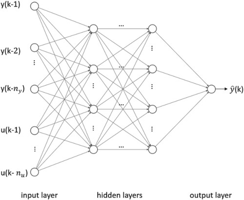
FNN is the neural network topology with no previous states or outputs feedback loop. According to the structure of hidden units, FNN can be generally divided into three types: the multilayer perceptron (MLP)(Acuna et al., 2012; Wang & Song, 2014), the radial basis function network (RBFN) (Ahmed et al., 2010; Moody & Darken, 1988; Pérez-Sánchez et al., 2018) and the temporal convolution neural network (CNN) (Bai et al., 2018; Cao et al., 2021; Fan et al., 2021; Hao et al., 2020; Oord et al., 2016; Tang et al., 2022). FNN can be generally described with the NARX model family, where the system is assumed to have white noise. For simplicity, the single-input and single-output (SISO) model is demonstrated in this paper. The multi-input and multiple-output (MIMO) case, where the variables are all endogenous, is referred to as the nonlinear vector autoregressive (NVAR) model and is usually used for iterative prediction (Gauthier et al., 2021). The SISO NARX model can be described as follows: (1) $\begin{array}{rl}y(k)& =F[y(k-1),y(k-2),\dots ,y(k-n_y),u(k-1),\\ & u(k-2),\dots ,u(k-n_u)]+e(k),\end{array}$(1) where F$[\cdot ]$ can be any nonlinear function and $n_y$, $n_u$ are the maximum time delay of the system output $y$ and exogenous input $u$ respectively. The FNN representing the NARX model is known as the series-parallel mode NARX network (Jumilla-Corral et al., 2021; Wang & Song, 2014). In Figure 1, an example of MLP representing the NARX model is illustrated.

The FNN uses the direct method for prediction. The network output can be either a certain time step ahead value $y(k+n)$ or values over a certain time span $\tau$ ahead $\{y(k+n),y(k+n+1),\dots ,y(k+n+\tau )\}$. As long as the FNN has promising approximation ability, n steps can be long-term (Wei & Billings, 2006). However, when the future input data is not available, only the reclusive method can be applied, which implies that the previous prediction result of the FNN must be used as input to produce a new prediction. Since the FNN is trained with the direct method, as long as the error between system output and model output is not zero, the error will be accumulated as the prediction goes on, ending up with a potentially poor result (Wang & Song, 2014). To overcome this problem, recurrent neural networks (RNNs) have been developed.

Figure 1. The structure of series-parallel mode NARX MLP.

In the RNN, past information is transferred through the previous states or outputs, and each time step shares the same weight, which is similar to the nonlinear state space model. A general nonlinear state-space model in the discrete domain is described as follows (Ljung et al., 2020): (2) $\begin{array}{rl}x(t+1)& =f(x(t),y(t),u(t),\theta )\end{array}$(2) (3) $\begin{array}{rl}\hat{y}(t\mid \theta )& =h(x(t),\theta ),\end{array}$(3) where $x$, $y$ and $u$ are the system state, output, and input respectively. The nonlinear functions $f$ and $h$ can be parametrised by $\theta$ in various ways. In RNNs, the $f$ and $h$ become activation functions and $\theta$ become the weights and biases. An example of vanilla RNN including the previous output feedback (Jordan) type and previous state feedback (Elman) type is shown below: (4) $\begin{array}{rl}{h}_t& ={\sigma }_h(W_{hx}{x}_t+W_{hh}{y}_{t-1}+b_h)\end{array}$(4) (5) $\begin{array}{rl}{h}_t& ={\sigma }_h(W_{hx}{x}_t+W_{hh}{h}_{t-1}+b_h)\end{array}$(5) (6) $\begin{array}{rl}{y}_t& ={\sigma }_y(W_y{h}_t+b_y).\end{array}$(6) The Jordan RNN can be represented by Equations (4(6) $\begin{array}{rl}{y}_t& ={\sigma }_y(W_y{h}_t+b_y).\end{array}$(6) ) and (6). The Elman RNN can be represented by Equations (5) and (6). In Eqs. (4) – (6), the hypermeter ${\sigma }_h$, ${\sigma }_y$ are the activation functions of the hidden layer and output layer, respectively. The parameter $W_{hx}$, $W_{hh}$ $b_h$,$W_y$, $b_y$ are the weights and biases of the hidden layer and output layer, respectively. The values of $h_{t-1}$ and $y_{t-1}$ are the previous state and previous output (Elman, 1990). Modern RNNs such as the long-short term memory (LSTM) and gated recurrent unit (GRU), which were developed based on the Elman RNN by controlling the information flow with gates, can also be regarded as examples of the nonlinear state-space model (Ljung et al., 2020).

RNNs address the reclusive prediction error by training via the backpropagation through time (BPTT) within a selected time window $\tau$ (Werbos, 1990). The BPTT takes the accumulated error into account by updating parameters based on both current prediction errors and future prediction errors within the time window τ in training. Since the accumulated loss is only optimised within τ, the value of τ should be selected the same as or larger than the maximum time delay of the input time series that affects the output. Therefore, the time window is closely related to the system order.

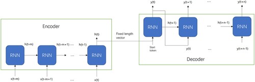
One limitation of the typical recurrent layer is that the time window of its inputs and outputs is required to be fixed during the training. To tackle this problem, the encoder-decoder model, which is also referred as the sequence to sequence (seq2seq) model, is designed for modelling when the memory window of input and output sequence is not fixed (Liu et al., 2021). The typical seq2seq model using RNN as the encoder and decoder is shown in Figure 2. Two separate RNNs are adopted as the encoder and decoder, respectively where the input time window is $m$ and the output time window is $n$. The encoder takes the input sequence and only outputs a fixed-length vector to the decoder, either using the state of the final time step or a temporal embedding vector if the attention mechanism is adopted to tackle the memory loss of the decoder (Bahdanau et al., 2014; Vaswani et al., 2017). The decoder takes the fixed-length vector for initial prediction when a start token is received. The start token can be either one hot vector or a part of time series before the value is predicted (Vaswani et al., 2017; Zhou et al., 2021). It should be noted that both FNN and RNN can be used for the encoder and decoder (Lim & Zohren, 2021). Furthermore, the decoder part can be either autoregressive or non-autoregressive (Vaswani et al., 2017; Zhou et al., 2021). Therefore, the type of parametric model corresponding to an encoder-decoder model is dependent on its specific structure.

Figure 2. Seq2seq model with RNN encoder and decoder expanding along time.

3. Neural network models for system identification

In the paradigm of parametric system identification, the model is built based on observed system inputs and outputs time series. Then the correlation, causality and spectrum analysis, and system behaviour forecast are implemented based on the identified model. When the neural network acts as the model for parametric system identification, the neural network will be trained with the historical system inputs and outputs. Then the analysis and prediction are implemented based on the trained neural network.

The model interpretability and modelling with nonstationary realisations are two challenges of parametric system identification. The interpretability of a model often refers to the model’s transparency to correlation, causality, and spectrum analysis. The system characteristics, including the significant system inputs, system order and delay information, should be revealed through the parametric correlation and causality analysis. For spectrum analysis, the model built in the time domain should be capable of transformation to the frequency domain. However, the original structures of deep neural networks are regarded as black boxes and hard to interpret (Cui & Athey, 2022; Rudin, 2019). Furthermore, for nonstationary time series, conventional neural networks are incapable of tracking data dynamics and adapting to underlying changes (Ditzler et al., 2015). Recently, some research has been conducted to enhance the interpretability of neural networks and their performance in modelling nonstationary time series. Table 1 summarises the research progress in addressing two major challenges of parametric system identification based on different types of neural networks for dynamic system modelling.

Table 1. The capability of different types of neural networks to tackle parametric system identification challenges.

		Interpretability		Nonstationarity
General NN types	Subtypes	Correlation & Causality	Spectrum	Homogeneous nonstationary	Inhomogeneous nonstationary
FNN	MLP	✓	✓
	RBFN	✓		✓	✓
	CNN	✓		✓
RNN	Vanilla RNNs		✓
	Modern RNNs	✓		✓
Encoder – decoder	Autoregressive decoder	✓		✓	✓
	Non-autoregressive decoder			✓	✓

3.1. System characteristic identification

In parametric system identification, the system characteristics, including significant system inputs, system order, delay information, and system spectrum information, are identified based on the interpretation of the parametric model. In Table 2, some milestone works of system characteristic identification using different neural networks are reviewed in terms of their key operations and limitations. The detail of these milestone works and their follow-up works are discussed below.

Table 2. Summary of different types of neural networks in system characteristic identification.

Basic NN type	Key operations	Outcome	Revealed system information	Limitation
MLP (Montalto et al., 2015)	Adopting the NN in the NUE framework. Measure the causality according to relative prediction error.	Nonlinear Granger causality	Significant system inputs	Input time series length (maximum time delay) is fixed. High computational costs.
RBFN (Billings et al., 2007)	Preselecting the centres of kernels with K-means. Heuristically setting kernel width. Selecting significant bases and calculate their weights with FROLS.	Parsimonious Multiscale RBFN structure	System order Specific time delay of input and output	Not fully end-to-end since the pre-processing of kernel centre and width selection is required.
MLP/ Vanilla RNN/ LSTM (Tank et al., 2021)	Adopting component-wise structure to predict each variable separately. LASSO penalty on the weights of the first layer.	Nonlinear Granger causality	Significant system inputs System order (maximum time delay) Inputs specific time delay	The latent confounder problem is not considered.
CNN (Nauta et al., 2019)	Adopting depthwise structure to separate the contribution of inputs to different outputs. Detecting nonlinear correlation between inputs and outputs with thresholded attention. Measure the causality with permutation importance validation	Nonlinear Granger causality	Significant system inputs System order (maximum time delay)	Specific time delays cannot be revealed.
MLP/ Vanilla RNN (Fung et al., 1997)	Approximating activation function with truncated Volterra series	GFRF	System spectrum information	Only applicable with single hidden layer MLP and Jordan RNN.
MLP (Tutunji, 2016)	Approximating activation function with the first two terms of the Taylor series to avoid nonlinearity.	Transfer function	System spectrum information	Only applicable with single hidden layer MLP. Only a linear transfer function can be derived.

3.1.1. The selection of significant system inputs

The first type of method to select significant system inputs is based on the nonlinear Granger causality (GC) test, where a measure is defined to evaluate whether a certain input helps to predict the output. Montalto et al. (2015) proposed an NN-GC approach where the nonlinear GC is derived by calculating the difference between prediction errors of MLP with and without the past information of certain input variables using the non-uniform embedding (NUE) strategy. NUE is the framework to select the most informative lagged input one after another. However, the implementation is complicated with high computational costs. In (Wang et al., 2018), it has been tested that the NUE strategy version of the 20-order NN-GC model costs almost twice as much CPU time as the NN-GC without NUE.

Based on NN-GC, in (Wang et al., 2018), the RNN-GC framework was developed where both linear and nonlinear Granger causalities are derived by calculating the prediction error of LSTM with and without a certain input variable. In comparison to NN-GC (Montalto et al., 2015), which uses MLP as the prediction model, RNN is less prone to overfitting due to its weight sharing over time, which makes the parameter dimension irrelevant to the length of the input time series. This makes RNN-GC less sensitive to the model order, resulting in a higher accuracy of causality detection. Furthermore, since the parameter dimension is irrelevant to the length of the input time series, one fixed RNN structure is able to fit time series with different maximum time delays, which makes it more flexible than MLP (Wang et al., 2018). A similar framework has been implemented in (Rosoł et al., 2022), except that the Wilcoxon signed-rank test is adopted to assess the significance of causality. In (Li et al., 2020), causality is expanded to include the effect of future values on present values, which is detected using a bidirectional LSTM. Recently, Liu et al. (2021) proposed the seq2seq-LSTM Granger Causality (SLGC) framework, where the LSTM-based encoder-decoder model is adopted for prediction. The seq2seq model can be adopted when the length of the input and output sequence is not fixed and equal in training. The nonlinear Granger causality is calculated by comparing the fraction of variance explained by the forecasting model with and without a certain input variable, measured by the R-squared score. However, these methods are relatively more complicated than the following fully end-to-end method.

The sparse regression method is another way to select significant system inputs where the nonlinear GC between inputs and outputs is derived in a fully end-to-end manner. In (Tank et al., 2021), the component-wise LSTM (cLSTM) was developed to disentangle the contribution of different inputs to the outputs. The group least absolute shrinkage and selection operator (LASSO) penalty is applied on all weights in the first cLSTM layer. Both gate weights and cell state weights show the same sparsity pattern indicating the significant inputs. However, only the causality can be detected in cLSTM, while the maximum time delay and specific time delay cannot be derived by the penalty-based method on RNN. Because the weight is allocated for each time step in MLP while the weight of RNN shares over time, there is no way to inspect the contribution of a variable at a certain time step according to the weight of RNN.

Similarly, in (Khanna & Tan, 2019), the causality was derived by applying group LASSO penalty on the economy statistical recurrent unit (eSRU) which is a simplified version of SRU with fewer parameters to make it less susceptible to overfitting. In testing, with the simulation dataset that includes Lorenz-96 and vector autoregression (VAR), the eSRU with LASSO penalty demonstrates almost perfectly recover of the true causality, achieving an Area Under the Receiver Operating Characteristic curve (AUROC) of nearly 93%. This AUROC is more than 10% higher than that of cLSTM. Similarly, for the blood oxygenation level dependent (BOLD) imaging dataset, the eSRU outperforms cLSTM significantly, achieving an additional AUROC of nearly 14%. However, in the DREAM-3 In Silico Network Challenge dataset, the eSRU only exhibits a slight improvement over cLSTM. One limitation of all research mentioned above is that the hidden confounder problem has not been considered.

3.1.2. The identification of system order and specific delay terms

The identification of system order (maximum time delay) and the specific input-output time delay is usually more challenging than the selection of significant system inputs because the delay information should be revealed in the causality analysis. In (Tank et al., 2021), the component-wise MLP (cMLP) is developed to disentangle the contribution of different inputs to the outputs. The nonlinear Granger causality, maximum time delay and specific time delay can be derived by applying the group LASSO, hierarchical LASSO, and group sparse group LASSO penalty on the first hidden layer respectively. However, the hidden confounder problem has not been considered.

In (Billings et al., 2007), the multiscale RBFN was developed to capture the system dynamics. Similar to the derivation of the polynomial NARMAX model with ERR-OLS, the FROLS algorithm is applied to select significant RBF bases and calculate their weights (Billings, 2013; Billings et al., 2007). Since the delay information is contained in RBF bases, the system order and specific input-output delay information can be revealed. However, pre-processing such as clustering is required to determine the centre and width of each node heuristically, which makes it relatively more complicated than the fully end-to-end method.

Nauta et al. (2019) developed the Temporal Causal Discovery Framework (TCDF) to obtain causality while predicting the target time series. In the TCDF, the Attention-based Dilated Depthwise Separable Temporal Convolutional Networks (AD-DSTCNs) was developed to separate the contribution of inputs to different outputs when representing the NVAR model. In AD-DSTCNs, the nonlinear correlation between inputs and outputs is derived by the hard spatial attention which is implemented by setting the threshold on the attention score since the correlation and causality are binary decision problems. Then all the input variables correlated to the output are regarded as potential causes of the output and validated by the permutation importance validation method to find true causes if all confounders are measured. Finally, the maximum time delay (system order) can be discovered by following the path with the highest kernel weights from the output layer back to the input layer thanks to the depthwise separable structure and weight-sharing property of convolution layers. However, the specific time delay cannot be derived since only the path with the highest kernel weights can be tracked.

3.1.3. Spectrum analysis

Similar to the conventional parametric system identification approach (Li & Billings, 2005), the spectrum analysis for the neural networks trained in the time domain is based on model transformation. However, up to now, only single-hidden-layer MLP and RNN can be transferred to a frequency domain model for spectrum analysis. In (Fung et al., 1997), the GFRF of single-hidden-layer MLP and Jordan RNN is derived through truncated Volterra series expansion of the activation function. However, the applications on modern RNNs, such as LSTM and GRU have not been studied. In (Tutunji, 2016), the linear transfer function of the single-hidden-layer MLP whose input includes both system’s historical input and output is derived by approximating the activation function with the first two terms of the Taylor series expansion to avoid nonlinearity. However, the nonlinear GFRF is not derived, which ends up with a steady-state error when the MLP represents nonlinear systems.

3.2. System modelling with nonstationary realisations

There are generally two types of training methods for neural networks, either online or offline, for tracking the data dynamics and adapting to the underlying system changes from nonstationary realisations. The online training method is adopted to adjust the neural networks when the system is chaotic or time-varying generating inhomogeneous nonstationary time series. The offline method is more often employed to train neural networks to learn the trend and seasonality of homogeneous time series. Some milestone works of modelling using neural networks with nonstationary realisations are reviewed and summarised in Table 3 with respect to their training types and key operations.

Table 3. Milestone works of modelling using neural networks with nonstationary realisations.

Nonstationary type	Basic NN type	Training type	Key operations
Homogeneous	RBFN (Chng et al., 1996)	Offline	Taking the difference operation of inputs to decompose trends and seasonality
Homogeneous	Encoder-decoder (Wu et al., 2021)	Offline	Detect period-based dependency with Auto-correlation mechanism Decompose seasonality and trend progressively with a Series decomposition block
Inhomogeneous	RBFN (Chen et al., 2016)	Online	Detect the time to replace the kernel according to the squared relative error Select the kernel to be replaced according to the weighted node-output variance Update parameters with RLS
Inhomogeneous	Encoder-decoder (Du et al., 2021)	Offline	A time series is separated into various homogeneous intervals with a temporal distribution characterisation module. Common knowledge is extracted from various homogeneous intervals by the temporal distribution matching module.
Homogeneous & Inhomogeneous	RBFN (Liu et al., 2020)	Online	Combine the GRBF (Chng et al., 1996) and fast tuneable RBF (Chen et al., 2016)

3.2.1. Homogeneous nonstationary

To address homogeneous nonstationary time series, Wu et al. (2021) proposed the Autoformer to learn the intricated temporal pattern for long-term predictions. In the Autoformer, the auto-correlation mechanism was developed to detect period-based dependency and aggregate corresponding subseries as temporal embeddings. Then, the series decomposition block is designed to decompose seasonality and trend progressively. The encoder only focuses on seasonal part modelling and the decoder predicts the trend and seasonal component with accumulation structure and stacked Auto-Correlation mechanism, respectively. This approach outperformed the self-attention-based model like Informer (Zhou et al., 2021) and Reformer (Kitaev et al., 2020) since the auto-correlation mechanism learns the sub-series dependency while the self-attention mechanism only learns the point-wise dependency (Wu et al., 2021). It also outperformed the neural networks that decompose trend and seasonality in pre-processing, such as the CNN-based DeepGLO (Sen et al., 2019) and MLP-based N-BEATS (Oreshkin et al., 2020). This is because the pre-processing is constrained to historical information while Autoformer progressively decomposes seasonality and trend series throughout the whole forecasting process (Wu et al., 2021). However, due to its complicated and fixed structure, it is non-adaptive to track the time-varying underlying process dynamics in inhomogeneous non-stationary data.

In (Chng et al., 1996), the gradient RBF (GRBF) network was developed, where the input of RBFN becomes a certain order difference operation of the historical data. The order of the difference operation is a hyperparameter that can be tuned to achieve lower loss. The purpose of the difference operation is to mitigate the trend and seasonal effect. When a certain input is close to the centre of a hidden unit, the hidden unit is activated, performing as a localised one-step-ahead prediction of the output. Hence, the GRBF senses a certain order of localised derivative of time series, which captures the trend and seasonal pattern. However, the significant inputs of the actual system cannot be selected in the same manner as (Billings et al., 2007) since the input of GRBF is a certain order difference of data instead of the data from the original measurement space. Although the fixed structure makes it non-adaptive to underlying changes in inhomogeneous nonstationary realisations, the shallow structure of RBF allows it to be adjusted to be adaptable (Liu et al., 2020).

3.2.2. Inhomogeneous nonstationary

For the inhomogeneous nonstationary time series, the actual system may be time-varying or suffering from different disturbances. Some traditional methods like RLS can be used to adaptively estimate the weight of RBFN online (Chen, 1995). For simplicity, a large number of training data can be randomly selected as kernel centres, and then RLS can be applied to estimate the weight, which is known as the online sequential extreme learning machine (OS-ELM) (Wang & Han, 2014). However, adaptively learning the weight of the fixed structure of RBFN is not expressive enough when the significant inputs and causal relationship are time-varying (Liu et al., 2020). The fast-tuneable RBF was developed to adaptively learn the network structure and parameters. The node will be replaced when the squared relative error (SRE) is larger than a user-set threshold. The node with the least contribution measured by weighted node-output variance (WNV) will be abandoned. One simple way to set new node centre and width is using the current input data and the new maximum distance between centres, respectively. Then the weight can be updated with gradient descent or least squares. If no node is replaced, parameters will just be updated by RLS (Chen et al., 2016). However, the fast-tuneable RBF doesn’t take the homogeneous nonstationary condition into account.

Inspired by the conventional sliding-window model structure selection approach, Du et al. (2021) proposed an adaptive RNNs (AdaRNN) framework to identify different phases and fitted one robust model capturing the common knowledge shared among different periods. In AdaRNN, the target time series are split into $K$ most dissimilar segments by reclusively maximising the distance between distributions of the randomly selected period with the greedy algorithm in the Temporal Distribution Characterisation (TDC) module. Then each segment is regarded as a homogeneous interval. Finally, an RNN-based encoder-decoder model is adopted to robustly fit all selected phases by matching distributions between RNN states from different phases to extract common knowledge in the encoder with the Temporal Distribution Matching (TDM) module. However, the end-to-end optimisation of both TDC and TDM remains a problem. Furthermore, the adaptive parameter learning methods have not been considered, which makes it hard to track some rapid changes in the time series generated by a time-varying system.

Recently, Liu et al. (2020) combined the GRBF and the fast tuneable RBF creating the fast adaptive GRBF networks which is capable of identifying the system with data that is both homogeneous and inhomogeneous nonstationary. However, it still suffers from the same problem as the GRBF that the significant inputs of the actual system cannot be selected.

4. Research gaps and future direction

Many processes in climate systems and neuro systems are inherently nonstationary, which makes the system characteristics identification challenging (He & Yang, 2021; Zhao et al., 2016). In conventional parametric system identification approaches, a robust and adaptive parsimonious model, such as the time-varying NARMAX (TV-NARMAX), can be derived with nonstationary realisations. The system input-output delay information can be revealed in the model structure and the spectrum information can be revealed by transferring the TV-NARMAX model in the time domain to a time-varying GFRF (TV-GFRF) (He et al., 2013, 2015; Li et al., 2017) in the frequency domain. The significant inputs can be derived by the windowed ERR-based causality test (Zhao et al., 2012, 2017). Although a lot of studies have been carried out to either improve the interpretability of neural networks in the stationary scenario or their prediction performance with nonstationary realisations, the system characteristics identification with nonstationary realisations based on neural networks is overlooked, which potentially attracts future research. Although some state-of-the-art (SOTA) neural networks, such as Autoformer and AdaRNN, have been developed, there has been very limited research on long-term forecasting with both homogeneous and inhomogeneous realisations. A potential future research direction could be merging the TDC and TDM mechanisms from AdaRNN into the Autoformer to enhance its adaptability.

In conventional parametric system identification, the residual analysis is critical for model validation during a homogenous interval. Whether the residual is white noise indicates if all useful information in both input and output time series has been fully extracted by the model. If the residual is autocorrelated, the model is biased. Furthermore, if the residual is correlated with the explanatory variables, a condition known as endogeneity, the model is also biased (Box et al., 2015). Noise modelling should usually be considered to create unbiased estimation (Billings, 2013). On the other hand, if the residual has zero mean but its variance is always changing, a condition known as heteroscedasticity, the model is unbiased but the confidence intervals and hypotheses tests cannot be relied on. Then some models should also be built to estimate the change of variance (Bodhanwala, 2014; Box et al., 2015). Most of the validation and testing of neural networks in previous research is only based on prediction errors, while the residual analysis has not been considered. The question of whether the produced neural network is unbiased and has valid confidence intervals is often neglected, but it is important in parametric system identification. Although the residual analysis is considered in (Ljung et al., 2020), noise modelling and variance estimation with neural networks remain a problem. Therefore, it is still difficult to build an unbiased neural network model when the noise is coloured and correlated with system inputs and outputs. Future research is required to address this bottleneck to further promote neural networks in system identification.

5. Conclusions

This paper reviewed recent studies on parametric system identification based on three types of neural networks, including feedforward neural networks, recurrent neural networks and encoder-decoder, which have better approximation ability and rely less on prior knowledge than conventional approaches. It has been discovered that the FNNs and RNNs can be regarded as NARX and nonlinear state-space models, respectively, while the parametric model corresponding to an encoder-decoder depends on its specific structure. In system characteristic identification based on the interpretation of neural networks, it is observed that more research has been conducted on selecting significant inputs and extracting input-output delay information, whereas the spectrum analysis with neural networks has been relatively less studied and presents an area for future research. On the other hand, system modelling with both homogeneous and inhomogeneous realisations have been less studied, leaving a gap for future research. Furthermore, long-term forecasting with both homogeneous and inhomogeneous realisations could be potentially handled by leveraging the advantages of multiple SOTA neural networks, such as Autoformer and AdaRNN. Finally, it was identified that system characteristics identification with nonstationary realisations and modelling with coloured noise based on neural networks remain understudied and waiting to be explored.

Data sharing statement

Here is no data available for this article.

Disclosure statement

No potential conflict of interest was reported by the author(s).

Additional information

Notes on contributors

Aoxiang Dong

Aoxiang Dong graduated from Newcastle University with Distinction in Automation and Control in 2019. While studying at Newcastle University, he focused on designing digital control systems with advanced control theory and stochastic state estimation. He is currently pursuing a PhD in nonlinear system identification for data-driven control and decision-making.

Andrew Starr

Andrew Starr is a Professor of Maintenance Systems, Head of TES Institute and Director of Education in the School of Aerospace, Transportation and Manufacturing at Cranfield University. His works in novel sensing, e-maintenance systems, and decision-making strategies has been recognised as internationally excellent.

Yifan Zhao

Yifan Zhao was born in Zhejiang, China. He received a Ph.D. degree in Automatic Control and System Engineering from the University of Sheffield, Sheffield, UK, in 2007. He is currently the Professor of Data Science at Cranfield University, Cranfield, UK. His research interests include computer vision, signal processing, non-destructive testing, active thermography, and nonlinear system identification.

References

- Acuna, G., Ramirez, C., & Curilem, M. (2012). Comparing NARX and NARMAX models using ANN and SVM for cash demand forecasting for ATM. Proceedings of the international joint conference on neural networks. https://doi.org/10.1109/IJCNN.2012.6252476
- Aggarwal, C. C. (2018). Neural networks and deep learning. Springer, 10(978), 3. https://doi.org/10.1007/978-3-319-94463-0
- Ahmed, N. K., Atiya, A. F., el Gayar, N., & El-Shishiny, H. (2010). An empirical comparison of machine learning models for time series forecasting. Econometric Reviews, 29(5), 594–621. https://doi.org/10.1080/07474938.2010.481556
- Ardalani-Farsa, M., & Zolfaghari, S. (2010). Chaotic time series prediction with residual analysis method using hybrid elman–NARX neural networks. Neurocomputing, 73(13–15), 2540–2553. https://doi.org/10.1016/j.neucom.2010.06.004
- Bahdanau, D., Cho, K. H., & Bengio, Y. (2014). Neural machine translation by jointly learning to align and translate. 3rd International conference on learning representations, ICLR 2015 - Conference Track Proceedings. https://arxiv.org/abs/1409.0473v7.
- Bai, S., Kolter, J. Z., & Koltun, V. (2018). An empirical evaluation of generic convolutional and recurrent networks for sequence modeling. http://arxiv.org/abs/1803.01271.
- Billings, S. A. (2013). Introduction. In Nonlinear system identification: NARMAX methods in the time, frequency, and spatio-temporal domains (pp. 1–14). John Wiley & Sons, Ltd. https://doi.org/10.1002/9781118535561
- Billings, S. A., Wei, H.-L., & Balikhin, M. A. (2007). Generalized multiscale radial basis function networks. Neural Networks, 20(10), 1081–1094. https://doi.org/10.1016/j.neunet.2007.09.017
- Bodhanwala, M. (2014). A novel non-linear GARCH framework for modelling the volatility of heteroskedastic time series. PhD Thesis, University of Sheffield.
- Box, G. E. P., Jenkins, G. M., Reinsel, G. C., & Ljung, G. M. (2015). Time series analysis : Forecasting and control (5th ed.).
- Brunton, S. L., Proctor, J. L., & Kutz, J. N. (2016). Discovering governing equations from data by sparse identification of nonlinear dynamical systems. Proceedings of the National Academy of Sciences, 113(15), 3932–3937. https://doi.org/10.1073/pnas.1517384113
- Cao, Y., Ding, Y., Jia, M., & Tian, R. (2021). A novel temporal convolutional network with residual self-attention mechanism for remaining useful life prediction of rolling bearings. Reliability Engineering and System Safety, 215, https://doi.org/10.1016/J.RESS.2021.107813
- Chen, H., Gong, Y., Hong, X., & Chen, S. (2016). A fast adaptive tunable RBF network for nonstationary systems. IEEE Transactions on Cybernetics, 46(12), 2683–2692. https://doi.org/10.1109/TCYB.2015.2484378
- Chen, S. (1995). Nonlinear time series modelling and prediction using Gaussian RBF networks with enhanced clustering and RLS learning. Electronics Letters, 31(2), 117–118. https://doi.org/10.1049/el:19950085
- Chng, E. S., Chen, S., & Mulgrew, B. (1996). Gradient radial basis function networks for nonlinear and nonstationary time series prediction. IEEE Transactions on Neural Networks, 7(1), 190–194. https://doi.org/10.1109/72.478403
- Cui, P., & Athey, S. (2022). Stable learning establishes some common ground between causal inference and machine learning. Nature Machine Intelligence, 4(2), 110–115. https://doi.org/10.1038/s42256-022-00445-z
- Ditzler, G., Roveri, M., Alippi, C., & Polikar, R. (2015). Learning in nonstationary environments: A survey. IEEE Computational Intelligence Magazine, 10(4), 12–25. https://doi.org/10.1109/MCI.2015.2471196
- Du, Y., Wang, J., Feng, W., Pan, S., Qin, T., Xu, R., & Wang, C. (2021). AdaRNN: Adaptive learning and forecasting of time series. Proceedings of the 30th ACM International conference on information & knowledge management, 402–411. https://doi.org/10.1145/3459637.3482315.
- Elman, J. L. (1990). Finding structure in time. Cognitive Science, 14(2), 179–211. https://doi.org/10.1207/s15516709cog1402_1
- Fan, J., Zhang, K., Huang, Y., Zhu, Y., & Chen, B. (2021). Parallel spatio-temporal attention-based TCN for multivariate time series prediction. Neural Computing and Applications, 1–10. https://doi.org/10.1007/S00521-021-05958-Z/FIGURES/7
- Fung, C. F., Billings, S. A., & Zhang, H. (1997). Generalised transfer functions of neural networks. Mechanical Systems and Signal Processing, 11(6), 843–868. https://doi.org/10.1006/mssp.1997.0112
- Gauthier, D. J., Bollt, E., Griffith, A., & Barbosa, W. A. S. (2021). Next generation reservoir computing. Nature Communications, 12(1), 1–8. https://doi.org/10.1038/s41467-021-25801-2
- Goodfellow, I., Bengio, Y., & Courville, A. (2016). Deep learning. MIT Press.
- Gu, Y., Wei, H. L., Boynton, R. J., Walker, S. N., & Balikhin, M. A. (2019). System identification and data-driven forecasting of AE index and prediction uncertainty analysis using a new cloud-NARX model. Journal of Geophysical Research: Space Physics, 124(1), 248–263. https://doi.org/10.1029/2018JA025957
- Hao, H., Wang, Y., Xia, Y., Zhao, J., & Shen, F. (2020). Temporal convolutional attention-based network for sequence modeling. https://arxiv.org/abs/2002.12530v2.
- He, F., Billings, S. A., Wei, H. L., Sarrigiannis, P. G., & Zhao, Y. (2013). Spectral analysis for nonstationary and nonlinear systems: A discrete-time-model-based approach. IEEE Transactions on Bio-Medical Engineering, 60(8), 2233–2241. https://doi.org/10.1109/TBME.2013.2252347
- He, F., Wei, H.-L., & Billings, S. A. (2015). Identification and frequency domain analysis of non-stationary and nonlinear systems using time-varying NARMAX models. International Journal of Systems Science, 46(11), 2087–2100. https://doi.org/10.1080/00207721.2013.860202
- He, F., & Yang, Y. (2021). Nonlinear system identification of neural systems from neurophysiological signals. Neuroscience, 458, 213–228. https://doi.org/10.1016/j.neuroscience.2020.12.001
- Hong, X., Mitchell, R. J., Chen, S., Harris, C. J., Li, K., & Irwin, G. W. (2008). Model selection approaches for non-linear system identification: A review. International Journal of Systems Science, 39(10), 925–946. https://doi.org/10.1080/00207720802083018
- Hornik, K., Stinchcombe, M., & White, H. (1989). Multilayer feedforward networks are universal approximators. Neural Networks, 2(5), 359–366. https://doi.org/10.1016/0893-6080(89)90020-8
- Jiao, H., Zhang, L., Shen, Q., Zhu, J., & Shi, P. (2018). Robust gene circuit control design for time-delayed genetic regulatory networks without SUM regulatory logic. https://doi.org/10.1109/TCBB.2018.2825445.
- Jumilla-Corral, A. A., Perez-Tello, C., Campbell-Ramírez, H. E., Medrano-Hurtado, Z. Y., Mayorga-Ortiz, P., & Avitia, R. L. (2021). Modeling of harmonic current in electrical grids with photovoltaic power integration using a nonlinear autoregressive with external input neural networks. Energies, 14(13), 4015. https://doi.org/10.3390/EN14134015.
- Kaiser, E., Kutz, J. N., & Brunton, S. L. (2018). Sparse identification of nonlinear dynamics for model predictive control in the low-data limit. Proceedings of the Royal Society A, 474(2219), https://doi.org/10.1098/RSPA.2018.0335
- Khanna, S., & Tan, V. Y. F. (2019). Economy statistical recurrent units for inferring nonlinear granger causality. https://arxiv.org/abs/1911.09879v2.
- Kitaev, N., Kaiser, Ł, & Levskaya, A. (2020). Reformer: The efficient transformer. ICLR. http://arxiv.org/abs/2001.04451.
- Li, L. M., & Billings, S. A. (2005). Discrete time subharmonic modelling and analysis. International Journal of Control, 78(16), 1265–1284. https://doi.org/10.1080/00207170500293594
- Li, T., Li, G., Xue, T., & Zhang, J. (2020). Analyzing brain connectivity in the mutual regulation of emotion – movement using bidirectional granger causality. Frontiers in Neuroscience, 14, 369. https://doi.org/10.3389/fnins.2020.00369
- Li, Y., Cui, W.-G., Guo, Y.-Z., Huang, T., Yang, X.-F., & Wei, H.-L. (2017). Time-varying system identification using an ultra-orthogonal forward regression and multiwavelet basis functions with applications to Eeg. IEEE Transactions on Neural Networks and Learning Systems, 1–13. https://doi.org/10.1109/TNNLS.2017.2709910
- Li, Y., Wei, H. L., Billings, S. A., & Sarrigiannis, P. G. (2016). Identification of nonlinear time-varying systems using an online sliding-window and common model structure selection (CMSS) approach with applications to EEG. International Journal of Systems Science, 47(11), 2671–2681. https://doi.org/10.1080/00207721.2015.1014448
- Lim, B., & Zohren, S. (2021). Time-series forecasting with deep learning: A survey. Philosophical Transactions of the Royal Society A, 379(2194), 20200209. https://doi.org/10.1098/rsta.2020.0209
- Liu, B., He, X., Song, M., Li, J., Qu, G., Lang, J., & Gu, R. (2021). A method for mining granger causality relationship on atmospheric visibility. ACM Transactions on Knowledge Discovery from Data (TKDD), 15(5), https://doi.org/10.1145/3447681
- Liu, T., Chen, S., Liang, S., Du, D., & Harris, C. J. (2020). Fast tunable gradient RBF networks for online modeling of nonlinear and nonstationary dynamic processes. Journal of Process Control, 93, 53–65. https://doi.org/10.1016/j.jprocont.2020.07.009
- Liu, T., Chen, S., Liang, S., Gan, S., & Harris, C. J. (2020). Fast adaptive gradient RBF networks for online learning of nonstationary time series. IEEE Transactions on Signal Processing, 68, 2015–2030. https://doi.org/10.1109/TSP.2020.2981197
- Ljung, L., Andersson, C., Tiels, K., & Schön, T. B. (2020). Deep learning and system identification. IFAC-PapersOnLine, 53(2), 1175–1181. https://doi.org/10.1016/j.ifacol.2020.12.1329
- Montalto, A., Stramaglia, S., Faes, L., Tessitore, G., Prevete, R., & Marinazzo, D. (2015). Neural networks with non-uniform embedding and explicit validation phase to assess Granger causality. Neural Networks, 71, 159–171. https://doi.org/10.1016/j.neunet.2015.08.003
- Moody, J., & Darken, C. (1988). Learning with localized receptive fields.
- Nauta, M., Bucur, D., & Seifert, C. (2019). Causal discovery with attention-based convolutional neural networks. Machine Learning and Knowledge Extraction, 1(1), 312–340. https://doi.org/10.3390/MAKE1010019
- Neshat, N., Hadian, H., & Behzad, M. (2018). Nonlinear ARIMAX model for long – term sectoral demand forecasting. Management Science Letters, 8(6), 581–592. https://doi.org/10.5267/j.msl.2018.4.032
- Oord, A. van den, Dieleman, S., Zen, H., Simonyan, K., Vinyals, O., Graves, A., Kalchbrenner, N., Senior, A., & Kavukcuoglu, K. (2016). WaveNet: A generative model for raw audio. ArXiv Preprint, ArXiv:1609.03499. http://arxiv.org/abs/1609.03499.
- Oreshkin, B. N., Carpov, D., Chapados, N., & Bengio, Y. (2020, May 24). N-BEATS: Neural basis expansion analysis for interpretable time series forecasting. ICLR. http://arxiv.org/abs/1905.10437.
- Pérez-Sánchez, B., Fontenla-Romero, O., & Guijarro-Berdiñas, B. (2018). A review of adaptive online learning for artificial neural networks. Artificial Intelligence Review, 49(2), 281–299. https://doi.org/10.1007/s10462-016-9526-2
- Rosoł, M., Młyńczak, M., & Cybulski, G. (2022). Granger causality test with nonlinear neural-network-based methods: Python package and simulation study. Computer Methods and Programs in Biomedicine, 106669, https://doi.org/10.1016/J.CMPB.2022.106669
- Rudin, C. (2019). Stop explaining black box machine learning models for high stakes decisions and use interpretable models instead. Nature Machine Intelligence, 1(5), 206–215. https://doi.org/10.1038/s42256-019-0048-x
- Schön, T. B., Lindsten, F., Dahlin, J., Wågberg, J., Naesseth, C. A., Svensson, A., & Dai, L. (2015). Sequential Monte Carlo methods for system identification. IFAC-PapersOnLine, 48(28), 775–786. https://doi.org/10.1016/j.ifacol.2015.12.224
- Sen, R., Yu, H. F., & Dhillon, I. (2019). Think globally, act locally: A deep neural network approach to high-dimensional time series forecasting. Advances in Neural Information Processing Systems, 32), https://doi.org/10.48550/arxiv.1905.03806
- Shen, Q., Shi, P., Agarwal, R. K., & Shi, Y. (2021). Adaptive neural network-based filter design for nonlinear systems with multiple constraints. IEEE Transactions on Neural Networks and Learning Systems, 32(7), 3256–3261. https://doi.org/10.1109/TNNLS.2020.3009391
- Shen, Q., Shi, P., Zhu, J., Wang, S., & Shi, Y. (2020). Neural networks-based distributed adaptive control of nonlinear multiagent systems. IEEE Transactions on Neural Networks and Learning Systems, 31(3), 1010–1021. https://doi.org/10.1109/TNNLS.2019.2915376
- Tang, P., Du, P., Xia, J., Zhang, P., & Zhang, W. (2022). Channel attention-based temporal convolutional network for satellite image time series classification. IEEE Geoscience and Remote Sensing Letters, 19, https://doi.org/10.1109/LGRS.2021.3095505
- Tank, A., Covert, I., Foti, N., Shojaie, A., & Fox, E. B. (2021). Neural granger causality. IEEE Transactions on Pattern Analysis and Machine Intelligence, 1–1. https://doi.org/10.1109/TPAMI.2021.3065601
- Tutunji, T. A. (2016). Parametric system identification using neural networks. Applied Soft Computing, 47, 251–261. https://doi.org/10.1016/j.asoc.2016.05.012
- Vaswani, A., Brain, G., Shazeer, N., Parmar, N., Uszkoreit, J., Jones, L., Gomez, A. N., Kaiser, Ł, & Polosukhin, I. (2017). Attention is all you need. Advances in Neural Information Processing Systems, 30. https://doi.org/10.48550/arXiv.1706.03762
- Wang, H., & Song, G. (2014). Innovative NARX recurrent neural network model for ultra-thin shape memory alloy wire. Neurocomputing, 134, 289–295. https://doi.org/10.1016/j.neucom.2013.09.050
- Wang, X., & Han, M. (2014). Online sequential extreme learning machine with kernels for nonstationary time series prediction. Neurocomputing, 145, 90–97. https://doi.org/10.1016/j.neucom.2014.05.068
- Wang, Y., Lin, K., Qi, Y., Lian, Q., Feng, S., Wu, Z., & Pan, G. (2018). Estimating brain connectivity with varying-length time lags using a recurrent neural network. IEEE Transactions on Biomedical Engineering, 65(9), 1953–1963. https://doi.org/10.1109/TBME.2018.2842769
- Wei, H. L., & Billings, S. A. (2006). Long term prediction of non-linear time series using multiresolution wavelet models. International Journal of Control, 79(6), 569–580. https://doi.org/10.1080/00207170600621447
- Wei, H. L., & Billings, S. A. (2007). Feature subset selection and ranking for data dimensionality reduction. IEEE Transactions on Pattern Analysis and Machine Intelligence, 29(1), 162–166. https://doi.org/10.1109/TPAMI.2007.250607
- Werbos, P. J. (1990). Backpropagation through time: What it does and how to do it. Proceedings of the IEEE, 78(10), 1550–1560. https://doi.org/10.1109/5.58337
- Wu, H., Xu, J., Wang, J., & Long, M. (2021). Autoformer: Decomposition transformers with auto-correlation for long-Term series forecasting. 35th Conference on Neural Information Processing Systems (NeurIPS). http://arxiv.org/abs/2106.13008.
- Zhao, Y., Bigg, G. R., Billings, S. A., Hanna, E., Sole, A. J., Wei, H. L., Kadirkamanathan, V., & Wilton, D. J. (2016). Inferring the variation of climatic and glaciological contributions to West Greenland iceberg discharge in the twentieth century. Cold Regions Science and Technology, 121, 167–178. https://doi.org/10.1016/j.coldregions.2015.08.006
- Zhao, Y., Billings, S. A., Wei, H., He, F., & Sarrigiannis, P. G. (2013). A new NARX-based Granger linear and nonlinear casual influence detection method with applications to EEG data. Journal of Neuroscience Methods, 212(1), 79–86. https://doi.org/10.1016/j.jneumeth.2012.09.019
- Zhao, Y., Billings, S. A., Wei, H., & Sarrigiannis, P. G. (2012). Tracking time-varying causality and directionality of information flow using an error reduction ratio test with applications to electroencephalography data. Physical Review E, 86(5), 051919. https://doi.org/10.1103/PhysRevE.86.051919
- Zhao, Y., Hanna, E., Bigg, G. R., & Zhao, Y. (2017). Tracking nonlinear correlation for complex dynamic systems using a windowed error reduction ratio method. Complexity, 2017, https://doi.org/10.1155/2017/8570720
- Zhou, H., Zhang, S., Peng, J., Zhang, S., Li, J., Xiong, H., & Zhang, W. (2021). Informer: Beyond efficient transformer for long sequence time-series forecasting. Proceedings of the AAAI Conference on Artificial Intelligence, 35(12), 11106–11115. https://ojs.aaai.org/index.php/AAAI/article/view/17325.
- Zhu, Y.-P., Yuan, J., Lang, Z. Q., Schwingshackl, C. W., Salles, L., & Kadirkamanathan, V. (2021). The data-driven surrogate model-based dynamic design of aeroengine fan systems. Journal of Engineering for Gas Turbines and Power, 143(10), https://doi.org/10.1115/1.4049504