Building Resilience through Social Protection: Evidence from Malawi

Abstract

We apply a well-known resilience index developed by the FAO to data from a cash transfer evaluation in Malawi to address two key questions: Is the FAO index a valid measure of resilience? Can an unconditional cash transfer significantly boost household resilience? Our answer to both these questions is affirmative. The resilience index positively predicts future positive coping behaviour among households (predictive validity) and is a stronger predictor of future coping than consumption or assets. We then find that the unconditional cash transfer increased the resilience index by 12 points, or 30 per cent over the baseline mean index value. Results imply that small, regular, predictable cash transfer payments to ultra-poor households not only protect current consumption but can also build resilience and protect against future shocks.

Keywords:

• Resilience
• cash transfer
• social protection
• food security
• Malawi

JEL CLASSIFICATION CODES:

• I38
• Q18
• O13

1. Introduction

The concept of Resilience has become increasingly popular within the international development community as a framework for profiling and ranking households in terms of their response capacity to shocks and stressors to livelihoods, particularly those that threaten food security. Though relatively new in development economics, the term has a long history of use in mental health studies where resilience is defined as ‘the ability to withstand and rebound from disruptive life challenges’ (Walsh, 2003). In the development literature, resilience is typically discussed in relation to threats to livelihoods and the ability to overcome these threats. The Resilience Alliance, for example, defines resilience as ‘The capacity of a system to absorb disturbance and reorganise while undergoing change’ (Resilience Alliance, 2002), while the Food Security Information Network’s Resilience Measurement Technical Working Group [FSIN-RMTWG] defines resilience as ‘…the capacity that ensures adverse stressors and shocks do not have long-lasting adverse development consequences’ (FSIN-RMTWG, 2014). Barrett and Constas (2014) have proposed a theory of resilience for use in international development that builds on the concept of poverty traps and define resilience as ‘the capacity over time of a person, household or other aggregate unit to avoid poverty in the face of various stressors and in the wake of myriad shocks. If and only if that capacity is and remains high over time, then the unit is resilient’.

The common thread through these and other definitions is the notion that resiliency reflects an ability to successfully avoid poverty and food insecurity even in the event of negative shocks or stressors to an established pattern of livelihood. Resilience does not reflect the elimination of vulnerability to shock or stressors, but the capacity to bounce back when the shocks and stressors do occur. As such, unlike static measures of well-being, such as consumption or assets, behaviour is an important dimension of resilience that makes it unique from a measurement standpoint. Resilience has become particularly relevant in international development due to the increasing disruption in food supplies and agricultural productivity caused by climate change, soil quality depletion due to intensified land use, as well as sporadic incidence of civil unrest and armed conflict.

The empirical literature on resilience in economic development is still relatively recent, and there is not yet a consensus on the ideal approach to measuring resilience nor any validation of alternative measurement approaches (Bahadur, Ibrahim, & Tanner, 2013; Winderl, 2014). Some studies use an indicator of food security or diet diversity as the key outcome or result of higher resilience, and resilience itself is captured through a set of variables representing sources of livelihood and exposure to shocks (CRS, 2013; Frankenberger, Mueller, Spangler, & Alexander, 2013). Two theory based empirical approaches to resilience measurement have been developed to date which hold promise in terms of pushing the methodological frontier in this burgeoning field. Cisse and Barrett (2018) apply the theory of poverty-traps to resilience and estimate a welfare function for pastoralist households in Northern Kenya based on the evolution of livestock holdings over a five-year period. Their method allows previous accumulation of livestock to affect future holdings in a non-linear way to generate the classic S-shaped welfare curve. Estimates of the first and second moments of the welfare distribution for each household are used to generate household specific distributions, which allows the calculation of the probability of the household ending up above a normative cut-off. This probability is the resilience measure, higher values indicating a higher probability of reaching the normative cut-off.

The second approach has been developed by the FAO through the FSIN-RMTWG (FSIN-RMTWG, 2014). In their Resilience Index Measurement and Analysis (RIMA) approach, resilience is conceptualized as a multidimensional latent variable with four key contributing pillars. Indicators within each pillar are combined using structural equations to create a single summary index of resilience capacity. This index can then be used to rank households from most to least resilient for targeting purposes (FAO, 2016). Determinants of resilience capacity at the household and community level can also be investigated to understand which factors contribute to improved resilience, although this is challenging because the obvious factors determining resilience are already used to build the capacity index (Alinovi, D’Errico, Main, & Romano, 2010). Nonetheless, the RIMA approach remains one of the most widely used methodological approaches to resilience measurement (D’Errico, Garbero, Letta, & Winters, 2020).

In this paper we make several new contributions to the literature on resilience using unique data from a randomized control trial (RCT) implemented to evaluate the Government of Malawi’s Social Cash Transfer Program (SCTP). First, we use these data and the RIMA approach to build a multidimensional resilience capacity index (RCI) for households in our sample, all of whom are ultra-poor. We then provide the first formal validation of the RIMA approach by exploiting the panel aspect of our data to see if households with higher resilience capacity at baseline are more likely to adopt positive coping strategies in the future in response to shocks. A valid index would have predictive ability in the sense that it would correctly predict resilient behaviour in the future. We find that the RCI developed based on RIMA approach does indeed have predictive power – 62 per cent of households scoring in the highest quintile of the capacity index at baseline adopted positive coping strategies when faced with a shock in the future, compared to just 25 per cent of households from the bottom quintile of the resiliency index. Future food security is also significantly higher among households in the top quintile of the resilience score at baseline, compared to those in the bottom quintile. These predictive effects are based on the panel of comparison households not exposed to the cash transfer intervention.

Having established the predictive validity of the RCI, we then evaluate the impact of the cash transfer program on resiliency using the RCI as the outcome and controlling for baseline levels of the RCI through a difference-in-difference estimation. We find that the unconditional cash transfer program has a large and statistically significant effect on resiliency, with an effect size in the full sample of 30 per cent of the baseline RCI value. These impacts are almost twice as large for the poorest households at baseline – who are also the least resilient. Key drivers for the increase in the RCI are increased income diversification, increased asset holdings (agricultural tools and livestock), and increased household food production. These results build on similar work that uses the RCI to show that the Lesotho Child Grant Program significantly increases resilience capacity (D’Errico et al., 2020).

Our results have two important implications for the literature on social protection and resilience. A recent position paper by the FAO argues that social protection can be a key programmatic strategy for building resilience in both fragile and stable settings (Winder Rossi, Spano, Sabates-Wheeler, & Kohnstamm, 2017) but the direct evidence of the impact of social protection interventions specifically on resiliency per se is essentially non-existent with the exception of D’Errico et al. (2020). Many studies have looked at the effect of development interventions, including social protection interventions, such as cash transfers on outcomes that are related to or affected by resiliency, such as food security (Bhalla, Handa, Angeles, & Seidenfeld, 2016; Hjelm, Mathiassen, & Wadhhwa, 2016), coping strategies (CRS, 2013) and livelihoods (Handa, Natali, Seidenfeld, Tembo, & Davis, 2018). We provide just the second known rigorous assessment (after D’Errico et al., 2020) of the proposition that social protection can build resiliency, using the case of the Malawi SCTP, which is part of the government’s long-term poverty eradication policy, and using a theory-based approach to measure resilience.

Of particular interest is the fact that the social protection program is an unconditional cash transfer whose primary objective is food security, yet the program has large impacts on assets, livelihoods and other dimensions that strengthen the capacity to withstand a shock—an important component of resiliency. In other words, a program whose primary objective is protection strengthens resiliency by affecting longer-term features of the household that contribute to building resiliency – a potentially important spillover effect. Our paper is the first to provide a (predictive) validity check of the RIMA approach and the corresponding RCI. That the RCI is predictive of future resilient behaviour, at least in the context of this study, suggests that along with the measure developed by Cisse and Barrett (2018) this is a potentially valid measurement tool for future empirical work on resiliency in low-income settings.

The remainder of the paper is organized as follows. Section 2 provides an overview of the Malawi SCTP programme and the evaluation design. Section 3 discusses the RIMA approach and the adaptations to the SCTP data, while Section 4 describes the SCTP data, balance and attrition. Section 5 presents the empirical results on the RCI estimation, predictive validity and programme impacts on the RCI. Section 6 provides a discussion and conclusions.

2. Overview of the Malawi SCTP programme and evaluation design

2.1. Program overview

The SCTP, locally known as the Mtukula Pakhomo, is an unconditional cash transfer programme targeted to ultra-poor, labour-constrained households. The programme began as a pilot in 2006 and has slowly expanded over the years and reaching all 28 districts in the country as off 2021. The objectives of the SCTP are to reduce poverty and hunger, and to increase school enrolment rates among children. The program is implemented by the Ministry of Gender, Children, Disability and Social Welfare (MoGCDSW) with additional policy oversight provided by the Ministry of Finance, Economic Planning and Development (MoFEPD).

Eligibility criteria are based on a household being ultra-poor (unable to meet the most basic urgent needs, including food and essential non-food items, such as soap and clothing) and labour-constrained (defined as having no member ‘fit to work’ or having the ratio of ‘not fit to work’ to ‘fit to work’ of more than three). Household members are defined as ‘unfit to work’ if they are below 19 or above 64 years of age, or if they are aged 19–64 but have a chronic illness or disability, or are otherwise unable to work (Ayala Consulting, 2012). Beneficiary selection is done through a community-based approach with oversight provided by the local District Commissioner’s (DC’s) Office and the District Social Welfare Office (DSWO). Community members are appointed to the Community Social Support Committee (CSSC), and the CSSC is responsible for identifying households that meet these criteria and creating a list. The ultra-poor eligibility condition is verified through a proxy means test (PMT) that is done centrally. Coverage is ∼10 per cent of the household population in each village cluster (VC).

The transfer amount varies based on household size and there is a ‘schooling bonus’ determined by the number of children in the household of primary- or secondary-school age. Transfer amounts remained fixed between 2013 and May 2015 and were adjusted after May 2015 to maintain the real value of the transfer (Table 1). The schooling bonus is not conditional on actual school enrolment but is rather intended to ‘motivate’ households to send children to school. To put these amounts in perspective, on average, the total annual transfer amount received by households was MWK25,622 (US$67) and the average monthly per capita value of the transfer was MWK 559 (US$1.50). Using baseline data, we estimate that the transfer represented 20 per cent of baseline consumption among all beneficiaries.

Table 1. Structure and level of transfers (current MWK)

	2013 to May 2015	After May 2015
1 Member	1,000	1,700
2 Members	1,500	2,200
3 Members	1,950	2,900
4+ Members	2,400	3,700
Each primary school child^a	300	500
Each secondary school member^b	600	1,000

^aProvided for household residents of primary school age.

^bProvided for household residents of secondary-school age.

Additional details of the implementation and operational performance of the SCTP can be found in the main impact evaluation report (CPC, 2016). In particular, there was high adherence in terms of disbursement with up to 99 per cent of target beneficiaries receiving payments as expected and the quantum of money received was also consistent with the schedule in Table 1. Overall impacts of the SCTP based on these data show significant impacts across a wide range of domains including food security and consumption, livestock holdings, and school enrolment of children (Handa, Otchere, & Sirma, 2022).

2.2. Evaluation study design

The impact evaluation for Malawi’s SCTP was a longitudinal, experimental study design with one baseline and two post-treatment follow-up surveys. The study districts, Salima and Mangochi, were selected for the study in order to integrate with the MoGCDSW’s plans to expand the SCTP to new districts beginning in 2012. The districts scheduled for scale-up in early 2013 were Salima and Mangochi, so the MoGCDSW took this opportunity to integrate an impact evaluation into the planned expansion activities. Subsequently, the research team worked with the Ministry to randomly select two study Traditional Authorities (TAs) in each district (Maganga and Ndindi TAs in Salima, and Jalasi and M’bwana Nyambi TAs in Mangochi) to enter into the study. Program targeting was conducted in these TAs and the final beneficiary lists for each VC, the primary sampling unit in the study, compiled. The study team visited these households in July 2013 to administer a household survey. After this baseline survey, VCs were randomly assigned to treatment or delayed-entry control status in a lottery that was held publicly at the District Commissioner’s Office. A midline longitudinal follow-up was conducted in November 2014 and the endline survey in November 2015. The final sample for the study was 3,531 SCTP-eligible households located in 29 VCs across the four TAs in the two districts at baseline, of which 14 VCs (1,678 households) were assigned to treatment (T) and 15 VCs (1,853 households) were assigned to the delayed-entry group (C).

All study protocols were reviewed for ethical considerations and approved by the UNC Institutional Review Board (IRB) and Malawi’s National Commission for Science and Technology (NCST), National Committee for Research in Social Sciences and Humanities (UNC IRB Study No. 14-1933; Malawi NCST Study No. RTT/2/20). All survey instruments, manuals, and the official evaluation reports are available online at: https://transfer.cpc.unc.edu/?page_id=196.

3. The RIMA approach to measuring resilience

In this study, we adopt the FAO RIMA approach to measuring resilience. Although a number of other measures have been developed and used to measure resilience in different contexts (Alfani, Dabalen, Fisker, & Molini, 2015; Cisse & Barrett, 2018; Kimetrica, 2015; Knippenberg, Jensen, & Constas, 2019; Signorelli, Azzarri, & Roberts, 2016; Smith & Frankenberger, 2018), The RIMA approach remains one of the most widely used, widely field tested, and increasingly peer-reviewed in scientific journals (D’Errico et al., 2020). The model was first used in 2008 and was later refined in 2016 to address the limitations identified in several practical applications.

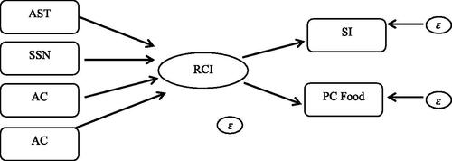
The updated RIMA-II approach defines resilience as a latent construct, the RCI, with multiple predictors and multiple outcomes. The predictors are grouped into four categories (referred to as pillars), namely: (1) Access to basic services (ABS); (2) Ownership of assets (AST); (3) Access to social safety nets (SSN); and (4) Household adaptive capacity (AC). A description of these pillars is shown in Table 2. Each pillar is itself a latent variable determined by a number of observed household level indicators. The household is considered the unit of analysis because it is the unit of decision making for household production and consumption. The outcomes of resilience are per capita food consumption and the Simpson’s dietary diversity index (SI).

Table 2. RIMA resilience pillars

Pillar	Definition
Adaptive capacity (AC)	Adaptive Capacity is the ability of a household to adapt to a new situation and develop new livelihoods strategies.
Social safety nets (SSN)	The Social Safety Nets pillar measures the ability of households to access help from relatives and friends, from government and timely and reliable assistance provided by international agencies, charities, and NGOs.
Assets (AST)	Assets comprise both productive and non-productive assets. Productive assets are the key elements of a livelihood, enabling households to produce consumable or tradable goods. Examples of indicators include land, livestock and durables. Context-specific sets of productive assets which are able to determine the creation of the household income are evaluated. Other tangible nonproductive assets, such as house, vehicle, and household amenities reflect living standards and wealth of a household.
Access to basic services (ABS)	Access to Basic Services shows the ability of a household to meet basic needs, and access and effective use of basic services; for example, access to schools, health facilities; infrastructures and markets.

Source: FAO (2016).

Empirically, the RCI is estimated using the Multiple Indicator and Multiple Outcome model (MIMIC) in a structural equation framework. The conceptual path diagram for the model is depicted in Figure 1. Each pillar is separately estimated using factor analysis of the variables that make up the dimension. The predicted value of each of the components is standardized to range from 0 to 100 and in-turn used to construct the RCI in the MIMIC model. In the MIMIC estimation that we conduct below, several approaches are used to estimate the weights as check for robustness and to eliminate any bias on the weights due to the treatment. The weights represent the relative importance of each pillar to the RCI. In theory, there are four different samples that can be used to generate the weights: (1) only C households at baseline and endline; (2) baseline T and C households; (3) baseline T and C and endline C households; (4) using all the data. Similar to D’Errico et al. (2020), we find that the results are consistent across the various specifications and we proceed with the model that makes use of all the data since this is the most efficient (FAO, 2016).

Figure 1. The MIMIC conceptual framework.

Given that the data used for the analysis was not designed to explicitly apply the RIMA model, a few adaptations were necessary before estimating the RCI. Table 3 shows the indicators proposed by the FAO for each pillar and the corresponding indicators that we have available from the SCTP instrument. The outcome variables of per capita food expenditure and the Simpson’s index are identical to those proposed under RIMA, as are the AST indicators of asset ownership (agricultural and non-agricultural) and livestock. For SSN, we have total in-kind transfers, whether or not the household is credit constrained and self-reported perceived available support in times of need. Credit constraints and perceived available support capture a potential for support when shocks set in, and thus are very appropriate for capturing resilience. We recognize a potential downside to using the variable of in-kind assistance as a measure of resilience. Households that are better off by themselves may have little in-kind assistance, especially in ‘normal’ times, and so the indicator of whether support can be activated when needed is likely a more appropriate ex-ante measure.

Table 3. RIMA domain indicators by FAO and SCTP equivalents

Domain	FAO suggested indicators	SCTP equivalents/proxies
Outcome indicators	Average per person daily income, Average per person daily expenditure, Food consumption score/other nutrition proxy, dietary diversity and food frequency score, dietary energy consumption	V1. Per capita food expenditure V2. Simpson’s Diversity Index
AST	Agricultural assets, non-agricultural assets, tropical livestock units (TLU), land owned	V3. ‘Wealth’ index of agric assets, durable goods, housing and household characteristics V4. Per capita TLU owned V5. Per capita total land cultivated
SSN	Amount of cash and in-kind assistance, social networks, frequency of assistance, formal/informal transfers	V6. Log of total in-kind transfers V7. Log of value of free maize V8. Credit constraint V9. Perceived available support in times of need
AC	Diversity of income sources, educational level (household average), employment ratio, available coping strategies	V10. Number of income sources V11. Labor constraint V12. Not crop production only household
ABS	Access to schools, hospitals, markets, paved roads, water, waste disposal facilities	Not available

On AC, we have an indicator on number of income sources (income diversity) and the ratio of fit-to-work (FTW) to non-fit-to-work (NFTW) to capture potential labor supply and the dependency ratio. Ideally, we would prefer to have the total income from each of these domains as a more direct measure of capacity and importance to household livelihood, but these were not collected in the survey instrument. We also have a binary variable of whether the household only engages in agriculture or if it combines agriculture with other income generating activities. While education is conceptually a part of AC, in our population there is hardly any variation in schooling of the recipient, over 90 per cent are not literate. ABS indicators consider the availability and quality of infrastructure and amenities—access to schools, hospitals and other health facilities, paved roads, markets, safe houses, water, and waste disposal systems. For the pillar of ABS, we do not have any direct measures to construct an index. While this will affect an individual household’s RCI level and the validity tests, it should not affect our estimates of program impact due to the randomization of households to study arm, provided that randomization worked (which we assess in the next section). Each measured variable is constructed to be positive such that more is better, and for binary variables, the better outcome is coded as one.

4. Data, balance, attrition, and descriptive statistics

4.1. Assessment of randomization

To assess the success of the randomization, we check for baseline balance between T and C households on several indicators. We present results of the balance tests on selected variables in Tables 4–6. Table 4 shows the balance test for characteristics of the household head including sex, age, marital status, education and disability status. Table 5 shows the balance tests for household demographic characteristics, such as the age composition, household size, presence of orphans and disabled members, and dependency structure. Table 6 shows the balance test for the analytic variables used for the resilience modelling (as outlined in Table 3). The tables show the means for T and C, the mean difference, and a t-test of equality of the means. We find that T and C are balanced on all these indicators which gives assurance of successful randomization. Tests of balance for many more variables are provide in the publicly available evaluation reports and all evidence indicates that the randomization was successful at achieving the ideal counterfactual to estimate treatment effects.

Table 4. Test of balance in head characteristics between T and C households at BL

	Control		Treatment		Mean	Diff
HH head characteristics	Mean	N1	Mean	N2	Diff	SE	p-Value
Female	0.83	1,853	0.82	1,678	−0.01	0.02	0.53
Age (years)	56.99	1,853	59.27	1,678	2.28	2.30	0.33
Widow	0.42	1,853	0.45	1,678	0.03	0.04	0.50
Divorced/separated	0.26	1,853	0.23	1,678	−0.03	0.03	0.19
Ever attended school	0.30	1,853	0.29	1,678	−0.01	0.05	0.93
Has chronic condition	0.42	1,853	0.48	1,678	0.06	0.05	0.16
Has a disability	0.11	1,853	0.12	1,678	0.01	0.02	0.75

Table 5. Test of balance in household demographics between T and C households at BL

	Control		Treatment		Mean	Diff
Demographic characteristics	Mean	N1	Mean	N2	Diff	SE	p-Value
Household size	4.45	1,853	4.39	1,678	−0.06	0.24	0.81
Children 0–4 years	0.55	1,853	0.53	1,678	−0.02	0.06	0.76
Children 5–17 years	2.19	1,853	2.10	1,678	−0.08	0.14	0.55
Adults aged 18–64 years	1.10	1,853	1.07	1,678	−0.03	0.11	0.76
Elderly (65+)	0.60	1,853	0.68	1,678	0.08	0.06	0.17
Orphaned	0.91	1,853	0.98	1,678	0.07	0.12	0.56
Disabled	0.19	1,853	0.20	1,678	0.00	0.02	0.86
Of working age (15–64)	1.44	1,853	1.40	1,678	−0.03	0.13	0.80
Dependent (<15 or >64 years)	3.01	1,853	2.99	1,678	−0.02	0.14	0.86
Currently attending school	1.63	1,853	1.55	1,678	−0.08	0.14	0.57

Table 6. Test of balance in resilience estimation indicators between T and C households at BL

	Control		Treatment		Mean	Diff
RIMA input indicators	Mean	N1	Mean	N2	Diff	SE	p-Value
PC food expenditure (MWK)	34,738.50	1,853	37,897.30	1,675	3,158.80	3,102.49	0.32
Simpson's index of dietary diversity	0.59	1,853	0.59	1,657	0.00	0.02	0.83
Asset index	−0.16	1,853	−0.15	1,678	0.02	0.11	0.87
PC TLU	0.01	1,853	0.01	1,678	0.00	0.00	0.82
PC land holding (hectares)	0.46	1,853	0.44	1,678	−0.02	0.09	0.83
Log of in-kind transfer PC	5.40	1,853	5.30	1,678	−0.09	0.50	0.85
Log of value of free maize	0.50	1,853	0.54	1,678	0.03	0.33	0.92
Household credit constrained	0.13	1,853	0.12	1,678	−0.01	0.02	0.80
Perceived available support	1.34	1,853	1.22	1,678	−0.13	0.11	0.25
Income diversification	1.41	1,853	1.44	1,678	0.02	0.05	0.66
HH labor constrain	1.66	1,853	1.59	1,678	−0.07	0.07	0.29
Not crop production only household	0.47	1,853	0.50	1,678	0.03	0.03	0.36

4.2. Attrition

Attrition, when households from the baseline sample are missing in the follow-up surveys, occurs for various reasons, such as migration, death, separation, or the dissolution of households. Overall attrition, when the panel sample differs from the original sample, affects the representativeness of the evaluation results for the population of interest (the SCTP eligible) but remain internally valid. Differential attrition occurs when the treatment and control samples differ in the types of households or individuals who leave the sample, thus eliminating the balance between the T and C groups and leading to biased impact estimates. Ideally, both types of attrition should be null or small.

We investigated attrition at endline for the sample in two ways. First, to test for differential attrition, we checked for similarities at baseline between treatment and control groups for all households that remained in the panel of households, that is, for the households interviewed at baseline and in both follow-up surveys. We tested for overall attrition by comparing the characteristics of households in the panel and the households who were missing at the endline survey. We do not find evidence of differential attrition, meaning that we preserve the balance between the T and C groups found in the baseline survey. However, there is evidence of overall attrition as panel households differ from the lost households in about 8 per cent of the 125 indicators tested for balance in the program report. This is corrected by using inverse probability weighting to adjust the baseline sampling weights. Details of this procedure are available from the authors and are also presented in the publicly available online evaluation reports.

The attrition rates are shown in Table 7 for the overall T and C groups, and also by district. Overall attrition was 6.5 per cent (6% in T and 6.8% in C). The attrition rate was higher in the Mangochi district than in the Salima district (7.1 vs. 5.8%), with the lowest attrition in the T group in Salima (4.9%). Summary attrition tables are given in Appendix Tables A1–A6 for the same variables presented in the balance test in Tables 4–6.

Table 7. Household ‘in the panel’ and attrition rates by T-C status and district

		In panel rate (%)	Attrition rate (%)	N	p-Value (T-C)
Total sample		93.5	6.5	3,531
Treatment group		94.0	6.0	1,678
Control group		93.2	6.8	1,853	0.31
District	Status
Salima	Treatment	95.1	4.9	800
Salima	Control	93.4	6.6	975	0.13
Mangochi	Treatment	92.9	7.1	878
Mangochi	Control	92.8	7.2	878	0.93

5. Empirical results

5.1. MIMIC results and the RCI

Table 8 provides the results of the factor analysis used in constructing the three resilience pillars of AST, SSN and AC. The analysis uses the panel data for both C and T households. The first two factors for each pillar are reported, along with the uniqueness of each variable. However, only the first factor in each case had an eigenvalue greater than one (1). Furthermore, the first factor explains more than 70 per cent of the variance in each pillar (72% for AST, 76% for SSN, and 74% for AC). Estimation of each pillar therefore uses only the first factor loadings.

Table 8. Factor loading and uniqueness for individual indicators by pillar

Variable	Factor1	Factor2	Uniqueness
	Assets (AST) pillar
PC TLU	0.2843	0.1883	0.8837
PC land holding (Acres)	0.3040	−0.1821	0.8744
Wealth index	0.4606	0.0039	0.7878
	Social safety net (SSN) pillar
Perceived support	0.2565	0.1919	0.8912
Value of social network	0.5410	0.0352	0.7059
Log of free maize	0.4245	−0.1956	0.7814
Credit constraint	0.0837	0.1767	0.9530
	Adaptive capacity (AC) pillar
Non-agri household	0.2910	−0.1740	0.8851
Income diversification	0.4294	0.0099	0.8155
Labour Constraint	0.2456	0.1888	0.9040

The coefficients indicate the strength of the relationship between the variables and the latent pillar. For AST, the wealth index shows the greatest strength while value of social network shows the greatest association with the SSN pillar and livelihood diversification shows the greatest association with the AC pillar. The uniqueness describes the proportion of the variance that is unique to the variable and not shared with other variables. Uniqueness typically is inversely related to the factor loadings such that variables with higher uniqueness have lower association with the latent factor. Looking at the uniqueness column, we find that each variable has uniqueness of more than 70 per cent, which can be interpreted to mean that there is no single variable with high dominance in explaining the variance structure for each pillar.

Using the results in Table 8 we generate the synthetic index for each pillar based on the first factor loading and estimate the MIMIC—we show these results in Figure 2. All coefficients are statistically significant at 1 per cent level. The coefficient of per capita consumption is standardized to one to make the coefficient of the Simpson’s index interpretable. We find that a unit increase in the RCI results in a 0.13 increase in the standard deviation of the Simpson’s index. The summary model fit statistics indicate that the chi-square value is significant at the 1 per cent level (Table 9), and the root mean square estimate (RMSEA) is 0.0947 with a p-value of 0. The comparative fit index (CFI) is 0.93 which is >0.9, a threshold widely considered as being indicative of a good model fit. The Tuker-Lewis index (TLI) is also quite high at 0.76 although it falls below the threshold of 0.95 considered as threshold for a good fit. Taken together, having highly significant chi-square and RMSEA values, along with above threshold CFI and high value of TLI suggests a good model fit, an important result because as we mentioned earlier, the questionnaire was not explicitly designed to measure resilience but rather was a multi-topic household survey modelled after the Malawi Integrated Household Survey. This suggests that similar living conditions type surveys that are quite common in sub-Saharan Africa could be used to obtain reasonable estimates of resilience using the RIMA approach.

Figure 2. Schematic representation of RIMA II MIMIC model and results.

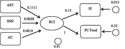
Table 9. Summary model fit statistics

N	Chi-square (p-val)	RMSEA (p RMSEA < 0.05)	CFI	TLI	CD
6,595	120.3428 (0.0000)	0.0947 (0.0000)	0.9301	0.7554	0.3607

5.2. Predictive validity of the RCI

Before estimating the impact of the SCTP on resilience, we assess the predictive validity of the RCI. An important feature of more resilient households is their ability to withstand and recover from shocks, which in part entails utilizing positive coping strategies, that is, strategies that do not permanently lead to a poverty trap or weaken future resiliency. Since coping mechanisms themselves are not used to build the RCI, they present a straightforward opportunity to assess the performance of the RCI in terms of its ability to predict positive shock response behaviour. More resilient households are expected to be more likely to use positive shock response strategies relative to less resilient households. For this analysis, we restrict the sample to the panel of C households only in order to eliminate the potential confounding effect of the cash transfer (the cash transfer itself will directly affect coping strategies). For an unambiguous intertemporal ordering, we relate the baseline RCI to the endline shock response.

In our data, we ask households whether they had experienced any one of 15 different shocks that affected their household negatively, and their most important coping strategy. Table 10 lists the shocks that households were asked about, with an option to specify any shock not pre-listed. The shocks can be classified as covariate shocks, which affect the entire community or village (such as floods, drought, crop-destroying insects, etc.) or idiosyncratic shocks which are limited to the households (such as death of a breadwinner, catastrophic health expenditure, destruction of dwelling, theft of household goods, etc.). At baseline, about 94 per cent of households reported experiencing at least one of these shocks, and the typical household experienced about three of the shocks. At the endline, about 87 per cent of households reported experiencing at least one of the shocks in the prior 12 months with the typical household experience about two of the shocks. These figures show that these shocks constitute a regular feature of the daily lives of the households, and that resilience is a highly relevant concept in this population. Participation in the SCTP did reduce the share of households reporting at least one shock which suggests that the SCTP had some protective effect on the experience of shocks, or at least on the households’ interpretation of events that are shocks. The covariate shocks were more common than the idiosyncratic shocks (Table A7).

Table 10. List of shocks experienced by households

1	Drought/irregular rains
2	Floods/landslides
3	Unusually high level of crop/livestock pests or disease
4	Unusually low prices for agricultural output
5	Unusually high costs of agricultural inputs
6	Unusually high prices for food
7	End of regular assistance/aid remittances from outside household
8	Serious illness or accident of household member(s)
9	Birth in the household
10	Death of household income earner(s)
11	Break-up of household (divorce/separation/death/migration)
12	Theft of money/valuables/assets/agricultural output
13	High education costs
14	House destroyed (for example, burning, flood, winds)
15	Other(s)

Coping with these shocks usually includes a mix of strategies, some negative (such as reducing consumption or sending children out to work), some positive (relying on own savings/SCTP payment, receiving unconditional help from social networks), and some ambiguous depending on the extent of the response relative to the initial conditions (e.g. labor intensification could be positive or negative depending on the initial level of labor supply). Table 11 shows the schema used for the classification of coping mechanisms as positive, negative or ambiguous. Our classification is based on the literature on how credit-constrained rural households in Africa typically self-insure against risk (see the review by Mogues, 2011). The key idea is that credit-constrained households will engage in precautionary savings, typically holding cash or productive assets that are highly liquid and can be exchanged with little or no transaction costs. Small livestock of the type predominant among our study households would fall under this category, as well as grain stores; entering into liquid debt on the other hand is widely considered a negative response by households. For each household, we count the total number of different coping strategies used and then compute the shares for positive, negative and ambiguous strategies, and we also measure liquid debt directly.

Table 11. Classification of coping strategies to shocks

Type of coping strategy	Pos	Neg	Amb
Relied on own savings	‎√
Received unconditional help form relatives/friends	√
Received unconditional help from government	√
Received unconditional help from NGO/Religious institutions	√
Changed eating patterns (relied on less preferred food, reduced portion or number of meals per day, household members skipped days of eating)		√
Employed household members took on more employment			√
Adult HH members who were previously not working had to find work			√
Household members migrated			√
Reduced expenditures on health and/or education		√
Obtained credit/took loan			√
Sold agricultural assets		√
Sold durable assets		√
Sold land/building		√
Sold crop stock	√
Sold livestock	√
Intensified fishing/farming			√
Sent children to live elsewhere		√
Engaged in spiritual efforts			√
Did not do anything		√
SCT Payment	√
Planted trees or built conservation structures	√
Children sent out to work (Ganyu)		√

At baseline, the proportion of coping strategies that were positive was 0.4. In Table 12, we group households into quintiles according to the baseline RCI and report the average proportion of positive coping strategies in each quintile. The results show a high degree of agreement between the RCI and the share of positive responses to shocks that are adopted by households two years in the future and contemporaneously. Looking among the C households, we find that among the least resilient households (those in the bottom quintile of the RCI) at baseline, the average proportion of positive coping to shocks at the endline is 25 per cent compared to 62 per cent among households in the highest RCI quintile at baseline. The relationship is monotonic increasing with higher proportions of positive coping to shocks as households go from the lowest to highest quintile. This pattern is identical when we look at baseline (i.e. contemporaneous) shock responses.

Table 12. Share of positive coping responses to shocks by baseline resiliency quintiles

	Baseline			Endline
Baseline resilience quintile	C	T	Total	C	T	Total
Lowest	0.23	0.29	0.26	0.25	0.63	0.37
Second	0.31	0.34	0.33	0.34	0.67	0.47
Middle	0.42	0.42	0.42	0.40	0.69	0.54
Fourth	0.49	0.47	0.48	0.51	0.76	0.64
Highest	0.59	0.59	0.59	0.62	0.77	0.71
Total	0.39	0.41	0.40	0.40	0.72	0.55

Household quintile rank is based on their baseline resiliency value. The numbers in the table show the proportion of positive coping strategies adopted by the household at baseline and then at endline.

Table 12 also shows results for the treatment group, and we see the same pattern of results, whereby the share of positive coping strategies adopted by households increases as we move from the lowest quintile (least resilient) to the highest quintile. Also of interest in this table is a comparison of the proportions of positive shock responses per household between T and C at baseline and endline. While the proportions are near identical for each quintile at baseline, the proportions of positive coping to shocks are significantly higher at each quintile among T households at endline. As we show in the next section, this is because the actual RCI is higher among T households at endline.

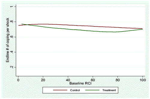
While Table 12 indicates that the relationship between endline coping and the baseline RCI is monotonic, we examine this proposition more closely using a local linear regression relating the RCI score to positive coping—the resulting graph is depicted in Figure 3. This shows that between RCI scores of 20 and 80 (which represents 84% of the sample), the relationship is quite linear, with each unit change in the RCI generating a similar constant increase in the probability of engaging in positive coping mechanisms two years in the future. Figure 4 looks at the number of coping responses adopted by households per shock, though our data is limited to two responses per shock. Here there appears to be little association except for a slight decline in the number of coping per shock among households with high RCI (just 0.10 change in the number of coping mechanisms from the lowest to the highest RCI). What is interesting is that those in the treatment group tend to report fewer number of coping strategies relative to the control group after a threshold of 20 on the resilience scale, suggesting that the cash transfer has allowed households to reduce the number of coping activities required per a given shock.

Figure 3. Future positive coping and baseline RCI among control households.

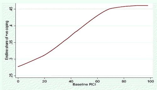
Figure 4. Future number of total coping mechanisms and baseline RCI among control and treatment households.

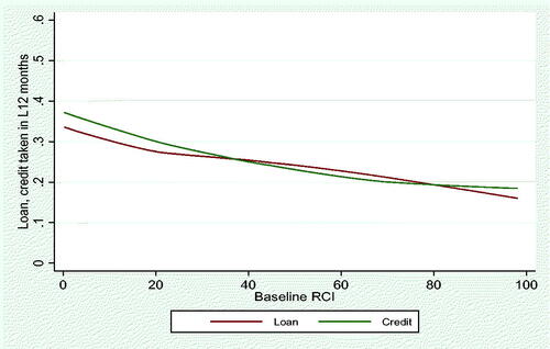
We also look at the correlation between the negative coping strategy of incurring more liquid debt and the baseline resilience scale. Figure 5 shows a very strong negative correlation between baseline resilience and future indebtedness, either measured by cash loans or purchases on credit, again suggesting that the resilience index using the RIMA approach has predictive ability.

Figure 5. Future loan and credit purchases and baseline RCI among control households.

Food security is the ultimate outcome in the RIMA approach, and indeed in almost all studies that examine resilience, so another obvious test of the validity of the RCI is to gauge its predictive ability with respect to future food security. As before, we show four food security indicators at endline by baseline RCI quintile among C households in Table 13. Food consumption and the Simpson’s Index were used to create the RCI, and we also report two other food security indicators—the proportion of households who were worried about food in the last seven days, and the food consumption score (FCS), which is a weighted measure of dietary diversity and nutritional importance of each category. For example, if one household consume food from only two broad categories (tubers and spices) and another household consumes food from only two broad categories (tubers and meat) then the two households would have the same dietary diversity score but different FCS because spices and meat have different weights. For each of the (future) food security indicators we again see a clear increasing monotonic relationship with the baseline quintile ranking on the RCI. These results further suggest that the RCI has predictive validity as a measure of resilience.

Table 13. Baseline resilience and endline food security among C households

Baseline RCI quintiles among C households	Endline food security indicators
	Mean PC food (MWK)	No food worry	Simpson's index	Food consumption score
Lowest	19,790.400	0.053	0.526	6.281
Second	25,427.950	0.057	0.582	7.934
Middle	34,004.360	0.071	0.595	8.873
Fourth	39,047.250	0.140	0.620	9.342
Highest	54,268.380	0.205	0.668	9.703

5.3. Impact of the SCTP on resilience building

We now turn to the main objective of the paper, which is to estimate the impact of the SCTP on resilience. We begin by showing the distribution of the actual RCI scores by treatment status and baseline RCI quintile in Table 14. At baseline, given the randomized design of the study, we expect the scores to be balanced across the study arms and this is what we find in the first two columns of Table 14. We conducted t-tests for mean differences in the baseline RCI score across the two groups and found no statistically significant differences in the RCI score at BL but a statistically significant difference at endline.

Table 14. RCI score by treatment status and wave

	Baseline			Endline
Resilience quintiles	C	T	All	C	T	All
Lowest	19.0	19.2	19.1	18.0	21.8	18.5
Second	33.9	34.0	34.0	34.0	35.0	34.4
Middle	45.0	44.9	45.0	44.9	45.5	45.2
Fourth	56.3	56.3	56.3	56.9	57.3	57.1
Highest	73.9	75.1	74.5	76.2	76.3	76.2
All	40.7	41.2	40.9	44.9	58.6	51.4

Note: Quintiles are created for the full sample at BL and EL. The overall means are weighted by the share of T and C households in each quintile (Table A8), and this explains why there is an apparent equal distribution of means by quintile, but the overall means are different.

We provide a more formal test of the impact of the SCTP on the RCI using a difference-in-difference (DID) model as follows: $${\mathit{RCI}}_{\mathit{ijt}}={\beta }_0+{\beta }_1{P}_j+{\beta }_2{T}_t+{\beta }_3{P}_j·T_t+{\beta }_4{\mathit{X}}_{ij}+{\epsilon }_{\mathit{ijt}}$$

In this framework, RCI_ijt is the outcome of interest for household i who lives in VC j at time t. $P_j$ is a binary variable set to 1 if VC $j$ is receiving the SCTP programme, and to 0 if it is not. T_t is a dummy (binary) variable for time of the observation, set to 1 if the observation is from the endline survey, and to 0 if it is from the baseline. $P_j·T_t$ is the interaction term of the programme variable and the time dummy, X_ijt represents a set of observed household characteristics, such as household size, household demographic composition, and household head characteristics, all measured at baseline, and, ε_ijt is the usual error term. In this model, the coefficient of main interest is β₃, the coefficient of the interaction term, which is the DID programme impact at endline. Its estimated value (${\widehat{\beta }}_3$) is interpreted as the additional change in the RCI value achieved between baseline and endline as a result of the households receiving the SCTP, relative to the change occurring in the comparison group, controlling for differences in the baseline values of the observed characteristics, X_ijt.

We use cluster-robust standard errors to account for the lack of independence across observations due to clustering of households within VCs. We also use inverse probability weighting to adjust the sampling weights to account for the six per cent attrition in the follow-up sample. We present the impact for the full sample, for baseline bottom 50 per cent of households by expenditure (for whom the per capita transfer will be much large), baseline small households (household size <5), and baseline labour constrained households (for whom labor shortage might affect resilience capacity).

Estimation results of the DID model are shown in Table 15 along with baseline and endline means for the two study groups for ease of interpreting effect sizes. We see that the SCTP has a statistically significant impact on the RCI score on all the samples shown in the table. For the full sample, the point estimate of 12.43 percentage points implies an effect size that is 30 per cent of the baseline mean value. For baseline poorest households, the effect size is almost double that at 51 per cent of the baseline mean score. A kernel density of the RCI by treatment status over time is shown in Figure 6. We find a clear increase in the distribution of the resilience scores for the T group at endline compared to the near identical resilience distribution of C and T at baseline.

Figure 6. RCI by treatment status and time.

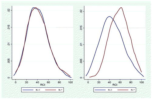
Table 15. Impacts on resilience capacity index (overall and heterogeneous)

Dependent	Endline	Baseline	Baseline	Endline	Endline
Variable	Impact	Treatment mean	Control mean	Treated mean	Control mean
	(1)	(2)	(3)	(4)	(5)
Full sample	12.432***	42.144	41.493	58.457	45.076
	(7.67)
N	6,472	1,556	1,686	1,532	1,698
Baseline poorest 50%	14.516***	28.249	28.114	54.380	38.462
	(9.87)
N	3,283	780	853	785	865
Baseline small households	11.797***	48.970	48.854	62.482	49.456
	(6.28)
N	3,188	782	826	753	827
Baseline labour constrained households	13.144***	41.806	40.952	58.189	44.073
	(7.88)
N	5,236	1,302	1,369	1,231	1,334

Notes: Estimations use difference-in-differences modelling among panel households. Binary outcomes are estimated using LPM. All estimations control for baseline head of household’s characteristics (age in years, sex, indicator of any schooling, indicator of literacy, marital status), household demographic composition and size, indicators for new household members and household member outmigration, and a vector of contemporaneous cluster level prices. Robust t-statistics were obtained clustering at the different levels of the sampling design and are shown in parenthesis. *** 1 per cent significance.

To unpack the pathway through which the SCTP impacts on the RCI, we examine the program impacts on each of the resilience input variables as well as on the pillars. Table 16 gives the results of the impacts. We see significant positive impacts on the AST pillar as a whole, driven by positive impacts on asset holdings and the TLU. We also find significant positive impact on AC, driven by increased income diversification. However, we do not find impacts on the pillar of SSN and the input variables. We estimated Lee Bounds (without covariates) for the treatment effect on RCI and its three components. For the three statistically significant effects (RCI, AST and AC), the Lee Bounds do not cross zero. The bound for RCI is 13.22–14.26, the bound for AST is 7.12–8.52 and the bound for AC is 5.32–6.90.

Table 16. Summary impacts on resilience pillars and input variables

Dependent	Endline	Baseline	Baseline	Endline	Endline
Variable	Impact	Treatment mean	Control mean	Treated mean	Control mean
	(1)	(2)	(3)	(4)	(5)
AST	6.893***	29.983	29.890	46.660	38.904
	(6.54)
Asset Index	0.292***	−0.133	−0.162	0.269	−0.228
	(2.84)
PC TLU	0.013***	0.010	0.010	0.027	0.012
	(3.22)
PC Land holding (hectares)	0.018	0.452	0.382	0.414	0.363
	(0.28)
SSN	−2.257	42.247	44.268	37.003	35.964
	(−0.52)
Log of in-kind transfer PC	−0.177	5.378	5.418	4.878	4.495
	(−0.32)
Log of value of free maize	−0.477	0.535	0.502	0.038	0.165
	(−1.51)
Household credit constrained	−0.019	0.124	0.131	0.101	0.109
	(−0.66)
Perceived available support	0.122	1.205	1.335	1.209	1.162
	(0.78)
AC	4.867***	33.001	31.876	46.679	39.527
	(2.93)
Income diversification	0.254***	1.455	1.426	1.799	1.403
	(4.75)
HH labor constrained	0.007	1.593	1.673	1.691	1.729
	(0.14)
Not crop production only household	0.172***	0.499	0.473	0.679	0.438
	(4.75)
N	6,604	1,576	1,726	1,576	1,726

Notes: Estimations use difference-in-differences modelling among panel households. Binary outcomes are estimated using LPM. See Table 15 for additional details of the estimation approach. ***1 per cent significance. Bold values correspond to those for each aggregate pillar.

5.4. Resilience vs. consumption vs. assets

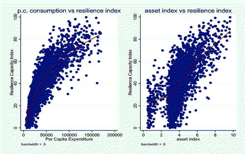
An obvious competing hypothesis would be that baseline consumption or assets could be an equally good predictor of future coping to shocks. Richer households at baseline can be expected to have better coping to shocks in the future in much the same was as better resilience at baseline does. We examine this hypothesis by comparing the strength of the predictive power of resilience to that of consumption. As shown in Figure 7, the association between baseline RCI and endline coping mechanisms to shock is monotonic increasing, while the relationship between baseline consumption and endline positive adaption to shocks is highly non-linear and actually decreases at higher levels of baseline consumption. At baseline the correlation between RCI and per capita consumption was 0.80, and this declined to 0.67 at the endline. The left panel of Figure 8 shows that in fact the relationship is highly non-linear, with substantial variability around the predicted line, indicating that these two measures, while clearly correlated (as theory would suggest they ought to be), are not perfect substitutes for each other. The right panel of Figure 8 shows the relationship between the asset index used in the RIMA model and the RCI. Again, we see that the relationship is highly non-linear, especially at lower levels of the asset index, with considerable variability of RCI at all levels of the asset index.

Figure 7. Endline positive coping to shocks by baseline RCI and baseline consumption.

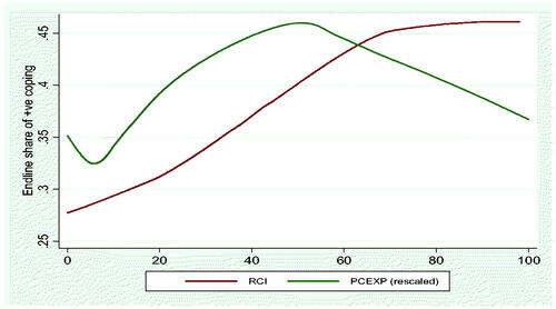
Figure 8. Per capita consumption and asset index vs. RCI—baseline only.

6. Discussion and conclusion

This paper has examined the impacts of Malawi’s SCTP program on development resilience. We find that the SCTP has positively impacted household production, asset ownership, income diversification and strengthening. The SCTP has also improved protective indicators, such as per capita food consumption, dietary diversity and food security. We use the FAO RIMA II model to build an index of development resilience from the data and examine the predictive validity of this index. Increases in the index value are predictive of future positive coping behaviours in the face of shocks and are also predictive of future food consumption and food security. We also compare the predictive power of baseline resilience and baseline consumption and asset holding to future positive coping responses to shocks, and find that resilience is a more consistent predictor of future positive coping to shocks than consumption or assets. Moreover, resilience and consumption are not perfectly correlated, the relationship is highly non-linear suggesting that the two contain different information. These validation results suggest that the RIMA II approach can be used to measure development resilience, for example for profiling and ranking tool for interventions, as well as early warning.

We then estimate the impact of the SCT on household resilience and find that although the SCTP was not explicitly designed with increasing resilience in mind, nonetheless, the SCTP has positively impacted resilience. This is an important result because it suggests that a large-scale government unconditional cash transfer, whose primary objective is short-term protection, can also strengthen household resiliency and thus the ability for ultra-poor households to withstand shocks. Our results are consistent with the one previous study examining the impact of a cash transfer program on resilience using the RIMA approach (D’Errico et al., 2020), who also find that the Lesotho Child Grant Program increases the RCI. However, unlike in Malawi, they do not find strong effects of the cash transfer on the individual components (pillars) of the RCI, while we find strong impacts on assets and adaptive capacity.

A key strength of our study is that it uses a well-designed RCT to estimate the impact of the SCTP on resilience. A weakness of the study is that we do not have the full range of indicators recommended by the RIMA approach. A further limitation is the external validity of the findings, though the Malawi SCTP has similar design parameters to other government cash transfer programs in Africa, which increases the potential for external validity. In terms of future research, with just two studies to date reporting on the resilience effects of national cash transfer programs, more evidence using the RIMA approach is necessary in this area to understand whether cash transfer programs in different contexts can deliver these results, and which specific components of the resilience index are driving the effects on household resilience.

Disclosure statement

No potential conflict of interest was reported by the author(s).

Additional information

Funding

The evaluation of the Malawi Social Cash Transfer Programme was funded by a consortium of donors including the European Union, UNICEF-Malawi, KfW, and 3IE. The evaluation was implemented by the University of North Carolina at Chapel Hill and the Center for Social Research under contract to UNICEF-Malawi. The evaluation would not have been possible without the dedicated work of a large team of collaborators, including technical staff of the implementing Ministry, Ayala Consulting, the Center for Social Research at the University of Malawi, and representatives from the key development partners in Malawi—they are recognized as part of the Evaluation Team. We dedicate this paper to the memory of Harry Mwamlima, a longstanding champion of social protection in the Ministry of Finance, Economic Planning and Development of the Government of Malawi.

Appendix

Table A1. Tests for differential attrition on head characteristics

	Control		Treatment		Mean	Diff
HH Head Characteristics	Mean	N1	Mean	N2	Diff	SE	p-value
Female	0.85	1726	0.82	1577	–0.02	0.02	0.34
Age (years)	56.95	1726	59.01	1577	2.06	2.24	0.37
Widow	0.42	1726	0.44	1577	0.02	0.04	0.55
Divorced/Separated	0.26	1726	0.23	1577	–0.03	0.03	0.28
Ever attended school	0.30	1726	0.30	1577	0.00	0.05	0.98
Currently attending school	0.01	1726	0.01	1577	0.00	0.00	0.30
Highest grade attended	1.06	1726	1.08	1577	0.02	0.20	0.92
Has chronic condition	0.41	1726	0.48	1577	0.06	0.04	0.17
Has a disability	0.11	1726	0.11	1577	0.01	0.02	0.77

Note: p-value is for the statistical test of mean differences between T and C households using baseline data Weighted results; standard errors obtained considering multi-stage sampling design.

Table A2. Tests for differential attrition on household demographics

	Control		Treatment		Mean	Diff
Demographic Characteristics	Mean	N1	Mean	N2	Diff	SE	p-value
Household size	4.52	1726	4.46	1577	–0.05	0.23	0.82
Children 0–4 years	0.55	1726	0.54	1577	–0.01	0.06	0.87
Children 5–17 years	2.24	1726	2.15	1577	–0.09	0.14	0.52
Adults aged 18–64 years	1.12	1726	1.09	1577	–0.03	0.11	0.75
Elderly (65+)	0.60	1726	0.68	1577	0.08	0.06	0.18
Orphaned	0.92	1726	1.00	1577	0.07	0.13	0.57
Disabled	0.19	1726	0.19	1577	–0.00	0.03	0.94
Of working age (15–64)	1.47	1726	1.44	1577	–0.03	0.13	0.82
Dependent (<15 or >64 years)	3.05	1726	3.03	1577	–0.03	0.13	0.84
Currently attending school	1.67	1726	1.58	1577	–0.09	0.14	0.51

Note: p-value is for the statistical test of mean differences between T and C households using baseline data Weighted results; standard errors obtained considering multi-stage sampling design.

Table A3. Tests for differential attrition on resilience estimation indicators

	Control		Treatment		Mean	Diff
RIMA input indicators	Mean	N1	Mean	N2	Diff	SE	p-value
PC Food expenditure (MWK)	34,259.12	1726	37,073.50	1574	2,814.38	3,097.94	0.37
Simpson's Index of dietary diversity	0.59	1726	0.59	1577	0.00	0.02	0.83
Asset Index	–0.16	1726	–0.13	1577	0.03	0.10	0.79
PC TLU	0.01	1726	0.01	1577	0.00	0.00	0.84
PC Land holding (hectares)	0.38	1726	0.45	1577	0.07	0.06	0.27
Log of in-kind transfer PC	5.42	1726	5.38	1577	–0.04	0.51	0.94
Log of value of free maize	0.50	1726	0.53	1577	0.03	0.33	0.92
Household credit constrained	0.13	1726	0.12	1577	–0.01	0.02	0.74
Perceived available support	1.34	1726	1.21	1577	–0.13	0.11	0.24
Income diversification	1.43	1726	1.46	1577	0.03	0.05	0.58
HH labor constrain	1.67	1726	1.59	1577	–0.08	0.06	0.22
Not crop production only household	0.47	1726	0.50	1577	0.03	0.03	0.46

Note: p-value is for the statistical test of mean differences between T and C households using baseline data Weighted results; standard errors obtained considering multi-stage sampling design.

Table A4. Tests for selective attrition on head characteristics

	Attriters		Panel HHs		Mean	Diff
HH head characteristics	Mean	N1	Mean	N2	Diff	SE	p-value
Female	0.73	228	0.84	3303	0.10	0.03	0.00
Age (years)	60.02	228	57.97	3303	–2.05	1.96	0.30
Widow	0.48	228	0.43	3303	–0.05	0.04	0.18
Divorced/Separated	0.22	228	0.25	3303	0.03	0.03	0.44
Ever attended school	0.27	228	0.30	3303	0.02	0.04	0.56
Currently attending school	0.01	228	0.01	3303	–0.01	0.01	0.43
Highest grade attended	1.10	228	1.07	3303	–0.02	0.19	0.90
Has chronic condition	0.53	228	0.44	3303	–0.09	0.03	0.01
Has a disability	0.21	228	0.11	3303	–0.11	0.03	0.00

Note: p-value is for the statistical test of mean differences between the panel sample and the attriter sample using baseline data Weighted results; standard errors obtained considering multi-stage sampling design.

Table A5. Tests for differential attrition on household demographics

	Attriters		Panel HHs		Mean	Diff
Demographics characteristics	Mean	N1	Mean	N2	Diff	SE	p-value
Household size	3.47	228	4.49	3,303	1.03	0.18	0.00
Children 0–4 years	0.48	228	0.55	3,303	0.07	0.05	0.20
Children 5–17 years	1.50	228	2.19	3,303	0.69	0.14	0.00
Adults aged 18–64 years	0.82	228	1.11	3,303	0.29	0.05	0.00
Elderly (65+)	0.66	228	0.64	3,303	−0.02	0.04	0.67
Orphaned	0.69	228	0.96	3,303	0.27	0.11	0.02
Disabled	0.26	228	0.19	3,303	−0.07	0.04	0.06
Of working age (15–64)	1.02	228	1.45	3,303	0.44	0.07	0.00
Dependent (<15 or >64 years)	2.45	228	3.04	3,303	0.59	0.13	0.00
Currently attending school	1.13	228	1.63	3,303	0.50	0.14	0.00

Note: p-value is for the statistical test of mean differences between the panel sample and the attriter sample using baseline data Weighted results; standard errors obtained considering multi-stage sampling design.

Table A6. Tests for selective attrition on resilience estimation indicators

	Attriters		Panel HHs		Mean	Diff
RIMA input indicators	Mean	N1	Mean	N2	Diff	SE	p-value
PC Food expenditure (MWK)	44,675.99	228	35,651.42	3300	–9024.57	2695.39	0.00
Simpson's Index		0	0.59	3303	0.00	0.00
Asset Index	–0.25	228	–0.15	3303	0.10	0.10	0.32
PC TLU	0.01	228	0.01	3303	0.00	0.00	0.90
PC Land holding (hectares)	0.95	228	0.42	3303	–0.53	0.57	0.36
Log of in-kind transfer PC	4.74	228	5.40	3303	0.66	0.29	0.03
Log of value of free maize	0.54	228	0.52	3303	–0.02	0.10	0.83
Household credit constrained	0.11	228	0.13	3303	0.02	0.02	0.21
Perceived available support	1.40	228	1.27	3303	–0.13	0.07	0.06
Income diversification	1.23	228	1.44	3303	0.21	0.07	0.01
HH labor constrain	1.47	228	1.63	3303	0.16	0.06	0.01
Not crop production only household	0.42	228	0.49	3303	0.06	0.05	0.20

Note: p-value is for the statistical test of mean differences between the panel sample and the attriter sample using baseline data Weighted results; standard errors obtained considering multi-stage sampling design.

Table A7. Impacts on shocks and coping

Dependent	Endline	Baseline	Baseline	Endline	Endline
variable	impact	treatment Mean	control Mean	treated Mean	control Mean
	(1)	(2)	(3)	(4)	(5)
Experienced any shock with negative effect	–0.059**	0.953	0.933	0.858	0.916
	(–2.28)
Number of different shocks	–0.096	2.516	2.450	2.248	2.363
	(–0.51)
Experienced any covariate shock	–0.076**	0.923	0.902	0.828	0.894
	(–2.19)
Number of covariate shocks	–0.060	2.118	2.049	1.783	1.803
	(–0.42)
Experienced any idiosyncratic shock	–0.006	0.266	0.267	0.138	0.166
	(–0.16)
Number of idiosyncratic shocks	–0.021	0.309	0.303	0.156	0.200
	(–0.47)
Share of positive coping responses	0.244***	0.421	0.397	0.695	0.404
	(3.56)
Share of negative coping responses	–0.224***	0.245	0.188	0.290	0.493
	(–3.71)
N	6119	1508	1634	1383	1594

Note: Estimations use difference-in-differences modelling among panel households. Binary outcomes are estimated using LPM. See Table 15 for additional details of the estimation approach. * 10% significance ** 5% significance; *** 1% significance.

References

- Alfani, F., Dabalen, A., Fisker, P., & Molini, V. (2015). Can we measure resilience? A proposed method and evidence from countries in the Sahel. World Bank Policy Research Working Paper No. 7170.
- Alinovi, L., D’Errico, M., Main, E., & Romano, D. (2010). Livelihoods strategies and households resilience to food security: An empirical analysis to Kenya.
- Ayala Consulting (2012). Malawi social cash transfer inception report. Lilongwe: Ayala Consulting.
- Bahadur, A., Ibrahim, M., & Tanner, T. (2013). Characterising resilience: unpacking the concept for tackling climate change and development. Climate and Development, 5(1), 55–65. doi:10.1080/17565529.2012.762334
- Barrett, C., & Constas, M. A. (2014). Towards a theory of resilience for international development applications.
- Bhalla, G., Handa, S., Angeles, G., & Seidenfeld, D. (2016). The effect of cash transfers and household vulnerability on food insecurity in Zimbabwe.
- Carolina Population Center (2016). Malawi social cash transfer programme endline impact evaluation report. Retrieved from https://transfer.cpc.unc.edu/wp-content/uploads/2021/04/Malawi-SCTP-Endline-Report_Final.pdf
- Catholic Relief Services (2013). Niger resilience study. Baltimore, MA: Catholic Relief Services.
- Cisse, J., & Barrett, C. (2018). Estimating development resilience: A conditional moments-based approach. Journal of Development Economics, 135, 272–284. doi:10.1016/j.jdeveco.2018.04.002
- D’Errico, M., Garbero, A., Letta, M., & Winters, P. (2020). Evaluating program impact on resilience: Evidence from Lesotho’s child grants programme. The Journal of Development Studies, 56(12), 2212–2234.
- DFID 2011. Defining disaster resilience: A DFID approach paper. London. Retrieved from https://www.gov.uk/government/publications/defining-disaster-resilience-a-dfidapproach-paper
- FAO 2016. Resilience index measurement and analysis II. Rome: Food and Agricultural Organization of the United Nations.
- Food Security Information Network-Resilience Measurement Technical Working Group (2014, January). Resilience measurement principles. FSIN Technical Series No. 1.
- Frankenberger, T., Mueller, M., Spangler, T., & Alexander, S. (2013). Community resilience: Conceptual framework and measurement feed the future learning agenda. Rockville, MD: Westat.
- Handa, S., Natali, L., Seidenfeld, D., Tembo, G., & Davis, B. (2018). Can unconditional cash transfers raise long-term living standards? Evidence from Zambia. Journal of Development Economics, 133, 42–65. doi:10.1016/j.jdeveco.2018.01.008
- Handa, S., Otchere, F., & Sirma, P. 2022. More evidence on the impact of government social protection in Sub-Saharan Africa: Ghana, Malawi and Zimbabwe. Development Policy Review, 40(3), 1–22. doi:10.1111/dpr.12576
- Hjelm, L., Mathiassen, A., & Wadhhwa, A. (2016). Food and nutrition policy measuring poverty for food security analysis: Consumption-versus asset-based approaches. Food and Nutrition Bulletin, 37(3), 275–289.
- Kimetrica (2015). Measuring climate resilience and vulnerability: A case study from Ethiopia. In FEWSNet (Ed.), Famine early warning systems network. Washington, DC: United States Agency for International Development.
- Knippenberg, E., Jensen, N., & Constas, M. (2019). Quantifying household resilience with high-frequency data: Temporal dynamics and methodological options. World Development, 121, 1–15.
- Mogues, T. (2011). Shocks and asset dynamics in Ethiopia. Economic Development & Cultural Change, 60(1), 91–120. doi:10.1086/661221
- OXFAM (2013). A multidimensional approach for measuring resilience. OXFAM GB Working Paper. Retrieved from http://policypractice.oxfam.org.uk/publications/a-multidimensional-approach-to-measuring-resilience-302641
- Resilience Alliance 2002. Key concepts. Retrieved from http://www.resalliance.org/index.php/key_concepts
- Signorelli, S., Azzarri, C., & Roberts, C. (2016). Malnutrition and climate patterns in the ASALs of Kenya: A resilience analysis based on a pseudo-panel dataset (Vol. 2). Washington, DC: International Food Policy Research Institute.
- Smith, L. C., & Frankenberger, T. R. (2018). Does resilience capacity reduce the negative impact of shocks on household food security? Evidence from the 2014 floods in Northern Bangladesh. World Development, 102(C), 358–376. doi:10.1016/j.worlddev.2017.07.003
- Walsh, F. (2003). Family resilience: a framework for clinical practice. Family Process, 42(1) 1–18. doi:10.1111/j.1545-5300.2003.00001.x
- Winder Rossi, N., Spano, F., Sabates-Wheeler, R., & Kohnstamm, S. 2017. Social protection and resilience. Supporting livelihoods in protracted crises, fragile and humanitarian context. FAO Position Paper. Rome: Food and Agriculture Organization of the United Nations, Institute for Development Studies.
- Winderl, T. (2014). Disaster resilience measurements: Stocktaking of ongoing efforts in developing systems for measuring resilience. United Nations Development Programme (UNDP). Retrieved from http://www.preventionweb.net/files/37916_disasterresiliencemeasurementsundpt.pdf