Hydraulic resistance in open-channel flows over self-affine rough beds

ABSTRACT

Knowledge of hydraulic resistance of single-valued self-affine fractal surfaces remains very limited. To advance this area, a set of experiments have been conducted in two separate open-channel flumes to investigate the effects of the spectral structure of bed roughness on the drag at the bed. Three self-affine fractal roughness patterns, based on a simple but realistic three-range spectral model, have been investigated with spectral scaling exponents of −1, −5/3 and −3, respectively. The different widths of the flumes and a range of flow depths also afforded an opportunity to consider effects of the flow aspect ratio and relative submergence. The results show that with all else equal the friction factor increases as the spectral exponent decreases. In addition, the relationship between the spectral exponent and effective slope of the roughness is demonstrated, for the first time. Aspect ratio effects on the friction factor within the studied range were found to be negligible.

Keywords:

• Bed roughness
• drag coefficient
• hydraulic resistance
• open-channel flow turbulence
• self-affine fractal surface

1 Introduction

Most natural and industrial flows encounter and are influenced by the effects of bed surface roughness. Despite longstanding efforts, the difficulty remains to identify the key roughness parameters that control hydraulic resistance. A fundamental part of the problem exists around properly quantifying the surface roughness. Grinvald and Nikora (1988) classified the roughness descriptions into two general approaches: (1) a “discrete” approach when the roughness is considered as a combination of discrete roughness elements characterized by a set of linear scales and/or their combinations (e.g. length, height, width, steepness and spacing); and (2) a “continuous” approach when the rough surface is considered as a random field of surface elevations characterized by various-order statistical moments (e.g. standard deviation, skewness and kurtosis) and moment functions (e.g. spectra, correlation functions and structure functions).

The popularity of the discrete approach lies in its simplicity and stems from the early work of Nikuradse (1933), who extensively studied roughness effects of densely-packed uniform sand in pipes. He found that the single parameter (sand diameter) can serve as a sufficient descriptor of such surface roughness. For more complex rough surfaces, that need multiple parameters to be properly described, it was proposed that their hydrodynamic effects can be represented by an “equivalent sand roughness height” that produces the same resistance equations as densely-packed uniform sand (Schlichting, 1979). A drawback of the discrete approach is its inability to describe random surfaces, where unambiguous identification of discrete roughness elements is difficult, if possible at all. The continuous approach, on the other hand, treats any surface topography as a random field of elevations, which can then be completely characterized through its $m$-dimensional probability distribution as $m\to \mathrm{\infty }$ (e.g. Bendat & Piersol, 2010). In reality this is rarely known, but an acceptable alternative is to employ a simplified statistical model of the roughness. For instance, based on the assumption that the surface is homogeneous and Gaussian then the second-order moment functions will yield full information about the bed elevation field. Comparisons of discrete and continuous approaches highlight the second, “continuous”, approach as more robust and suitable for description of complex surfaces (e.g. Flack & Schultz, 2010; Nikora, Goring, & Biggs, 1998), although a combination of both approaches may also be beneficial (e.g. Nikora & Goring, 2004). The study reported in this paper is based on the continuous approach as it is deemed more appropriate for a very wide class of natural and technical surfaces.

Following the continuous approach, Nikora et al. (1998) proposed that hydraulic resistance in gravel-bed rivers could be described as a function of three roughness length scales, $l_x$, $l_y$ and ${\sigma }_z$, assuming the universality of the spectral scaling exponent $\beta$ of the bed roughness. Here $l_x$ and $l_y$ are longitudinal and transverse correlation length scales, respectively, and ${\sigma }_z$ denotes the standard deviation of the bed elevations. However, a further generalization can be made by also incorporating the influence of the spectral slope $\beta$, which is an important parameter for characterizing a class of surfaces known as self-affine fractals (e.g. Turcotte, 1997). Among other properties, a cross-sectional profile through a self-affine surface will have a power spectrum which exhibits a power law dependence on wavenumber, at least over a certain range of scales (e.g. Turcotte, 1997). The magnitude of the power law scaling is related to the Hurst exponent $\alpha$ (named after Hurst, 1951) through the expression $\beta =2\alpha +1$. The Hurst exponent can take a value between 0 and 1, with $\alpha =1$ corresponding to the special case of self-similarity, thus yielding limits for $\beta$ from 1 to 3 for a surface to be classified as self-affine fractal (e.g. Turcotte, 1997). Many natural and man-made surfaces exhibit self-affine fractal properties such as the topography of the ocean floor (Bell, 1975), gravel bed rivers (Nikora et al., 1998; Singh, Porté-Agel, & Foufoula-Georgiou, 2010), sand dune river beds (Hino, 1968; Nikora, Sukhodolov, & Rowinski, 1997), machined surfaces (Majumdar & Tien, 1990) and even the surfaces of other planets such as Mars (Nikora & Goring, 2004). Despite this, the systematic study of bed roughness based on continuous self-affine fractals and their corresponding influence on flow resistance has to date received little attention, if any.

This study seeks to address this issue by investigating the influence of spectral structure of bed surface roughness on the hydraulic resistance. A secondary objective is to investigate the effects of relative submergence and channel aspect ratio. To achieve these aims a set of experiments have been carried out to measure the friction factor in two separate open-channel flumes, the first having a width of 1.18 m and the second a width of 0.40 m.

Following the introduction, Section 2 briefly discusses available flow resistance coefficients and considers the partitioning of the measured total surface shear stress before describing a simple spectral roughness model. Section 3 then outlines the design and manufacturing of three self-affine roughness patterns built following the spectral roughness model. Section 4 provides details of the experimental set-up. The effects of relative submergence, roughness structure and channel aspect ratio on flow resistance are explored in Section 5, while Section 6 closes with conclusions.

2 Conceptual background

2.1 Flow resistance formulae

Three commonly cited expressions linking mean flow velocity to hydraulic resistance are those of Chézy, Manning, and Darcy–Weisbach, and can be summarized as: (1) $U=C(RS{)}^{1/2}=\frac{1}{n}{R}^{2/3}{S}^{1/2}={\left(\frac{8gRS}{f_R}\right)}^{1/2}$(1) where $U$ is the bulk flow velocity (depth-averaged or cross-sectionally averaged); $C$ is the Chézy coefficient; $R=A/P$ is the hydraulic radius, $A$ is the cross-sectional area of the flow, $P$ is the wetted perimeter; $S$ is the water surface slope (equal to the bed slope $S_b$ in uniform flow); $n$ is the Manning coefficient; $g$ is gravity acceleration; and $f_R$ is the Darcy–Weisbach friction factor defined in terms of $R$. This study deals with the Darcy–Weisbach friction factor but due to Eq. (1) the results based on the friction factor are also transferable to $n$ and $C$.

Corresponding formulae for the prediction of the friction factor based on properties of the roughness in open-channel flow may be broadly categorized into two groups. The first type of resistance formulae is logarithmic, of the form: (2) ${\left(\frac{8}{f_R}\right)}^{1/2}=m_1\ln \left(\frac{R}{\mathrm{\Delta }}\right)+c_1$(2) where $m_1$ and $c_1$ are numerical constants and Δ is a characteristic roughness length scale. Keulegan (1938) was the first to derive this kind of relationship for the friction factor in open-channel flow by integrating an assumed logarithmic velocity distribution across the entire flow depth. The applicability of such a procedure becomes questionable in open-channel flows when the mean flow depth $H$ becomes comparable to Δ (e.g. Aberle & Smart, 2003). Despite this, the logarithmic type formulas have been observed to satisfactorily predict hydraulic resistance in a number of open-channel studies (e.g. Bathurst, 1985; Smart, Duncan, & Walsh, 2002). The second type of relationships includes power law type relationships of the general form: (3) ${\left(\frac{8}{f_R}\right)}^{1/2}=c_2{\left(\frac{R}{\mathrm{\Delta }}\right)}^{m_2}$(3) where $c_2$ and $m_2$ are numerical constants. Although seemingly lacking theoretical rigour, such equations have also been found to perform well when treating field data (e.g. Bathurst, 2002; Lee & Ferguson, 2002).

Owing to the largely empirical nature of the resistance formulae quoted in Eqs (2) and (3) there is a high degree of variability in the values of the coefficients between studies such that no general formula yet exists (e.g. Ferguson, 2007). In the present study the suitability of Eqs (2) and (3) to describe the behaviour of the friction factor will be considered in relation to self-affine rough beds. The influence of $\beta$ on the coefficients in Eqs (2) and (3) will also be examined since no such information is currently available.

2.2 Friction factor partitioning

The friction factor is a bulk coefficient and incorporates contributions from the bed and sidewalls. Typical laboratory flume experiments and field studies deal with situations where there is a difference between resistance created by the bed and by the sidewalls/channel banks. In order to improve comparability of the results between studies with a specified bed roughness but varying channel width or sidewall configuration, the influence of the sidewalls on the friction factor values should be removed. Such a procedure is referred to as a sidewall correction and numerous approaches have been proposed (e.g. Einstein, 1942; Knight, Demetriou, & Hamed, 1984; Vanoni & Brooks, 1957). Some comments now follow about the partitioning of the friction factor into its constituent bed and sidewall components. This leads to the definition for upper and lower bounds of the true but unknown bed friction factor.

First, we note that our experiments are aimed at studying steady uniform flow in two separate open-channel flumes, each with a rectangular cross section. Under such conditions the force balance may be written as: (4) $\rho gBHL{S}_b=\int {\int }_{A_{surf}}{\tau }_0(x,y,z)d{A}_{surf}$(4) where $\rho$ is fluid density, $B$ is channel width, $L$ is a section length along the channel, $A_{surf}$ is the total wetted surface area (including both sidewalls and bed), and ${\tau }_0$ is the local shear stress over the wetted bed surface. From Eq. (4) it follows that: (5) ${\overline{\tau }}_0=2\frac{H}{P}{\overline{\tau }}_{0w}+\frac{B}{P}{\overline{\tau }}_{0b}$(5) where $P=B+2H$ is a wetted perimeter for a channel with a rectangular cross section, ${\overline{\tau }}_{0w}$ is the mean sidewall shear stress, ${\overline{\tau }}_{0b}$ is the mean bed shear stress, and the overall mean stress ${\overline{\tau }}_0$ across the whole channel surface is defined from Eq. (4) as: (6) ${\overline{\tau }}_0=\rho gR{S}_b$(6) Noting that the total force acting on the channel surface is $(B+2H){\overline{\tau }}_0=2H{\overline{\tau }}_{0w}+B{\overline{\tau }}_{0b}$ yields another expression involving the bed and wall shear stresses, i.e.: (7) $\rho gH{S}_b=\frac{2H}{B}{\overline{\tau }}_{0w}+{\overline{\tau }}_{0b}$(7) Using Eqs (5) and (7) we can obtain two expressions for the mean bed shear stress: (8) ${\overline{\tau }}_{0b}=\rho gH{S}_b\left(1-\frac{2H}{(2H+B)}\frac{{\overline{\tau }}_{0w}}{{\overline{\tau }}_0}\right)$(8) and (9) ${\overline{\tau }}_{0b}=\rho gR{S}_b\left(1+\frac{2H}{B}\left(1-\frac{{\overline{\tau }}_{0w}}{{\overline{\tau }}_0}\right)\right)$(9) Since the term in parentheses in Eq. (8) must be ≤1 while in Eq. (9) the term in parentheses must be ≥1 the following conditions apply: (10) $\rho gR{S}_b\le {\overline{\tau }}_{0b}\le \rho gH{S}_b$(10) which then shows upper and lower bounds for the actual bed shear stress. Relating Eq. (10) to the friction factors shows that: (11) $f_R\le f_b\le f_H$(11) where $f_R=8gR{S}_b/\rho U^2$, $f_b=8{\overline{\tau }}_{0b}/\rho U^2$, and $f_H=8gH{S}_b/\rho U^2$ are the bulk friction factor, bed friction factor, and depth-based friction factor, respectively. For very wide channels the difference between the friction factors of Eq. (11) is insignificant. In the present study, no attempt is made to apply the sidewall corrections as all known techniques involve certain assumptions, which are difficult to properly test for rough-bed open-channel flows. Instead, the results below are presented in terms of both $f_R$ and $f_H$, noting that the true but unknown bed friction factor $f_b$ lies somewhere between these limits, as illustrated in Eq. (11).

2.3 Spectral model of bed roughness

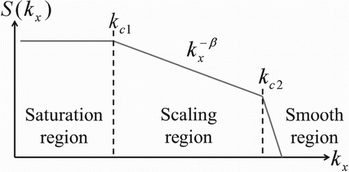
Based on the continuous approach, we can introduce an idealized model of the bed roughness in terms of the wavenumber spectrum, as depicted in Fig. 1. Here, three ranges are distinguishable: (i) a “saturation” (white spectrum) region at low wavenumbers where the roughness amplitudes inversely depend on the roughness lengths; (ii) a scaling region at intermediate wavenumbers where the spectrum decays as a power function with spectral exponent $\beta$; and (iii) a “smooth” region at high wavenumbers where the spectrum rapidly declines to zero (and thus within this region the surface is smooth, i.e. differentiable). The cut-off wavenumbers $k_{c1}$ and $k_{c2}$ define the upper and lower extent of the scaling region, respectively, with $k_{c1}$ providing a measure of the longitudinal and transverse roughness correlation length scales (which also depend on $\beta$), $l_x\sim (k_{xc1}{)}^{-1}$ and $l_y\sim (k_{yc1}{)}^{-1}$ (if considering the model of Fig. 1 in two dimensions, $x$ and $y$). The validity of such a model is supported by measurements of wavenumber spectra in various terrestrial and extra-terrestrial environments (e.g. Hino, 1968; Hubbard, Siegert, & McCarroll, 2000; Nikora & Goring, 2004) and second-order structure functions, which exhibit equivalent distinctive scaling ranges (e.g. Butler, Lane, & Chandler, 2001; Mankoff et al., 2017; Nikora et al., 1998). As it follows from Fig. 1 and assuming a Gaussian random surface, the roughness can be fairly described by the standard deviation of the bed elevations, length scales $l_x$ and $l_y$, a smoothness length scale $l_{sm}\sim (k_{c2}{)}^{-1}$, and the spectral slope $\beta$. If the rough surface is non-Gaussian then additional measures will be required (such as skewness, kurtosis, high-order structure functions, and others). The model of Fig. 1 is used in this study as a foundation for designing three self-affine fractal roughness patterns as described next in Section 3.

Figure 1 Idealized three-range spectral model of bed roughness

3 Self-affine fractal roughness: design and manufacturing

3.1 Numerical design of self-affine rough surfaces

Three self-affine surfaces were designed numerically by the method of spectral synthesis (e.g. Saupe, 1988) to reproduce the roughness model illustrated in Fig. 1. These three self-affine fractal surfaces, referred to hereafter as R1, R2 and R3, were generated using the inverse discrete Fourier transform: (12) $z(x_a,y_b)=\frac{1}{N^2}\sum _{p=0}^{N-1}\sum _{q=0}^{N-1}Z(k_{xp},k_{yq})\exp \left[j2\pi \right(x_a{k}_{xp}+y_b{k}_{yq}\left)\right]$(12) where $z(x_a=a{\mathrm{\Delta }}_x,y_b=b{\mathrm{\Delta }}_y)$ is the roughness height field defined over a periodic domain extending $L_x=N{\mathrm{\Delta }}_x$ and $L_y=N{\mathrm{\Delta }}_y$ in the $x$ and $y$ directions respectively, with $N$ the number of discrete points and ${\mathrm{\Delta }}_x={\mathrm{\Delta }}_y$ the point spacing. The wavenumber vector $(k_{xp},k_{yq})$ is evaluated at the discrete points $k_{xp}=p{\mathrm{\Delta }}_{kx}$ and $k_{yq}=q{\mathrm{\Delta }}_{ky}$ where ${\mathrm{\Delta }}_{kx}=1/N{\mathrm{\Delta }}_x$ and ${\mathrm{\Delta }}_{ky}=1/N{\mathrm{\Delta }}_y$ are wavenumber increments. We use $j=\sqrt{-1}$ to denote the imaginary unit, while $a,b,p$ and $q$ are integers on the interval $[0,N-1]$. The complex valued function $Z(k_{xp},k_{yq})$ was evaluated such that: (1) the two-dimensional power spectral density (Fig. 2a): (13) $S(k_{xp},k_{yq})=\frac{{\mathrm{\Delta }}_x{\mathrm{\Delta }}_y}{N^2}|Z(k_{xp},k_{yq}){|}^2$(13) was radially symmetric, ensuring an isotropic roughness pattern; (2) the phase component $\arg \left[Z\right(k_{xp},k_{yq}\left)\right]$ was uniformly distributed on the interval $[0,2\pi ]$ ensuring a Gaussian probability distribution of the height field $z$; and (3) the one-sided one-dimensional spectrum (Fig. 2b): (14) $S\left(k_{xp}\right)=2\frac{{\mathrm{\Delta }}_x}{N^3}\sum _{q=0}^{N-1}|Z(k_{xp},k_{yq}){|}^{2}p=0,1,2,\dots ,\frac{N}{2}$(14) approximated the model spectrum given by: (15) $S\left(k_x\right)=\left\{\begin{array}{ll}{a}_1& 0<k_x\le k_{c1}\\ a_2{k}_x^{-\beta }& k_{c1}\le k_x\le k_{c2}\\ F\left(k_x\right)& k_x\ge k_{c2}\end{array}\right.$(15) where $a_1$ and $a_2$ are constants, related as $a_2=a_1{k}_{c1}^{\beta }$, and $a_1$ was selected such that the standard deviation of the height field ${\sigma }_z$ was 1.5 mm for all generated roughness patterns. $F\left(k_x\right)$ is a function which decays faster than a power function with exponent −3. The parameters $k_{c1}$ (= 0.02 mm⁻¹) and $k_{c2}$ (= 0.2 mm⁻¹) are the wavenumbers which define the location and extent of the scaling range. The exponent $\beta$ in the scaling range is selected to be 1, 5/3, and 3 for the R1, R2 and R3 roughness designs, respectively. The model spectrum adopted here differs from those in studies of Anderson and Meneveau (2011) and in Barros, Schultz, and Flack (2015), who chose to investigate fractal surfaces having only a single scaling range with no saturation range. Our modelled spectra more closely resemble spectra of real rough surfaces, as highlighted by examples in Section 2.3.

Figure 2 (a) One-dimensional transect through the first quadrant of the two-dimensional power spectrum for the R1, R2 and R3 designs, respectively, as a function of radial wavenumber $k_r$. (b) One-dimensional spectra integrated out of the two-dimensional spectra

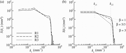
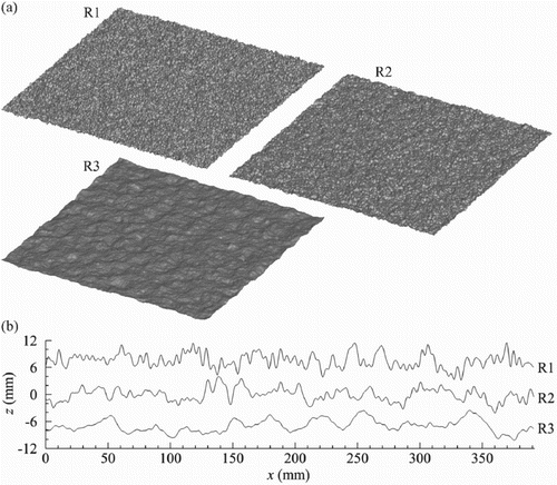
The final three roughness patterns are visualized in Fig. 3a. These numerical patterns have dimensions of 392 mm × 392 mm and are discretized on a 2048 × 2048 point grid. Each surface is isotropic, having identical longitudinal and transverse length scales $l_x=l_y=50$ mm, smoothness scale $l_{sm}=5$ mm, and a standard deviation of 1.5 mm. They differ only by their spectral exponent $\beta$. Figure 3b highlights the effect of $\beta$, acting to “dampen” small scale fluctuations in the roughness profile as it increases from 1 to 3. The physical realization of these designs is described next, in Section 3.2.

Figure 3 (a) Digital representations of the self-affine fractal roughness patterns. (b) One-dimensional transects along z(x,y = 196 mm), note that the R1 and R3 profiles have been offset +7 mm and −7 mm, respectively, for clarity

3.2 Manufacturing the roughness plates

The numerical roughness patterns discussed in Section 3.1 are periodic in both $x$ and $y$ directions and can thus be tiled to cover the beds of our open-channel flumes. This feature was exploited to physically manufacture the roughness in the form of square-based plates. The manufacturing of the plates followed a mould and cast procedure. First, a single master plate was created for each of the roughness patterns from acetal copolymer using a three-axis CNC milling machine. The finishing pass of the CNC used a 1 mm diameter ball end bit with a 0.1 mm step over. Second, moulds of each master plate were produced using a two-part addition cure RTV silicone rubber (1:1 mix ratio by weight, 3500 mPa s at 25°C, Shore 18A). Third, replicas of the master plates were then cast in the silicone moulds from epoxy resin. Owing to the large surface area of the bed of our wide open-channel facility (Section 4.1) it was necessary to manufacture at least 150 of these casts for each roughness pattern. A two-part epoxy resin system was chosen with low viscosity (550 mPa s at 25°C) for easy workability and low bulk exotherm (50 mm thickness has peak temperature of 35°C) to minimize shrinkage during curing. The epoxy was mixed at a ratio of 100 parts resin to 32 parts hardener by weight. A small quantity of pigment (<1% of total weight of epoxy) was also added to the epoxy mixture during curing to dye the plates black. Both the silicone and epoxy resin were degassed, separately, in a vacuum chamber during their initial stages of curing before being removed and left to fully cure at room temperature. The epoxy underwent an additional post curing phase in the oven at 50°C for 4 h in order to reduce its brittleness. Some minor shrinkage of the epoxy plates occurred during curing such that it was necessary to carry out further machining of the post-cured plates to square their edges. In doing so the dimensions of the plates were reduced from the initial design value of 392 mm × 392 mm to a final value of 388 mm × 388 mm (±0.1 mm). It should also be noted that the additional machining introduced discontinuities at the joins between plates, the magnitude of which was less than $l_{sm}$. Detailed assessment and analysis of the manufactured plates is reported in Section 4.1.

4 Experiments

4.1 Experiments in a wide open-channel flume

Aberdeen Open-Channel Facility (AOCF)

The first set of friction factor measurements were carried out in the Fluid Mechanics Laboratory of the University of Aberdeen using the Aberdeen Open-Channel Facility (AOCF) (e.g. Cameron, Nikora, & Stewart, 2017). The AOCF flume is 1.18 m wide and has a working length of 18 m. Flow rate is controlled by two variable frequency centrifugal pumps and is monitored by an electromagnetic flowmeter located in the discharge pipe prior to the entrance tank. A combination of honeycomb mesh and stainless steel vanes are positioned in the entrance tank to condition the flow, while a system of vertical metal vanes at the exit controls the back water profile. A motorized instrumental carriage is supported by guiderails above the glass sidewalls and is capable of traversing the length of the flume. A three-axis stage is incorporated into the carriage, allowing local positioning of instrumentation at the required $x$, $y$ and $z$ coordinates. Optical encoders with resolutions of 320 nm (x-axis), 76 nm (y-axis), and 38 nm (z-axis), combined with precision ball screws (y and z axis) and rack and pinion (x-axis) drive components ensure highly repeatable positioning within the flume. The roughness plates were installed in the AOCF flume in a 50 × 3 array and were held down on the bed of the flume using 10 mm diameter neodymium disc magnets (grade N42, 3.2 kg pull strength). Each plate had a magnet set into its base at the four corners and was then aligned with corresponding magnets which were set into the bed of the flume.

Analysis of the manufactured roughness plates installed in the AOCF flume

Prior to the friction factor tests and in order to verify that the manufactured roughness plates had the desired statistical properties imposed during the design phase, a set of bed elevation profiles were measured with the plates in situ. The bed scans were recorded using a laser displacement sensor (Keyence, LC-2450) which was attached to the three-axis stage. For each bed roughness a total of 60 longitudinal scans were carried out. An individual longitudinal scan, denoted as $z_{rb}(x,y)$, covered a streamwise extent of 14 m, starting 3.5 m from the entrance of the flume and finishing 0.5 m from the exit. The laser traversed the bed at 100 mm·s⁻¹ and sampled at 1000 Hz. The scans were distributed symmetrically about the channel centreline with a fixed transverse separation of 5 mm. An identical set of bed elevation profiles were also recorded over the flume bed with the roughness plates removed. This smooth bed scan, denoted $z_{sb}(x,y)$, was then subtracted from the rough bed scan. In doing so any potential contamination from fluctuations in the elevation of the guiderails were removed, thus providing corrected rough bed elevation profiles, defined as $z_b(x,y)=z_{rb}(x,y)-z_{sb}(x,y)$. All results presented in this section pertain to the corrected rough bed elevation profiles.

Bulk statistics of the bed scans are summarized in Table 1. The standard deviation of the measured bed elevations is estimated using Eq. (16), while Eqs (17) and (18) were used to compute skewness and kurtosis estimates of $z_b(x,y)$, respectively: (16) ${\sigma }_z={\left(\frac{1}{N_b}\sum _{i=1}^{N_b}{\left(z_b\right(i)-{\overline{z}}_b)}^2\right)}^{1/2}$(16) (17) $S{k}_z=\frac{\left(1/N_b\right){\sum }_{i=1}^{N_b}{\left(z_b\right(i)-{\overline{z}}_b)}^3}{{\sigma }_z^3}$(17) (18) $K{u}_z=\frac{\left(1/N_b\right){\sum }_{i=1}^{N_b}{\left(z_b\right(i)-{\overline{z}}_b)}^4}{{\sigma }_z^4}-3$(18)

Table 1 Bulk statistics of the measured bed profiles

Roughness	${\sigma }_z$ (mm)	$S{k}_z$ (–)	$K{u}_z$ (–)	$\beta$ (–)
R1	1.71 (1.58,1.86)	−0.03 ± 0.14	0.00 ± 0.28	0.95 ± 0.06
R2	1.60 (1.47,1.73)	−0.06 ± 0.14	0.13 ± 0.28	1.64 ± 0.05
R3	1.58 (1.46,1.72)	−0.11 ± 0.14	0.18 ± 0.28	3.03 ± 0.06

Notes: Confidence intervals for ${\sigma }_z$ were approximated by $\left[{\left(\frac{(N_{eff}-1){\sigma }_z^2}{{\chi }_{N_{eff}-1;\gamma /2}^2}\right)}^{1/2},{\left(\frac{(N_{eff}-1){\sigma }_z^2}{{\chi }_{N_{eff}-1;1-\gamma /2}^2}\right)}^{1/2}\right]$, where $N_{eff}$ is the number of independent samples and ${\chi }_{N_{eff}-1;\gamma /2}^2$ denotes the chi-squared distribution with $(N_{eff}-1)$ degrees of freedom at the $\gamma$ ( = 0.05) confidence level. Standard error of skewness was approximated as $(6/N_{eff}{)}^{1/2}$ and standard error of kurtosis was approximated as $2(6/N_{eff}{)}^{1/2}$ (Bendat & Piersol, 2010).

In Eqs (16)–(18), $N_b$ is the total number of points recorded in the 60 longitudinal bed scans and ${\overline{z}}_b=1/N_b{\sum }_{i=1}^{N_b}{z}_b\left(i\right)$ is the mean of $z_b(x,y)$. The R1, R2 and R3 bed elevations exhibit Gaussian probability distributions with values of $S{k}_z$ and $K{u}_z$ close to zero in all cases, as expected. The values of ${\sigma }_z$ also compare favourably with the design value of 1.5 mm. A larger discrepancy in ${\sigma }_z$ is noted for the R1 data but this may be attributable to higher imprecision in the bed elevation recordings caused by the steeper gradients in this roughness pattern, which are more challenging to measure accurately.

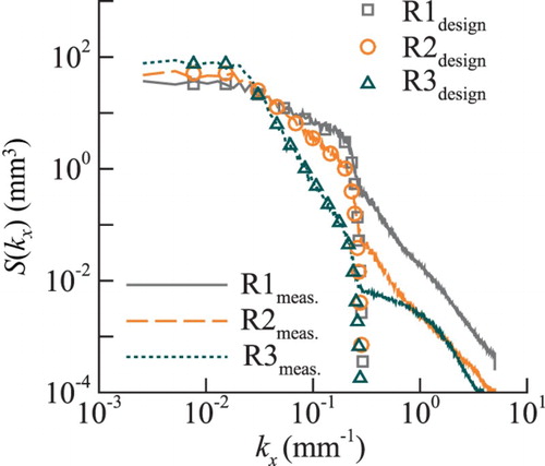
The final column in Table 1 lists values of $\beta$, which were estimated by fitting a regression line through the measured wavenumber spectra $S\left(k_x\right)$ in the scaling region. Corresponding plots of $S\left(k_x\right)$ are shown in Fig. 4. Overall agreement between the measured profiles of the manufactured roughness tiles and the original design spectrum (Eq. (14)) is very good, in terms of both the magnitude of the spectral exponent as well as the limits of the scaling region.

Figure 4 Wavenumber spectra computed using the measured bed profiles (lines) compared to the design spectra of Eq. (14) (symbols)

Hydraulic conditions in the AOCF flume experiments

The ranges of the key hydraulic parameters covered in the AOCF experiments are presented in Table 2, while full sets of experimental data are provided in the online Supplementary Material (Tables S1–S9). Three bed slopes (0.1%, 0.2% and 0.3%) were selected for experiments with each roughness type and for a given bed slope, while the relative submergence was varied as widely as possible within the capabilities of the facility. During every experiment, the flow rate $Q$ was estimated from 30 min recordings of the flowmeter output. Throughout this time 15 longitudinal scans of the water surface elevation were carried out between $x$ = 3.5 m and $x$ = 17.5 m using a confocal sensor (IFS2405-10 sensor and IFC2451 controller by Micro-Epsilon, Birkenhead, UK) attached to the three-axis stage. Individual scans were distributed symmetrically about the channel centreline with 20 mm transverse spacing. The confocal sensor traversed the water surface at 250 mm·s⁻¹ and sampled at 1000 Hz.

Table 2 Ranges of key hydraulic parameters

$S\left(\mathrm{\%}\right)$	$H$(mm)	$U$(m s^−1)	$B/H$(–)	$H/\mathrm{\Delta }$(–)	$\text{F}$ (–)	$\text{R}$(–)	${\mathrm{\Delta }}^{+}$ (–)
0.1	30–160	0.13–0.49	3.3–39.0	5.0–27.0	0.24–0.44	3900–78,400	90–208
0.2	25–140	0.16–0.65	4.0–46.9	4.2–23.4	0.32–0.60	4000–91,000	114–273
0.3	20–120	0.17–0.79	4.4–62.5	3.1–20.1	0.36–0.73	3400–94,800	125–312

Notes: $S$ is the mean water surface slope; $H$ is the mean flow depth; $U=Q/BH$ is the bulk velocity, $Q$ is the volumetric flowrate and $B$ is the flume width; $B/H$ is the aspect ratio; $H/\mathrm{\Delta }$ is the relative submergence and $\mathrm{\Delta }=4{\sigma }_z$ is the roughness height; $\text{F}=U/(gH{)}^{0.5}$ is the Froude number; $\text{R}=UH/\nu$ is the bulk Reynolds number and $\nu$ is the kinematic viscosity; ${\mathrm{\Delta }}^{+}=\mathrm{\Delta }{u}_{\ast }/\nu$ is the roughness Reynolds number and $u\ast =(gSH{)}^{0.5}$ is the shear velocity.

Flow depth $H\left(x\right)$ along the flume was calculated for every experiment as the distance between the mean water surface elevation and the mean rough bed level (mean values were obtained by averaging 15 scans of the water surface and 60 scans of the bed elevation). Flow uniformity was established by ensuring that the gradient of a regression line through $H\left(x\right)$ between $x$ = 3.5 m and $x$ = 15 m was within the range ±5.4E-05. The downstream limit of $x$ = 15 m was chosen to minimize the influence of exit effects occurring in the proximity of the weir. The mean flow depth $H$ listed in Tables S1–S9 was then estimated as the average of $H\left(x\right)$ between $x$ = 3.5 m and $x$ = 15 m. The parameter $S$ in Tables S1–S9 is the mean water surface slope, estimated as the gradient of a linear regression line fitted through the mean water surface profile between $x$ = 3.5 m and $x$ = 15 m. The mean water surface profile was calculated as the difference between the mean water surface elevation and a corresponding stationary water surface profile. The stationary water surface profiles were measured for each of the three bed slopes. The streamwise extent, carriage velocity and sampling frequency of the stationary water surface scans were identical to the water surface elevation scans discussed above.

4.2 Experiments in a narrow open-channel flume

RS flume

A second set of friction factor measurements were carried out in the Fluid Mechanics Laboratory at the University of Aberdeen using a narrow open-channel flume, denoted hereafter as the RS flume (e.g. Manes, Pokrajac, Nikora, Ridolfi, & Poggi, 2011). The RS flume is 0.4 m wide and has a working length of 11.5 m. It utilizes honeycomb mesh and stainless steel vanes in the entrance tank to ensure homogenous, two-dimensional flow at the channel inlet and has a vertical slat weir mechanism at the exit to moderate the backwater profile. A single variable frequency centrifugal pump circulates water through the flume, while an electromagnetic flowmeter records the flow rate. Similar to the AOCF flume, the RS flume sidewalls are constructed from glass panels. The roughness plates were installed in the RS flume in a 29 × 1 array and were fixed in position using a “hook and loop fastener” system.

Hydraulic conditions in the RS flume

The ranges of the key hydraulic parameters covered in the RS flume experiments are presented in Table 2. Full sets of experimental data are provided in the online Supplementary Material (Tables S10–S18). The bed slope and relative submergence values were chosen to match those measured in the AOCF flume as closely as possible. Furthermore, since the RS flume lacked the scanning capability of the AOCF, the parameters $H$ and $S$ were estimated in a different manner. During each experiment, the flow rate was recorded and uniform flow conditions were established and controlled by measuring the water depth using 10 rulers which were attached to the flume sidewall at 1 m intervals along the channel. The glass sidewalls in the flume were coated with a hydrophobic spray that removed the meniscus effect to improve the accuracy of readings from the rulers. The mean flow depth $H$ given in Tables S10–S18 was then calculated by averaging eight out of the 10 readings, neglecting the first and last locations to avoid potential errors introduced by entrance and exit effects. The mean water surface slope $S$, which is listed in Tables S10–S18, was estimated as the gradient of a regression line fitted through the mean water surface profile, excluding 1 m long sections adjacent to the flume entrance and exit. The mean water surface profile was calculated as the difference between the running water surface profile and a corresponding stationary water surface profile. Water surface profile measurements were made along the channel centreline at 500 mm intervals using a point gauge.

5 Results

5.1 Influence of relative submergence on the friction factor

All measured friction factor data collected from the AOCF and RS flumes are plotted as a function of $H/\mathrm{\Delta }$ in Fig. 5. A greater divergence between $(8/f_H{)}^{0.5}$ and $(8/f_R{)}^{0.5}$ is seen in the narrower RS flume as $H/\mathrm{\Delta }$ increases, reflecting the growing contribution to $f_R$ from the smooth sidewalls relative to the wider AOCF flume. The results also demonstrate that $(8/f_R{)}^{0.5}$ is better described as a power law, while $(8/f_H{)}^{0.5}$ displays excellent agreement with a semi-logarithmic fit. Coefficients of these least squares fits to the data in Fig. 5 are summarized in Tables 3 and 4, respectively. The true but unknown bed friction factor $f_b$ exists between these limits, as previously indicated by Eq. (11). However, we can infer changes to $f_b$ indirectly by exploring related trends in $f_H$ and $f_R$. Several points are worth mentioning. Firstly, the current data seem to show the same behaviour across the full range of measured $H/\Delta$, including fairly low submergence (Table 2). This is perhaps somewhat unexpected since several researchers have suggested modifications to the resistance laws at low submergence (e.g. Ferguson, 2007; Katul, Wiberg, Albertson, & Hornberger, 2002; Nikora, Goring, McEwan, & Griffiths, 2001). The lack of the expected trend change at low submergence may be due to insufficient coverage of this range of $H/\mathrm{\Delta }$ but may also reflect some physical reasons which are worth exploring. Secondly, to check the trends of the upper limit of $f_b$ we employed Eq. (2) where instead of the hydraulic radius we use the flow depth. The values of $m_1$ in Eq. (2), listed in Table 3, are seen to vary not only between the AOCF flume and the RS flume but also between R1, R2 and R3. While the difference between R2 and R3 is within uncertainty limits (Table 3), it is significantly higher for R1. Thirdly, the value of the offset $c_1$ (Eq. (2)) given in Table 3 systematically increases as $\beta$ increases. This suggests that hydraulic resistance is decreasing as $\beta$ increases from 1 to 3, thus revealing an important effect of the spectral structure of the bed. Similar systematic variations are observed in the power law relationships summarized in Table 4, i.e. the lower limit of $f_b$. Such changes in $f_H$ and $f_R$, and therefore in $f_b$, reflect underlying modifications in the velocity field caused by an interplay of bed roughness structure, relative submergence, and channel aspect ratio effects. Additional experiments are needed though to elucidate these findings. However, the aforementioned points do clearly highlight a potential shortfall of traditional hydraulic resistance formulae built around single characteristic roughness lengths and demonstrate that additional roughness metrics, in this case the spectral exponent, are needed to better determine hydraulic behaviour.

Figure 5 Friction factor plotted as a function of $H/\mathrm{\Delta }$. Symbol key: □ $S=0.1\mathrm{\%}$; ◊ $S=0.2\mathrm{\%}$; ○ $S=0.3\mathrm{\%}$; closed, $f_H$; open, $f_R$; green, AOCF flume; orange, RS flume. Solid (dashed) lines show logarithmic (power) fits to the data, the coefficients of the fits are summarized in Table 3 (Table 4)

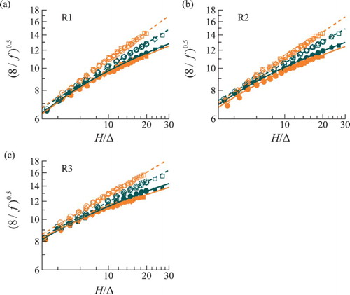
Table 3 Summary of the friction factor relationships of the form $(8/f_H{)}^{0.5}=m_1\ln \left(H/\mathrm{\Delta }\right)+c_1$ fitted to the measured data in Fig. 5

Flume	Roughness	$\beta$	$m_1$	$c_1$	$N_s$	$R^2$
AOCF	R1	1	2.80 ± 0.03	3.29 ± 0.07	39	0.999
	R2	5/3	2.62 ± 0.03	4.05 ± 0.07	39	0.999
	R3	3	2.69 ± 0.07	5.20 ± 0.18	38	0.994
RS	R1	1	2.69 ± 0.08	3.35 ± 0.18	47	0.991
	R2	5/3	2.48 ± 0.08	4.02 ± 0.18	50	0.989
	R3	3	2.38 ± 0.09	5.70 ± 0.21	44	0.985

Notes: $N_s$ is the number of data points used in the least squares regression, $R^2$ is the coefficient of determination of the least squares regression.

Table 4 Summary of the friction factor relationships of the form $(8/f_R{)}^{0.5}=c_2(H/\mathrm{\Delta }{)}^{m_2}$ fitted to the measured data in Fig. 5

Flume	Roughness	$\beta$	$m_2$	$c_2$	$N_s$	$R^2$
AOCF	R1	1	0.344 ± 0.007	1.524 ± 0.017	39	0.996
	R2	5/3	0.313 ± 0.004	1.631 ± 0.019	39	0.999
	R3	3	0.290 ± 0.007	1.812 ± 0.016	38	0.995
RS	R1	1	0.403 ± 0.008	1.460 ± 0.018	47	0.996
	R2	5/3	0.376 ± 0.009	1.542 ± 0.021	50	0.994
	R3	3	0.330 ± 0.007	1.789 ± 0.017	44	0.995

5.2 Effect of the spectral exponent on the friction factor

A further understanding of the effect of the spectral exponent is illustrated in Fig. 6. These plots compare flows with matched $S$ and $H/\mathrm{\Delta }$ values but different roughness types and so directly isolate the effect of the spectral exponent. Dashed lines in the plots indicate linear least squares fits to the data of the form ${f_H}_{(\beta =y)}=m_3{f_H}_{(\beta =x)}$ with $m_3$ as a numerical constant. Here we consider only fits to $f_H$ for brevity but note that results for $f_R$ and hence $f_b$ are similar. Indeed, the differences in fitting lines for $f_H$ and $f_R$ would hardly be distinguishable visually. Full details about the linear relationships are contained in Table 5. Figure 6 confirms the previous observation that friction factor decreases from a maximum when $\beta$ = 1 to a minimum when $\beta$ = 3. This difference is as high as 49% when comparing the R1 and R3 beds (Fig. 6c), suggesting that the features of the scaling range of bed roughness make a key contribution to the bed hydraulic resistance. This finding appears to be insensitive to the aspect ratio of the channel as evidenced by the close agreement between results from the AOCF and RS flumes.

Figure 6 Effect of the spectral exponent on the friction factor. Symbol key: closed, $f_H$; open, $f_R$; green, AOCF flume; orange, RS flume. The dash-dot line shows $f_{(\beta =y)}=f_{(\beta =x)}$ while the dashed green (orange) line is a linear least squares fit through the $f_H$ data points from the AOCF flume (RS flume) with the offset forced to zero. The coefficients of the linear fits are summarized in Table 5

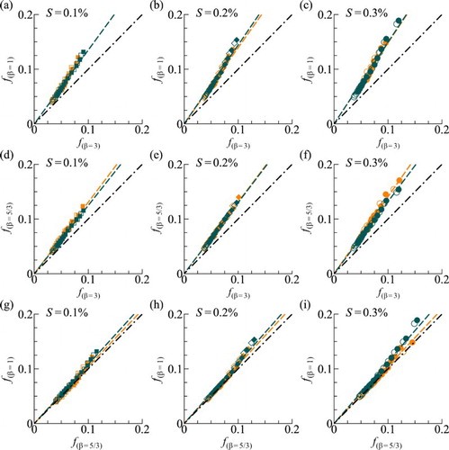
Table 5 Summary of linear least squares relationships of the form $f_{H(\beta =y)}=m_3{f}_{H(\beta =x)}$ fitted to the measured data in Fig. 6

			AOCF flume			RS flume
$x$	$y$	$S\left(\mathrm{\%}\right)$	$m_3$	$N_s$	$R^2$	$m_3$	$N_s$	$R^2$
5/3	1	0.1	1.08 ± 0.02	13	0.985	1.04 ± 0.03	18	0.914
5/3	1	0.2	1.11 ± 0.03	13	0.976	1.05 ± 0.03	15	0.951
5/3	1	0.3	1.13 ± 0.04	13	0.969	1.07 ± 0.02	14	0.975
3	5/3	0.1	1.25 ± 0.02	13	0.994	1.31 ± 0.02	18	0.961
3	5/3	0.2	1.30 ± 0.02	12	0.990	1.31 ± 0.02	15	0.976
3	5/3	0.3	1.32 ± 0.02	13	0.994	1.41 ± 0.04	11	0.969
3	1	0.1	1.35 ± 0.04	13	0.967	1.35 ± 0.04	17	0.849
3	1	0.2	1.44 ± 0.06	12	0.934	1.39 ± 0.04	14	0.906
3	1	0.3	1.49 ± 0.06	13	0.961	1.48 ± 0.06	10	0.877

Looking at the values of $m_3$ in Table 5 there is an apparent effect of the channel bed slope. For example, when comparing the R1 and R3 beds in the AOCF the constant $m_3$ increases from 1.35 to 1.49 as $S$ increases from 0.1% to 0.3%. This is somewhat unexpected since no effects of $S$ were visible from the results in Fig. 5. Bathurst (1985) comments on the possible indirect influence of bed slope on flow resistance through the Froude number and associated free surface disturbances. However, standard deviation estimates of the free surface fluctuations (not shown) indicate that in our experiments the largest free surface disturbances occur over the R3 bed, in direct contrast to the observed trends. Aberle and Smart (2003) also reported a dependence of the flow resistance factors on bed slope, albeit for much steeper channels comprised of complex step-pool geometries, such that different physical mechanisms are expected to be responsible for the variations that they observe. Here it is noted that the majority of changes in $m_3$ are within the limits of uncertainty (Table 5) and subsequently a definite trend cannot be firmly claimed. Measurements over a wider range of bed slopes are required to clarify these initial findings.

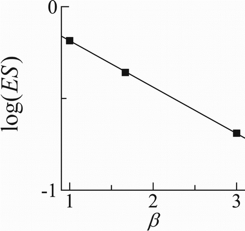
5.3 Relationship between the spectral model and effective bed roughness slope

The observations from Figs 5 and 6 are in line with previous studies that have reported an increase in the Hama roughness function $\mathrm{\Delta }{U}^{+}$ (Hama, 1954) when increasing the effective slope ($ES$) of the bed roughness while keeping the roughness height fixed (e.g. Chan, MacDonald, Chung, Hutchins, & Ooi, 2015; Napoli, Armenio, & De Marchis, 2008; Schultz & Flack, 2009). To characterize the surface roughness, Napoli et al. (2008) introduced $ES$, which can be defined for two-dimensional surfaces as: (19) $ES=\frac{1}{L_x}\frac{1}{L_y}{\int }_0^{L_y}{\int }_0^{L_x}\left|\frac{\mathrm{\partial }z(x,y)}{\mathrm{\partial }x}\right|dxdy$(19) where L_x, L_y are the longitudinal and transverse lengths of the roughness patterns, respectively. Here we briefly consider how $ES$ is connected with $\beta$ in the context of our spectral model of bed roughness. We start by noting that the power spectrum of the streamwise gradient of the bed elevations is given by $(2\pi {)}^{2}S\left(k_x\right)k_x^2$, recalling that we define the streamwise wavenumber as $k_x=1/\lambda$, where $\lambda$ is wavelength. Integrating $(2\pi {)}^{2}S\left(k_x\right)k_x^2$ yields the variance of $\mathrm{\partial }z(x,y)/\mathrm{\partial }x$ which can then be linked to $ES$ as follows: (20) $ES=2\pi {\left(\frac{2}{\pi }{\int }_0^{\mathrm{\infty }}S\left(k_x\right)k_x^{2}d{k}_x\right)}^{1/2}$(20) where the constant $(2/\pi {)}^{1/2}$ in Eq. (20) strictly applies only if the bed roughness elevations obey a Gaussian distribution.

As Eq. (20) shows, the parameter $ES$ depends on the spectra of bed elevations. In the case of our model, it depends on $k_{c1}$, $k_{c2}$, ${\sigma }_z$ and $\beta$. However, since the parameters $k_{c1}$, $k_{c2}$ and ${\sigma }_z$ are the same for R1, R2, and R3, we can examine the direct relationship between $ES$ and $\beta$. This is illustrated in Fig. 7 where the gradient of the bed elevations is seen to increase as $\beta$ decreases, in agreement with an approximate relation $\log \left(ES\right)=c-m\beta$ that follows from Eq. (20) and our spectral model in Fig. 1 (note that constants $c$ and $m$ depend on $k_{c1}$, $k_{c2}$, and ${\sigma }_z$). The higher flow resistance observed at $\beta =1$ (Figs Figs 5 and 6) can then reasonably be linked, at least in part, to an associated rise in the steepness of the bed elevations (Fig. 7) which in turn would cause a heightened occurrence of local flow separation and enhanced pressure (form) drag.

Figure 7 Effective slope as a function of $\beta$ for $k_{c1}=0.02$ mm⁻¹, $k_{c2}=0.2$ mm⁻¹ and ${\sigma }_z=1.5$ mm

As an additional point, we note here the consistency with the results of Chan et al. (2015) who found a relation between $ES$ and $\mathrm{\Delta }{U}^{+}$ of the form: (21) $\mathrm{\Delta }{U}^{+}=\frac{1}{\kappa }\log \left(\frac{k_a{u}_{\ast }}{\nu }\right)+1.12\log \left(ES\right)+1.47$(21) where $\kappa$ is the von Kármán constant and $k_a$ is the average roughness height. For a fixed value of $k_a$, the approximate relation in Fig. 7 can be combined with Eq. (21) leading to the following expression linking $\mathrm{\Delta }{U}^{+}$ and $\beta$: (22) $\mathrm{\Delta }{U}^{+}=\text{{X}}-1.12m\beta$(22) where $\text{{X}}$ and $m$ are constants dependent on model roughness parameters, as noted above. The validity of Eq. (22) remains to be tested however.

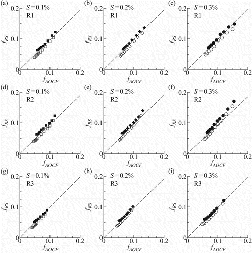
5.4 Effect of aspect ratio on the friction factor

The dimensions of the roughness plates and the widths of the open-channel flumes used in these experiments afforded an opportunity to investigate the effects of channel aspect ratio on the friction factor. For instance, matching the mean flow depth and bed slope between the RS and the AOCF flumes yielded flows with near identical ${\mathrm{\Delta }}^{+}$ and $H/\mathrm{\Delta }$ but with aspect ratios which differed by a factor of approximately 3. Figure 8 directly compares measured friction factor values between the AOCF and RS flumes at the same $S$ and $H/\mathrm{\Delta }$ values to highlight any changes resulting from differences in $B/H$. The dashed lines in the plots indicate $f_{RS}=f_{AOCF}$. In general, $f_H$ and $f_R$ are seen to fall either side of the $f_{RS}=f_{AOCF}$ line, particularly for high aspect ratios (lowest values of $f_H$ and $f_R$), implying that $f_b$ follows the $f_{RS}=f_{AOCF}$ line closely. This type of behaviour is expected, if no effects of $B/H$ on $f_b$ are assumed. Some scatter in the results is visible at low aspect ratios but no systematic trends are apparent, indicating that the discrepancies are more likely related to increased measurement uncertainties associated with the shallowest flows. The results in Fig. 8 reflect the fact that $f_b$ is a bulk coefficient, based on the cross-sectionally averaged bed shear stress ${\overline{\tau }}_b$. Therefore, while local fluctuations in ${\tau }_b$ will arise due to the effect of secondary currents (e.g. Nezu & Nakagawa, 1993), when comparing ${\overline{\tau }}_b$ at different $B/H$ these effects tend to be averaged out. This matter, however, needs a wider range of the aspect ratio to be firmly resolved.

Figure 8 Effect of the channel aspect ratio on the friction factor. Symbol key: closed, $f_H$; open, $f_R$. The dash-dot line shows $f_{RS}=f_{AOCF}$

6 Conclusions

A set of experiments were carried out in two separate open-channel facilities to investigate the effects of bed roughness structure, flow submergence, and channel aspect ratio on hydraulic resistance. Three different self-affine surfaces were tested, each with identical statistical properties ($k_{c1}$, $k_{c2}$ and ${\sigma }_z$) but with different spectral exponents of $\beta$ = 1, 5/3, and 3, respectively. The numerical design and physical manufacture of these self-affine roughness patterns was described. Longitudinal scans of the bed roughness installed in the AOCF flume verified the validity of the design and manufacturing process. The spectral exponent of the bed roughness was seen to play an important role in modifying hydraulic resistance. The results show that with all else equal, decreasing the spectral exponent of the bed roughness leads to a subsequent increase in the friction factor. This difference was observed to be as great as 49% between the R1 and R3 beds and was ascertained independently of channel aspect ratio. A link between $\beta$ and $ES$ was illustrated analytically and with the data, showing $ES$ increasing as $\beta$ decreases and suggesting that increased flow separation around steeper, scaling-range roughness features makes a key contribution to the overall resistance. The dimensions of the roughness plates and the widths of the open-channel flumes used in these experiments afforded an opportunity to investigate channel aspect ratio effects. No influence of the aspect ratio on $f_b$ was apparent from the results however, even though $B/H$ differed by a factor of 3 between the RS and AOCF flumes.

Looking forward, the spectral synthesis approach is deemed to be particularly beneficial for the systematic study of multi-scale rough-bed flows since it allows strict control over the statistical properties of the surface and thus offers the possibility for better repeatability and comparability between experiments in different facilities as well as numerical simulations. Indeed, while the present manuscript focused primarily on hydraulic resistance, future work will involve more detailed velocity field exploration using data collected through stereoscopic PIV in combination with LES. A particular area of focus will be to quantify contributions from constituent components of the friction factor, following the decomposition proposed by Nikora (2009).

Supplemental data

Supplemental data for this article can be accessed here https://doi.org/10.1080/00221686.2018.1473296.

Notation
$a_1,a_2$	=	numerical constants (–)
$A$	=	channel cross-sectional area (m2)
$A_{surf}$	=	total wetted surface area (m2)
$B$	=	channel width (m)
$B/H$	=	aspect ratio (–)
$c,c_1,c_2$	=	numerical constants (–)
$C$	=	Chézy coefficient (m1/2 s−1)
$ES$	=	effective slope of bed roughness (–)
$f_b,f_H,f_R$	=	friction factor based on mean bed shear stress, flow depth and hydraulic radius (–)
$\mathsf{F}$	=	Froude number (–)
$g$	=	gravity acceleration (m s−2)
$H$	=	mean flow depth (mm)
$H/\mathrm{\Delta }$	=	relative submergence based on mean flow depth (–)
$j$	=	imaginary unit (–)
$k_a$	=	average roughness height (mm)
$k_{c1},k_{c2}$	=	low and high wavenumber cut-offs in the design spectrum (mm−1)
$k_r$	=	radial wavenumber (mm−1)
$k_x,k_y$	=	streamwise and transverse wavenumbers (mm−1)
$K{u}_z$	=	Kurtosis of bed elevations (–)
$l_x,l_y$	=	longitudinal and transverse roughness lengths (mm)
$L$	=	section length along the channel (m)
$L_x,L_y$	=	streamwise and transverse lengths of the bed roughness (mm)
$m,m_1,m_2,m_3$	=	numerical constants (–)
$P$	=	wetted perimeter
$Q$	=	volumetric flow rate (m s−3)
$\mathsf{R}$	=	bulk Reynolds number (–)
$R$	=	hydraulic radius (m)
$R/\mathrm{\Delta }$	=	relative submergence based on hydraulic radius (–)
$R^2$	=	coefficient of determination (–)
$n$	=	Manning’s roughness coefficient (m−1/3 s)
$N$	=	number of discrete grid points (–)
$N_s$	=	number of samples in least squares regression (–)
$N_{eff}$	=	number of independent samples (–)
$S$	=	mean water surface slope (–)
$S_b$	=	channel bed slope (–)
$S\left(\mathit{k}\right)$	=	two-dimensional wavenumber spectra of bed elevations (mm4)
$S\left(k_x\right)$	=	one-dimensional streamwise wavenumber spectra of bed elevations (mm3)
$S{k}_z$	=	Skewness of bed elevations (–)
$u_{\ast }$	=	shear velocity (m s−1)
$U$	=	bulk velocity (m s−1)
$x,y,z$	=	streamwise, transverse and vertical coordinates (–)
$\text{z}\left(\mathit{x}\right)$	=	height field in spatial domain (mm)
$z_{sb}(x,y)$, $z_{rb}(x,y)$, $z_b(x,y)$	=	smooth, rough and corrected rough bed elevation profiles (mm)
$Z\left(\mathit{k}\right)$	=	height field in wavenumber domain (mm)
$\alpha$	=	Hurst exponent (–)
$\beta$	=	spectral exponent (–)
${\chi }_{N_{eff}-1;\gamma /2}^2$	=	chi-squared distribution with $N_{eff}-1$ degrees of freedom at $\gamma$ confidence level
$\text{{X}}$	=	numerical constant
$\mathrm{\Delta }$	=	roughness height (m)
${\mathrm{\Delta }}_x,{\mathrm{\Delta }}_y$	=	streamwise and transverse grid spacing in spatial domain (mm)
${\mathrm{\Delta }}_{kx},{\mathrm{\Delta }}_{ky}$	=	streamwise and transverse grid spacing in wavenumber domain (mm−1)
${\mathrm{\Delta }}^{+}$	=	roughness Reynolds number (–)
$\mathrm{\Delta }{U}^{+}$	=	Hama (1954) roughness function (–)
$\lambda$	=	wavelength (mm)
$\nu$	=	kinematic viscosity (m2 s−1)
$\rho$	=	fluid density (kg m−3)
${\sigma }_z$	=	standard deviation of bed elevations (mm)
${\tau }_0$	=	total surface shear stress (Pa)
${\overline{\tau }}_0,{\overline{\tau }}_b,{\overline{\tau }}_w$	=	mean surface, bed and sidewall shear stress (Pa)

Acknowledgements

The authors wish to express their gratitude to Stephan Spiller for advice regarding the silicone moulds, to Cameron Scott for assisting with manufacturing of the roughness elements and Davide Collautti for help with conducting experiments.

ORCID

Vladimir I. Nikora http://orcid.org/0000-0003-1241-2371

Ivan Marusic http://orcid.org/0000-0003-2700-8435

Additional information

Funding

Financial support was provided by the Engineering and Physical Sciences Research Council [grant EP/K041088/1]. IM acknowledges the support of the Australian Research Council [grant FL120100017].

References

- Aberle, J., & Smart, G. M. (2003). The influence of roughness structure on flow resistance on steep slopes. Journal of Hydraulic Research, 41(3), 259–269. doi: 10.1080/00221680309499971
- Anderson, W., & Meneveau, C. (2011). Dynamic roughness model for large-eddy simulation of turbulent flow over multiscale fractal-like rough surfaces. Journal of Fluid Mechanics, 679, 288–314. doi: 10.1017/jfm.2011.137
- Barros, J., Schultz, M., & Flack, K. (2015). Skin-friction measurements on mathematically generated roughness in a turbulent channel flow. Bulletin of the American Physical Society, 60.
- Bathurst, J. C. (1985). Flow resistance estimation in mountain rivers. Journal of Hydraulic Engineering, 111(4), 625–643. doi: 10.1061/(ASCE)0733-9429(1985)111:4(625)
- Bathurst, J. C. (2002). At-a-site variation and minimum flow resistance for mountain rivers. Journal of Hydrology, 269(1), 11–26. doi: 10.1016/S0022-1694(02)00191-9
- Bell, T. H. (1975). Statistical features of sea-floor topography. Deep Sea Research and Oceanographic Abstracts, 22(12), 883–892. doi: 10.1016/0011-7471(75)90090-X
- Bendat, J. & Piersol, A. (2010). Random data: Analysis and measurement procedures (4th ed.). Hoboken, NJ: Wiley.
- Butler, J. B., Lane, S. N., & Chandler, J. H. (2001). Characterization of the structure of river-bed gravels using two-dimensional fractal analysis. Mathematical Geology, 33(3), 301–330. doi: 10.1023/A:1007686206695
- Cameron, S. M., Nikora, V. I., & Stewart, M. T. (2017). Very-large-scale motions in rough-bed open-channel flow. Journal of Fluid Mechanics, 814, 416–429. doi: 10.1017/jfm.2017.24
- Chan, L., MacDonald, M., Chung, D., Hutchins, N., & Ooi, A. (2015). A systematic investigation of roughness height and wavelength in turbulent pipe flow in the transitionally rough regime. Journal of Fluid Mechanics, 771, 743–777. doi: 10.1017/jfm.2015.172
- Einstein, H. (1942). Formulas for the transportation of bed load. Transactions of ASCE, 107, 561–597.
- Ferguson, R. (2007). Flow resistance equations for gravel- and boulder-bed streams. Water Resources Research, 43(5), 259. doi: 10.1029/2006WR005422
- Flack, K. A., & Schultz, M. P. (2010). Review of hydraulic roughness scales in the fully rough regime. Journal of Fluids Engineering, 132(4), 041203. doi: 10.1115/1.4001492
- Grinvald, D. I., & Nikora, V. (1988). Rechnaya turbulentsiya [ River Turbulence]. Leningrad: Hydrometeo-Izdat.
- Hama, F. (1954). Boundary-layer characteristics for rough and smooth surfaces. Transactions-Society of Naval Architects and Marine Engineers, 62, 333.
- Hino, M. (1968). Equilibrium-range spectra of sand waves formed by flowing water. Journal of Fluid Mechanics, 34(3), 565–573. doi: 10.1017/S0022112068002089
- Hubbard, B., Siegert, M. J., & McCarroll, D. (2000). Spectral roughness of glaciated bedrock geomorphic surfaces: Implications for glacier sliding. Journal of Geophysical Research: Solid Earth, 105(B9), 21295–21303. doi: 10.1029/2000JB900162
- Hurst, H. (1951). Long-term storage capacity of reservoirs. Transaction of the American Society of Civil Engineers, 116, 770–808.
- Katul, G., Wiberg, P., Albertson, J., & Hornberger, G. (2002). A mixing layer theory for flow resistance in shallow streams. Water Resources Research, 38(11), 32-1–32-8. doi: 10.1029/2001WR000817
- Keulegan, G. H. (1938). Laws of turbulent flow in open channels. Journal of Research of the National Bureau of Standards, 21, 707–741. doi: 10.6028/jres.021.039
- Knight, D. W., Demetriou, J. D., & Hamed, M. E. (1984). Boundary shear in smooth rectangular channels. Journal of Hydraulic Engineering, 110(4), 405–422. doi: 10.1061/(ASCE)0733-9429(1984)110:4(405)
- Lee, A. J., & Ferguson, R. I. (2002). Velocity and flow resistance in step-pool streams. Geomorphology, 46(1), 59–71. doi: 10.1016/S0169-555X(02)00054-5
- Majumdar, A., & Tien, C. L. (1990). Fractal characterization and simulation of rough surfaces. Wear, 136(2), 313–327. doi: 10.1016/0043-1648(90)90154-3
- Manes, C., Pokrajac, D., Nikora, V. I., Ridolfi, L., & Poggi, D. (2011). Turbulent friction in flows over permeable walls. Geophysical Research Letters, 38(3). doi: 10.1029/2010GL045695
- Mankoff, K., Gulley, J., Tulaczyk, S., Covington, M., Liu, X., Chen, Y., … Głowacki, P. (2017). Roughness of a subglacial conduit under Hansbreen, Svalbard. Journal of Glaciology, 63(239), 423–435. doi: 10.1017/jog.2016.134
- Napoli, E., Armenio, V., & De Marchis, M. (2008). The effect of the slope of irregularly distributed roughness elements on turbulent wall-bounded flows. Journal of Fluid Mechanics, 613, 385–394. doi: 10.1017/S0022112008003571
- Nezu, I., & Nakagawa, H. (1993). Turbulence in open channel flows. Rotterdam: A. A. Balkema.
- Nikora, V. (2009, August). Friction factor for rough-bed flows: Interplay of fluid stresses, secondary currents, non-uniformity, and unsteadiness. Proceedings, 33rd IAHR Congress (p. 1246). Vancouver, Canada. Vol. 10, No. 14.
- Nikora, V., & Goring, D. (2004). Mars topography: Bulk statistics and spectral scaling. Chaos, Solitons & Fractals, 19(2), 427–439. doi: 10.1016/S0960-0779(03)00054-7
- Nikora, V., Goring, D., McEwan, I., & Griffiths, G. (2001). Spatially averaged open-channel flow over rough bed. Journal of Hydraulic Engineering, 127(2), 123–133. doi: 10.1061/(ASCE)0733-9429(2001)127:2(123)
- Nikora, V. I., Goring, D. G., & Biggs, B. J. F. (1998). On gravel-bed roughness characterization. Water Resources Research, 34(3), 517–527. doi: 10.1029/97WR02886
- Nikora, V. I., Sukhodolov, A. N., & Rowinski, P. M. (1997). Statistical sand wave dynamics in one-directional water flows. Journal of Fluid Mechanics, 351, 17–39. doi: 10.1017/S0022112097006708
- Nikuradse, J. (1933). Strömungsgesetze in rauhen Rohren. Forschung auf dem Gebiete des Ingenieurwesens, Forschungsheft 361, VDI Verlag, Berlin, Germany (in German) (English translation: Laws of flow in rough pipes, NACA Technical Memorandum 1292, 1950).
- Saupe, D. (1988). Algorithms for random fractals. In H.-O. Peitgen & D. Saupe (Eds.), The science of fractal images (pp. 71–136). New York, NY: Springer-Verlag.
- Schlichting, H. (1979). Boundary-layer theory. New York, NY: McGraw-Hill.
- Schultz, M. P., & Flack, K. A. (2009). Turbulent boundary layers on a systematically varied rough wall. Physics of Fluids, 21(1), 015104. doi: 10.1063/1.3059630
- Singh, A., Porté-Agel, F., & Foufoula-Georgiou, E. (2010). On the influence of gravel bed dynamics on velocity power spectra. Water Resources Research, 46(4), 117. doi: 10.1029/2009WR008190
- Smart, G. M., Duncan, M. J., & Walsh, J. M. (2002). Relatively rough flow resistance equations. Journal of Hydraulic Engineering, 128(6), 568–578. doi: 10.1061/(ASCE)0733-9429(2002)128:6(568)
- Turcotte, D. (1997). Fractals and chaos in geology and geophysics (2nd ed.). New York, NY: Cambridge University Press.
- Vanoni, V., & Brooks, N. (1957). Laboratory studies of the roughness and suspended load of alluvial streams (Report No. E-68). Pasadena, CA.