
 ?Mathematical formulae have been encoded as MathML and are displayed in this HTML version using MathJax in order to improve their display. Uncheck the box to turn MathJax off. This feature requires Javascript. Click on a formula to zoom.
ABSTRACT
Flow resistance due to vegetation is of interest for a wide variety of hydraulic engineering applications. This note evaluates several practical engineering functions for estimating bulk drag coefficient () for arrays of rigid cylinders, which are commonly used to represent emergent vegetation. Many of the evaluated functions are based on an Ergun-derived expression that relates
to two coefficients, describing viscous and inertial effects. A re-parametrization of the Ergun coefficients based on cylinder diameter (d) and solid volume fraction (φ) is presented. Estimates of
are compared to a range of experimental data from previous studies. All functions reasonably estimate
at low φ and high cylinder Reynolds numbers (
). At higher φ they typically underestimate
. Estimates of
utilizing the re-parametrization presented here match the experimental data better than estimates of
made using the other functions evaluated, particularly at low φ and low
.
1 Introduction
Vegetation occurs in many natural and engineered water systems (O'Hare, Citation2015). In rivers the additional drag caused by vegetation acts to increase flow depths, potentially increasing the risk of flooding (Darby, Citation1999). In stormwater ponds, the resistance of vegetation has a dominant impact on the flow field and therefore affects treatment potential (Sonnenwald, Guymer, & Stovin, Citation2017). Determining vegetation drag is therefore of interest for a range of hydraulic engineering applications.
1.1 Existing measurements of 
Arrays of rigid cylinders are often used to represent emergent vegetation, e.g. Bennett, Pirim, and Barkdoll (Citation2002), Nepf (Citation1999), Rameshwaran and Shiono (Citation2007), Rowiński and Kubrak (Citation2002), Serra, Fernando, and Rodríguez (Citation2004), Tanino and Nepf (Citation2008b) and Tinoco and Cowen (Citation2013). Table presents seven datasets where the bulk drag coefficient, , for emergent cylinder arrays has been experimentally or numerically derived. The experimental and numerical methods used for determining
are described below.
Table 1. Summary of experimental data describing drag in arrays of emergent cylinders
Traditionally, is obtained from experimental results for emergent cylinder arrays by equating driving forces with resistance caused by cylinders (Ferreira, Ricardo, & Franca, Citation2009; Kim & Stoesser, Citation2011; Tanino & Nepf, Citation2008a). Assuming wall and bed stresses are negligible, for emergent cylinders this equates to the balance of gravity and drag forces:
(1)
(1) where ρ is density, g is acceleration due to gravity, S is channel or energy slope, φ is solid volume fraction, a is frontal facing area (the cylinder area perpendicular to the direction of flow per unit volume, m2 m−3), and
is mean interstitial velocity (Stone & Shen, Citation2002; Tanino, Citation2012). For cylinders
where d is cylinder diameter. In low velocities or low cylinder densities Eq. (Equation1
(1)
(1) ) is impractical to apply, as it becomes difficult to measure surface slope. Bed and free surface stresses also become more important, eventually invalidating Eq. (Equation1
(1)
(1) ) (Tanino & Nepf, Citation2008a). Instead, drag may be measured directly using a force sensor (Dittrich, Aberle, Schoneboom, Rodi, & Uhlmann, Citation2012; James, Goldbeck, Patini, & Jordanova, Citation2008; Tinoco & Cowen, Citation2013). Measured force is then equated directly with the the right hand side of Eq. (Equation1
(1)
(1) ).
As an alternative to direct measurement, Nepf (Citation1999) assumed that turbulence production in vegetation (arrays of cylinders) is equal to dissipation, that drag dominates energy dissipation, and therefore that turbulence intensity can be equated to drag force as:
(2)
(2) where k is turbulent kinetic energy and
(Tanino & Nepf, Citation2008b). Thus, instantaneous velocity measurements, e.g. from acoustic Doppler velocimetry, may be used to determine k and hence
(Meftah & Mossa, Citation2013).
For simple geometries, such as a single cylinder or periodic arrays of cylinders, may be evaluated using computational fluid dynamics (CFD) tools (Kim & Stoesser, Citation2011; Koch & Ladd, Citation1997; Marjoribanks, Hardy, Lane, & Parsons, Citation2014; Rahman, Karim, & Alim, Citation2007; Stoesser, Kim, & Diplas, Citation2010), either by determining S in Eq. (Equation1
(1)
(1) ) from the streamwise pressure gradient or by extracting the force on a cylinder by integrating the pressure acting on the cylinder wall.
1.2 estimation functions
When no physical measurements are available and CFD-based approaches are infeasible (e.g. a complex geometry) must be estimated. It is well established that
for a single-cylinder is dependent on cylinder Reynolds number
, where
and ν is kinematic viscosity (Schlichting, Gersten, Krause, Oertel, & Mayes, Citation1960; White, Citation1991). For cylinder arrays,
is also dependent on array characteristics (Nepf, Citation1999). Table lists several functions that estimate
depending on array (or vegetation) characteristics. These functions all have a basis in experimental observations and it is of interest to evaluate how successfully they estimate
. The White (Citation1991) function is included as a base comparison.
Table 2. Equations of functions that estimate for arrays of emergent cylinders
The Tanino and Nepf (Citation2008a) and Tinoco and Cowen (Citation2013) functions share a common derivation. Koch and Ladd (Citation1997) showed the Ergun (Citation1952) expression for pressure drop in packed columns to successfully predict drag force. Tanino and Nepf (Citation2008a) related this expression to drag coefficient giving:
(3)
(3) where
and
are coefficients describing viscous and inertial drag effects respectively. Tanino and Nepf (Citation2008a) and Tinoco and Cowen (Citation2013) used their experimental
data to estimate
and
. Linking their values of
and
to the physical characteristics of their cylinder arrays led both to propose linear relationships for predicting
as a function of φ. Tanino and Nepf (Citation2008a) noted that
appeared to be independent of cylinder array characteristics and omitted the viscous term from Eq. (Equation3
(3)
(3) ) in their function estimating
. Tinoco and Cowen (Citation2013) also excluded the viscous component from their function estimating
and suggest it is most suitable at
. Therefore, in both functions
is solely a function of φ.
The similarity of the methods used in the Tanino and Nepf (Citation2008a) and Tinoco and Cowen (Citation2013) studies presents an opportunity to combine their results and create enhanced estimates of from Eq. (Equation3
(3)
(3) ). Sonnenwald, Hart, West, Stovin, and Guymer (Citation2017) re-parametrized
and
in terms of φ and d. The objectives of this note are (i) to improve the re-parametrizations of Sonnenwald et al. (Citation2017) by including additional experimental data; (ii) to demonstrate the validity of these re-parametrizations by comparing estimates of
made using Eq. (Equation3
(3)
(3) ) to experimental data; and (iii) to compare alternative estimates of
with the re-parametrized Eq. (Equation3
(3)
(3) ) and with experimental data.
2 A re-parametrization of the Ergun (Citation1952) coefficients
Figure provides a comparison between values of and
and the corresponding values of φ and d for a range of data. Results from Koch and Ladd (Citation1997) are plotted taking lattice units as mm for comparison purposes.
Figure 1. Plots of the Ergun (Citation1952) coefficients with respect to cylinder array characteristics, (a) vs φ, (b)
vs d, (c)
vs φ, (d)
vs d;
Meftah and Mossa (Citation2013),
![]()
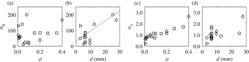
Figure a does not suggest any systematic relationship between and φ, which is consistent with the conclusions of Tanino and Nepf (Citation2008a).
Figure b shows a positive correlation between and d. This is mainly due to the results of Tinoco and Cowen (Citation2013), who varied both φ and d. Tanino and Nepf (Citation2008a), who varied only φ, did not find a relationship with
. It is therefore reasonable to conclude that the variation in
observed by Tinoco and Cowen (Citation2013) is due to d. The results of Koch and Ladd (Citation1997) show a similar trend. Together they suggest a linear relationship between
and d and as a result the data (excluding that of Koch & Ladd, Citation1997) presented in Fig. b have been fit to a linear function, Eq. (Equation4a
(4a)
(4a) ), shown in Fig. b.
Tanino (Citation2012) suggested that viscous drag, the component described by , is proportional to d/s, where s is cylinder spacing. A linear relationship with d is consistent with this. No relationship between
and s (either on its own or with d) was found.
Figure c shows a positive correlation between and φ, which is consistent with both Tanino and Nepf (Citation2008a) and Tinoco and Cowen (Citation2013) who both suggested a linear relationship between
and φ. Tanino (Citation2012) suggested that the inertial drag (described by
) is strongly linked to flow-field heterogeneity, and that φ provides a reasonable estimate of this. Figure d also shows a positive correlation between
and d. A linear relationship between
and d is suggested by the results of Tinoco and Cowen (Citation2013) and Koch and Ladd (Citation1997), similar to
. If
also depends on d, then d may serve to indicate flow-field heterogeneity.
Together, Figs c and d suggest that is a function of both φ and d and all data shown in these two figures (excluding that of Koch & Ladd, Citation1997) have been used to fit a single function (not shown in Fig. ). Combining these two parameters gives a variation in values of
for the same d. Least-squares curve-fitting was undertaken assuming
and
are linear functions giving:
(4a)
(4a)
(4b)
(4b)
where Eq. (Equation4
(4a)
(4a) a) provides an estimate of the viscous effects and Eq. (Equation4
(4a)
(4a) b) provides an estimate of the inertial effects of drag when used in Eq. (Equation3
(3)
(3) ). Note that the coefficients to the d terms must have units m−1 to retain non-dimensionality. Root mean square error (RMSE) values of 38.0 and 0.131 were obtained respectively for
and
. Substituting Eq. (Equation4
(4a)
(4a) ) into Eq. (Equation3
(3)
(3) ) gives a new function for estimating
:
(5)
(5)
3 A comparison of estimates of against experimental results
Figure shows estimates of from the functions in Table and Eq. (Equation5
(5)
(5) ) plotted for a range of
, a representative selection of φ and d, and with the experimental data from Table . Each sub-figure shows increasing φ. Most functions show the expected dependency of
on
except the Tanino and Nepf (Citation2008a) and Tinoco and Cowen (Citation2013) functions, which exclude a viscous term and are therefore poor estimators of
at low
. At
, Fig. a–d, most of the functions provide good estimates of
for
, also suggesting that the standard
is not unreasonable in this range. At
and
, Fig. a and b, the White (Citation1991), Ghisalberti and Nepf (Citation2004), and Cheng (Citation2012) functions produce similar
underestimates of
. All three are based on single-cylinder formulations of drag. Figure a–d show that only Eq. (Equation5
(5)
(5) ) estimates
well at
.
Figure 2. Comparison of experimental values of (data) to estimates (functions) at a selection of different values of φ and d (shown in top right corner of plot)
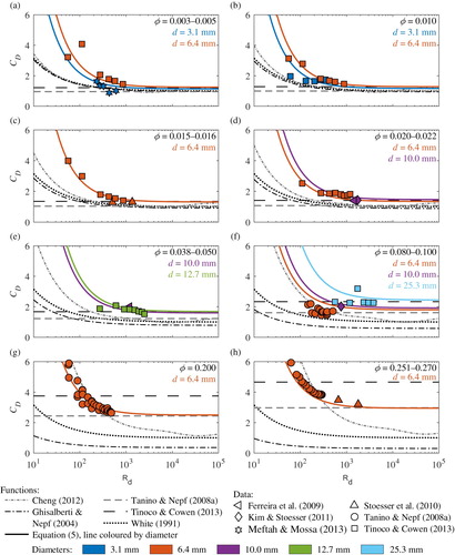
As φ increases, in Fig. e–h, the differences between the
values estimated by each function become greater. The White (Citation1991) and Ghisalberti and Nepf (Citation2004) functions consistently underestimate
. The Ghisalberti and Nepf (Citation2004) function predicts decreasing
with increasing φ, which is unique among the functions presented here. The Cheng (Citation2012) function, in contrast, fits the data reasonably well at higher φ.
The differences between the Tanino and Nepf (Citation2008a) and Tinoco and Cowen (Citation2013) functions become more apparent at higher φ, with the latter estimating greater values of
. Compared to the experimental results, the Tinoco and Cowen (Citation2013) function performs better at lower values of
(Fig. g) while the Tanino and Nepf (Citation2008a) function performs better at higher values (Fig. h). Despite their suggestion otherwise, the Tinoco and Cowen (Citation2013) function performs well at
. The estimates of
made with Eq. (Equation5
(5)
(5) ) fit the data well at higher values of φ.
There are several instances where experimental configurations from the studies in Table overlap such that measurements of were taken at the same φ but at different d. Figure a, b, and f show that across multiple
,
increases with d. Equation (Equation5
(5)
(5) ) reproduces this trend, justifying the dependence of Eq. (Equation5
(5)
(5) ) on d. It is the only function that consistently fits the experimental data in Fig. .
Figure provides a direct comparison between measured and estimated for each function. The Ghisalberti and Nepf (Citation2004) and White (Citation1991) functions (Fig. b and e) consistently underestimate
with RMSE values of 3.09 and 2.40. The Tanino and Nepf (Citation2008a) function (Fig. c) performs better with an RMSE value of 1.66. The Tinoco and Cowen (Citation2013) function (Fig. d) appears to perform well with an RMSE value of 1.16, but shows significant scatter. Horizontal bands in Fig. c and d indicate that the same
value is estimated at the same φ despite different values of d and
. The Cheng (Citation2012) function (Fig. a) also appears to estimate
reasonably well, with an RMSE value of 1.28 as it performs less well at higher
and φ.
Figure 3. Measured compared with estimated
using the functions of (a) Cheng (Citation2012), (b) Ghisalberti and Nepf (Citation2004), (c) Tanino and Nepf (Citation2008a), (d) Tinoco and Cowen (Citation2013), (e) White (Citation1991), and (f) Equation (Equation5
(5)
(5) ); – is a line of equality
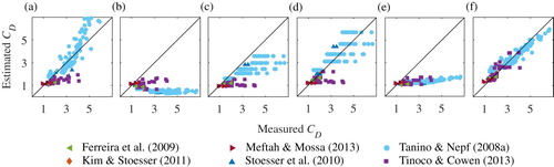
Equation (Equation5(5)
(5) ) (Fig. f) has the tightest clustering around the line of equality with an RMSE value of 0.52, showing that of the six functions evaluated it estimates values of
closest to experimental measurements. Therefore, the dependence of
and
on φ and d suggested by Sonnenwald et al. (Citation2017) is reasonable. Note that these functions have only been tested over the range of
,
, and
and care must be taken applying them outside of this range.
4 Conclusions
A re-parametrization of the Ergun-derived coefficients and
has been presented. This resulted in a function for estimating drag coefficient (
), which has been compared to experimental data alongside several other functions estimating
in arrays of rigid cylinders representing emergent vegetation. All functions perform well for low solid volume fractions (φ) and high cylinder Reynolds number (
), and generally the standard
is not unreasonable here. As
decreases, only those functions that include viscous drag effects provide reasonable results. As φ increases, many of the functions underestimate
. The function detailed in this study, which includes viscous effects, φ, and also a dependency on cylinder diameter (d), provides improved estimates of
.
Notations
| a | = | frontal facing area (m2 m−3) |
| = | drag coefficient (–) | |
| d | = | cylinder diameter (m) |
| g | = | gravity acceleration (m s−2) |
| k | = | turbulent kinetic energy (m2 s−2) |
| = | cylinder Reynolds number (–) | |
| S | = | channel slope (–) |
| s | = | cylinder spacing (m) |
| = | mean interstitial velocity (m s−1) | |
| = | coefficient describing viscous effects (m−1) | |
| = | coefficient describing inertial effects (−) | |
| γ | = | turbulence intensity scaling coefficient (–) |
| ν | = | kinematic viscosity (m2 s−1) |
| ρ | = | density (kg m−3) |
| φ | = | solid volume fraction (–) |
Acknowledgments
The authors thank the anonymous reviewers for their feedback.
ORCID
Fred Sonnenwald http://orcid.org/0000-0002-2822-0406
Virginia Stovin http://orcid.org/0000-0001-9444-5251
Ian Guymer http://orcid.org/0000-0002-1425-5093
Additional information
Funding
References
- Bennett, S. J., Pirim, T., & Barkdoll, B. D. (2002). Using simulated emergent vegetation to alter stream flow direction within a straight experimental channel. Geomorphology, 44(1), 115–126. doi: 10.1016/S0169-555X(01)00148-9
- Cheng, N. S. (2012). Calculation of drag coefficient for arrays of emergent circular cylinders with pseudofluid model. Journal of Hydraulic Engineering, 139(6), 602–611. doi: 10.1061/(ASCE)HY.1943-7900.0000722
- Darby, S. E. (1999). Effect of riparian vegetation on flow resistance and flood potential. Journal of Hydraulic Engineering, 125(5), 443–454. doi: 10.1061/(ASCE)0733-9429(1999)125:5(443)
- Dittrich, A., Aberle, J., Schoneboom, T., Rodi, W., & Uhlmann, M. (2012). Drag forces and flow resistance of flexible riparian vegetation. In W. Rodi & M. Uhlmann (Eds.), Environmental fluid mechanics: Memorial colloquium on environmental fluid mechanics in honour of Professor Gerhard H. Jirka (pp. 195–215). London: CRC Press, Taylor & Francis Group.
- Ergun, S. (1952). Fluid flow through packed columns. Chemical Engineering Progress, 48, 89–94.
- Ferreira, R. M. L., Ricardo, A. M., & Franca, M. J. (2009). Discussion of “Laboratory investigation of mean drag in a random array of rigid, emergent cylinders” by Yukie Tanino and Heidi M. Nepf. Journal of Hydraulic Engineering, 135(8), 690–693. doi: 10.1061/(ASCE)HY.1943-7900.0000021
- Ghisalberti, M., & Nepf, H. M. (2004). The limited growth of vegetated shear layers. Water Resources Research, 40(7), W07502. doi: 10.1029/2003WR002776
- James, C. S., Goldbeck, U. K., Patini, A., & Jordanova, A. A. (2008). Influence of foliage on flow resistance of emergent vegetation. Journal of Hydraulic Research, 46(4), 536–542. doi: 10.3826/jhr.2008.3177
- Kim, S. J., & Stoesser, T. (2011). Closure modeling and direct simulation of vegetation drag in flow through emergent vegetation. Water Resources Research, 47(10), W10511. doi: 10.1029/2011WR010561
- Koch, D. L., & Ladd, A. J. C. (1997). Moderate Reynolds number flows through periodic and random arrays of aligned cylinders. Journal of Fluid Mechanics, 349, 31–66. doi: 10.1017/S002211209700671X
- Marjoribanks, T., Hardy, R., Lane, S., & Parsons, D. (2014). Dynamic drag modeling of submerged aquatic vegetation canopy flows. In A. J. Schleiss, G. de Ceseare, M. J. Franca, & M. Pfister (Eds.), River Flow 2014 (pp. 517–524). London: CRC Press, Taylor & Francis Group.
- Meftah, M. B., & Mossa, M. (2013). Prediction of channel flow characteristics through square arrays of emergent cylinders. Physics of Fluids, 25(4), 045102.
- Nepf, H. M. (1999). Drag, turbulence, and diffusion in flow through emergent vegetation. Water Resources Research, 35(2), 479–489. doi: 10.1029/1998WR900069
- O'Hare, M. T. (2015). Aquatic vegetation–a primer for hydrodynamic specialists. Journal of Hydraulic Research, 53(6), 687–698. doi: 10.1080/00221686.2015.1090493
- Rahman, M. M., Karim, M. M., & Alim, M. A. (2007). Numerical investigation of unsteady flow past a circular cylinder using 2-D finite volume method. Journal of Naval Architecture and Marine Engineering, 4(1), 27–42.
- Rameshwaran, P., & Shiono, K. (2007). Quasi two-dimensional model for straight overbank flows through emergent vegetation on floodplains. Journal of Hydraulic Research, 45(3), 302–315. doi: 10.1080/00221686.2007.9521765
- Rowiński, P. M., & Kubrak, J. (2002). A mixing-length model for predicting vertical velocity distribution in flows through emergent vegetation. Hydrological Sciences Journal, 47(6), 893–904. doi: 10.1080/02626660209492998
- Schlichting, H., Gersten, K., Krause, E., Oertel, H., & Mayes, K.. (1960). Boundary-layer theory (Vol. 7). Berlin: Springer.
- Serra, T., Fernando, H. J. S., & Rodríguez, R. V. (2004). Effects of emergent vegetation on lateral diffusion in wetlands. Water Research, 38(1), 139–147. doi: 10.1016/j.watres.2003.09.009
- Sonnenwald, F., Guymer, I., & Stovin, V. (2017). Computational fluid dynamics modelling of residence times in vegetated stormwater ponds. Proceedings of the Institution of Civil Engineers - Water Management, 171(2), 76–86.
- Sonnenwald, F., Hart, J. R., West, P., Stovin, V. R., & Guymer, I. (2017). Transverse and longitudinal mixing in real emergent vegetation at low velocities. Water Resources Research, 53(1), 961–978. doi: 10.1002/2016WR019937
- Stoesser, T., Kim, S. J., & Diplas, P. (2010). Turbulent flow through idealized emergent vegetation. Journal of Hydraulic Engineering, 136(12), 1003–1017. doi: 10.1061/(ASCE)HY.1943-7900.0000153
- Stone, B. M., & Shen, H. T. (2002). Hydraulic resistance of flow in channels with cylindrical roughness. Journal of hydraulic engineering, 128(5), 500–506. doi: 10.1061/(ASCE)0733-9429(2002)128:5(500)
- Tanino, Y. (2012). Flow and mass transport in vegetated surface waters. In C. Gualtieri & D. T. Mihailovic (Eds.), Fluid mechanics of environmental interfaces (2nd ed., pp. 369–394). Abingdon: Taylor & Francis.
- Tanino, Y., & Nepf, H. M. (2008a). Laboratory investigation of mean drag in a random array of rigid, emergent cylinders. Journal of Hydraulic Engineering, 134(1), 34–41. doi: 10.1061/(ASCE)0733-9429(2008)134:1(34)
- Tanino, Y., & Nepf, H. M. (2008b). Lateral dispersion in random cylinder arrays at high Reynolds number. Journal of Fluid Mechanics, 600, 339–371. doi: 10.1017/S0022112008000505
- Tinoco, R. O., & Cowen, E. A. (2013). The direct and indirect measurement of boundary stress and drag on individual and complex arrays of elements. Experiments in Fluids, 54(4), 1–16. doi: 10.1007/s00348-013-1509-3
- White, F. M. (1991). Viscous fluid flow. New York: McGraw-Hill.