Modelling transverse solute mixing across a vegetation generated shear layer

ABSTRACT

Transverse solute mixing across a vegetation generated horizontal shear layer was quantified using laser induced fluorometry techniques for artificial and real vegetation. A two-dimensional finite difference model (FDM) was developed to describe transverse concentration profiles for flows containing transverse variations in velocity and transverse dispersion, from a steady solute input. The FDM was employed inversely, to optimize the parameters describing the transverse distribution of the transverse dispersion coefficient for vegetation generated shear layers. When laboratory data are available, continuous function descriptions produce slightly improved FDM modelled solute concentration profiles compared with simplified step discontinuity velocity and dispersion inputs. When laboratory data are not available, estimates of step or continuous transverse distributions from other work enable concentration profiles to be predicted with a similar goodness of fit. This paper presents a validated, simple, robust finite difference model to describe the mixing of solutes in a channel containing marginal vegetation.

Keywords:

• Dispersion
• finite difference model
• mixing
• shear effects
• vegetation

1 Introduction

Linear wetlands are increasingly used to provide pollution treatment from diffuse sources such as highways, agricultural land and urban environments. As well as enhancing ecological habitat, wetlands perform a number of services making them suitable for sustainable drainage applications. The reduction in the mean flow velocity promotes sedimentation, whilst a reduction in contaminant concentration can be achieved through dispersion and bio-chemical degradation. It follows that the detention of contamination, and subsequent bio-chemical degradation, is affected by the reach hydrodynamics (Maji et al., 2020; Persson et al., 1999; Koskiaho, 2003).

Vegetation may enhance pollution treatment by increasing the active surface area populated by micro-organisms and, potentially, by promoting dispersion – increasing the likelihood of chemical decay due to sunlight and bio-chemical degradation (Rowinski et al., 2018). Free-surface wetlands, and some rivers, often contain marginal vegetation, creating horizontal shear layers, which lead to complex mixing conditions. Understanding and modelling the spatial variation of mixing due to vegetation generated horizontal shear layers is therefore necessary for improving the treatment of pollutants.

2 Literature review

Mixing across vegetation–water interfaces has been modelled as a shear layer by a number of authors. Whilst most of these studies have focused on the horizontal interface created by submerged vegetation, creating a vertical shear layer, similar processes occur around the vertical interface that occurs between emergent vegetation and open water, creating a horizontal shear layer. Ghisalberti and Nepf (2005) studied the vertical shear layer created by submerged vegetation, whilst White and Nepf (2007) investigated the horizontal shear layer created by the vertical interface at the edge of a patch of emergent vegetation.

Considering the horizontal shear layer White and Nepf (2008) employed a three-zone model of the system to describe flow in the open channel, the mixing layer and the vegetated zone, where the interface is defined as the location of the drag discontinuity. Incident flow is deflected around the patch and becomes a fully developed flow field at a location downstream of the leading edge. The lateral discontinuity in drag leads to a velocity shear generating coherent shear-layer vortices along the vegetation/open-channel interface. These vortices grow to a fixed size and penetrate a certain distance into the vegetation, both being determined by the vegetation drag and the bed friction coefficient (Caroppi et al., 2019). These vortices dominate mass and momentum transport in the system. The occurrence of vortices generates a non-uniform transverse profile of longitudinal velocity that contains an inflection point in the vicinity of the interface (Patil & Singh, 2011; White & Nepf, 2007).

The spatial average velocity in the vegetated zone is controlled by the vegetation drag coefficient, the frontal area per unit volume of the vegetation and the energy gradient (Kadlec, 1990). Conversely, the spatial average velocity in the open channel zone is controlled by the flow depth and bed friction coefficient. Mixing in the vegetation zone comprises both stem scale turbulence and stem scale mechanical processes (Tanino & Nepf, 2008). Nepf (2012) showed that the transverse mixing coefficient, D_y, scaled with the longitudinal velocity, u, and the stem diameter, d. In the open channel zone, transverse mixing is dominated by depth scale shear processes caused by the bed friction and can be approximated using the bed shear velocity, u*, and flow depth, h, through the empirical relation D_y = 0.134u*h (Rutherford, 1994).

To predict mixing in many environmental flow scenarios, it is often sufficient to simplify the study by taking a two dimensional approach, for example in shallow ponds or wetlands, where the vertical effects may be ignored. In such cases solute transport and mixing can be described by the 2D advection-dispersion equation. Rutherford (1994) provides the analytical solution to this equation for steady transverse mixing in an infinitely wide channel with uniform depth, longitudinal velocity and transverse mixing coefficient, downstream of a point source as: (1) $c\left(x,y\right)=\frac{m}{h\sqrt{4\pi D_{y}xu}}\exp \left[\frac{u{\left(y-y_0\right)}^2}{4D_{y}x}\right]$(1) where c(x,y) is the solute concentration, x is the longitudinal distance from the source, y is the transverse position, y₀ is the transverse source location and m is the solute mass inflow rate of the source. This solution assumes that the transverse boundaries are infinitely far away from the source. For a narrow channel, reflecting boundary conditions can be catered for using the method of images (Rutherford, 1994).

Some success has been achieved in modelling solute transport under homogeneous mixing conditions (e.g. uniformly vegetated flows) using a two-dimensional depth-averaged mass transport routing approach (Sonnenwald et al., 2017). In this, an initial patch of solute is discretized into a number of cells and the solute mass in each cell is independently transported and spread longitudinally and transversely at the same velocity and rate (i.e. undergoes uniform advection and dispersion). The principle of superposition is used to combine the individually evolved cell-based sub-masses to create the final two-dimensional solute concentration profile.

Equation (1) is not directly applicable to mixing across shear-layers. Instead, for cases with a transverse depth discontinuity within the cross-section, Kay (1987) produced an analytical solution for an infinitely wide two-zone channel with the discontinuity, located at y = 0. This channel has a deep flow zone (y > 0, subscript 2) and a shallow flow zone (y < 0, subscript 1). Both zones have spatially uniform depth, velocity and transverse mixing coefficient within them and y_i is the distance of the source into the deeper zone. The solution, again for a steady point source, is: (2a) $\begin{array}{rl}c(x,y)& =\frac{m}{2h\sqrt{\pi u_2{D}_{2}x}}\left[\exp \left(-\frac{u_2{\left(y+y_i\right)}^2}{4D_{2}x}\right)\right.\\ & \left.+\frac{h_2\sqrt{u_2{D}_2}-h_1\sqrt{u_1{D}_1}}{h_2\sqrt{u_2{D}_2}+h_1\sqrt{u_1{D}_1}}\exp \left(-\frac{u_2{\left(y-y_i\right)}^2}{4D_{2}x}\right)\right],\\ & y<0\end{array}$(2a) (2b) $\begin{array}{rl}c(x,y)& =\frac{m}{h\sqrt{\pi u_2{D}_{2}x}}\frac{h_2\sqrt{u_2{D}_2}}{h_2\sqrt{u_2{D}_2}+h_1\sqrt{u_1{D}_1}}\\ & \times \left[\exp \left(-\frac{u_1{\left(y+y_i\sqrt{u_2/u_1}\sqrt{D_1/D_2}\right)}^2}{4D_{1}x}\right)\right],y>0\end{array}$(2b) Several mathematical modelling approaches are available for describing the turbulent transport of solute in partially vegetated flows. The most sophisticated is based on a computational fluid dynamics (CFD) approach (Sonnenwald et al., 2019; Yan et al., 2017). In the simplest terms, this consists of a flow model which provides a computed turbulent velocity field for use in a turbulent mass transport model. Although CFD codes have been routinely used for non-vegetated flows for many years, there remain some obstacles to their successful application to partially vegetated flows. For example, doubts remain over the most appropriate way to represent the roughness effects of vegetation patches (Sonnenwald et al., 2016) and there is considerable uncertainty in the appropriate values of several empirical coefficients for such flows.

Turbulent mixing processes due to vegetated shear layers have received much attention, but laboratory studies have been limited to cases using artificial vegetation, formed by distributions of vertical cylinders, either in a regular or random pattern (Ghisalberti & Nepf, 2005; White & Nepf, 2007). Mixing studies in real vegetation have been predominantly conducted in the field for homogeneous vegetation (Huang et al., 2008; Lightbody et al., 2008; Nepf, 1999). The quantification of mixing in real vegetation-generated shear layers, throughout the annual growth cycle, is lacking. Moreover, the application of theory developed in idealized homogeneous conditions has been poorly evaluated in real, heterogeneous flows for two-dimensional engineering applications.

Considering the limitations of many of the modelling approaches discussed, particularly with regards to their applicability to real vegetation, a simple robust approach to modelling the transport and spread of solutes across a shear-layer, suitable for practical application, is desirable. This paper therefore develops a simple 2D finite difference numerical model that is capable of predicting transverse solute concentration profiles created by vegetation-generated horizontal shear layers. It employs prescribed transverse distributions of both the longitudinal velocity and transverse dispersion coefficient. The model has been validated against analytical solutions and has been employed to estimate parameters used to describe the transverse variation of transverse dispersion from new laboratory studies of regular artificial and real vegetation. The paper concludes by exploring methods for estimating the parameters describing the dispersion coefficient distributions from previously published research.

3 Laboratory study

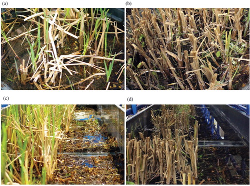
The mixing characteristics of emergent vegetation-generated horizontal shear layers were investigated using laser induced fluorometry (LIF) and acoustic Doppler-shift velocimetry (ADV) in a controlled 24 m long, 1 m wide horizontal laboratory flume at the University of Warwick, UK. Two artificial vegetation stem densities, of 1594 and 398 stems m⁻², with solid volume fractions, φ, of 0.02 and 0.005, respectively, were investigated using a 7.5 m long linear array of emergent 4 mm diameter cylinders with laterally staggered geometry (Fig. 1). The artificial vegetation tests provided an idealized case from which to evaluate the application of the Ghisalberti and Nepf (2005) flux-gradient model (West, 2016). Two natural vegetation cases were also studied by installing winter and summer season Typha latifolia (φ = 0.01 and φ = 0.019 respectively), supplied directly from a cultivator (Salix UK), in the flume (Fig. 2a and b, respectively). The vegetation was within its natural bed and was fixed into the bed of the channel using pre-inserted steel spikes. The first set of experiments considered conditions where for the four vegetation types the vegetation extended over the full width of the channel. The second set of experiments considered a partially vegetated channel: for the artificial vegetation cases, the vegetation had a width of 600 mm (Fig. 1); for the natural vegetation cases, the vegetation was cropped to a width of 500 mm along the channel centreline, such that the bed of the open channel region was the same natural bed (Fig. 2c and d). Vegetation was installed upstream of the injection location for a distance of 1.8 m or 5.0 m for the artificial and real vegetation, respectively. Comprehensive vegetation characteristics are provided in Sonnenwald et al. (2017). Observations from three of the fully vegetated cases are used in final testing of the model, particularly in regard to optimizing its parameters (Section 4). Later in this paper, observations from the partially vegetated cases are used to investigate the transverse variation in transverse dispersion coefficient (Section 5). The complete dataset can be accessed at West et al. (2018) (https://doi.org/10.15131/shef.data.7077386.v1).

Figure 1 Schematic plan view of experimental set-up for artificial partially vegetated case, showing low density (red) and high density (black and red) stem patterns

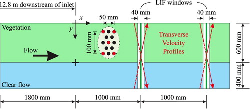
Figure 2 Experimental configurations for winter Typha (a, c) and summer Typha (b, d). (a) and (b) show details of the vegetation, illustrating the different stem densities for (a) winter φ = 0.01 and (b) summer φ = 0.019. (c) and (d) show the how the vegetation was cropped along the channel centreline, revealing the natural bed in the open channel region (right hand side)

A continuous vertical line source of Rhodamine 6G fluorescent tracer was made at the vegetation/clear flow interface. Transverse concentration profiles were measured 1.0 m and 2.0 m downstream of the injection using a 532 nm wavelength laser (Changchun New Industries Optoelectronics Tech. Co. Ltd., Changchun, Jilin Province, P.R. China) (CNI 200 mW, 532 nm DPSS laser, Model: MGL-III-532-200 with PSU-III-FDA power supply) mounted at the flow mid-depth. A CCD camera (FLIR Systems, Wilsonville, Oregon, USA) (Point Grey 1.3MP On Semi VITA CMOS 1/2′′ Monochrome, Global 2) positioned underneath the flume, below a 40 mm wide glass window, recorded images of the laser beam at 5 Hz. The injection rate was adjusted to ensure that the upstream LIF measurements were utilizing the full greyscale range of the cameras. A cut-off filter was installed above the camera to prevent excitation light reaching the camera. The LIF system was calibrated, taking account of the variation in power attenuation, given the heterogeneous distribution of tracer concentration, after Ferrier et al. (1993), as described in Sonnenwald et al. (2017).

The measurement of the transverse variation in the longitudinal velocity was developed throughout this study. In the initial set-up, for the high density artificial vegetation, a Nortek Vectrino II vertical profiler was used, with measurements made at only 16 points, approximately 60 mm spacing, across the 1 m channel width, which prevented the determination of the boundary shear layer. This was improved by employing Metflow Ultrasound Velocity Profiling (UVP) from an array of ultrasound transducers in the walls of the flume at the flow mid-depth. For winter Typha, a single UVP probe was used at both of the upstream and downstream boundaries. However, in this configuration, readings were limited to recording the velocities between 100 and 900 mm from the channel walls. The remaining 100 mm adjacent to each side wall was assumed to be constant, and hence these data do not show the boundary layer at the side walls. In the final set-up, used for low density artificial vegetation and summer Typha, two UVP probes were installed at both upstream and downstream boundaries, one at each side of the channel, each recording the first 750 mm, ensuring that the central 500 mm of the flow had two values recorded. For this configuration, shown in Fig. 1, the boundary shear at the side walls is clearly visible in the results. Velocity data were filtered using the phase-space filtering technique developed by Goring and Nikora (2002) and a mean velocity profile was calculated from the average of the upstream and downstream locations. Further details can be found in West (2016).

A constant flow depth of 0.15 m was selected, measured to 0.1 mm accuracy using a Vernier gauge and controlled with the use of a downstream tailgate at the channel outlet. Five discharges were investigated (3.35, 4.25, 5.25, 6.35 and 7.35 l s⁻¹) such that in-vegetation velocity was representative of velocities found in real vegetation (e.g. Huang et al., 2008; Koskiaho, 2003; Lightbody et al., 2008; Nepf, 1999).

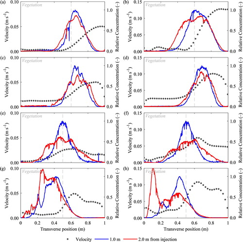
Figure 3 presents measurements, for both artificial and real heterogeneous vegetation cases, of the mean transverse velocity profile (filled circles) and the transverse tracer concentration profiles, recorded at the LIF sections 1.0 m (blue line) and 2.0 m (red line) downstream from the injection, at the highest and lowest discharges studied. Both the velocity and tracer concentration data recorded for real vegetation exhibit greater variations throughout the cross-section compared with the artificial vegetation caused by the heterogeneous nature of the material, as shown in Fig. 2.

Figure 3 Transverse velocity and concentration profiles at Q = 3.4 × 10⁻³ m³ s⁻¹ (left) and Q = 7.5 × 10⁻³ m³ s⁻¹ (right) for (a, b) low-density artificial vegetation; (c, d) high-density artificial vegetation; (e, f) winter Typha; and (g, h) summer Typha

4 Modelling framework

This section describes the development of a 2D finite difference numerical model that can be used to predict transverse solute concentration profiles given arbitrary transverse velocity and transverse mixing coefficient distributions. After validation, the model was employed inversely, to optimize the parameters within a pre-defined function developed to describe the transverse variation of transverse dispersion coefficient.

Model selection

For the present study, the velocity field was available from observations, so no flow model was required, but the heterogeneous mixing conditions were not appropriate for the routing approach mentioned above. Additionally, for steady line sources the mass transport problem can be reduced to one having a less sophisticated two-dimensional mathematical description than that required for unsteady sources. It was also anticipated that the study’s objective of optimizing a mathematical model in order to identify the distribution of a mixing coefficient would be more tractable when using a simplified approach.

Since the effect of longitudinal mixing is negligible for steady sources (Rutherford, 1994) the transverse and longitudinal evolution of a steady vertical line source in a straight, uniform channel is governed by the interaction of longitudinal advection and transverse mixing. This is described by: (3) $h\left(y\right)u\left(y\right)\frac{\mathrm{\partial }c\left(x,y\right)}{\mathrm{\partial }x}=\frac{\mathrm{\partial }}{\mathrm{\partial }y}\left[h\left(y\right)D_y\left(y\right)\frac{\mathrm{\partial }c(x,y)}{\mathrm{\partial }y}\right]$(3) where h(y), u(y) and D_y(y) are transverse distributions of the depth, longitudinal velocity and transverse mixing coefficient, respectively. Note that this equation allows for transverse variations in depth, longitudinal velocity and transverse mixing coefficient, but all of these are constant in the longitudinal direction. At both banks of the channel the transverse solute flux is zero (i.e. reflecting conditions), so that the boundary conditions are described, at both banks, by: (4) $D_y\left(y\right)\frac{\mathrm{\partial }c(x,y)}{\mathrm{\partial }y}=0$(4) Although exact analytical solutions to the system described by Eqs (3) and (4) are available for a very small number of special cases, in order to apply the equations to identify an otherwise unknown distribution of transverse mixing coefficient, some form of approximate numerical solution of them is required. The following section describes the formulation of the model from the point of view of undertaking a simulation.

Model development

A numerical solution was sought to overcome the limitations of the flux gradient model outlined by Ghisalberti and Nepf (2005). There are many finite difference and finite volume schemes available to solve advective-transport problems (Abbott & Basco, 1989; Versteeg & Malalasekera, 2007). In sympathy with the simple approach adopted for this study, a robust but low-order finite difference scheme was used. The main advantages of this approach were that the likely sources of, and the nature of, any numerical errors were well known and solutions could be developed easily. The main disadvantage of this approach was that a significant amount of model testing was required to ensure that sufficiently refined discretizations, to eliminate significant numerical errors, were used in the two-dimensional spatial plane involved. The solution method for Eq. (3) and its boundary conditions is described in Appendix 1.

Model validation

To investigate the sensitivity of solutions to numerical errors caused by the spatial discretization, the two analytical solutions from Rutherford (1994) and Kay (1987) (Eqs 1 and 2) were used to test the numerical model. An attempt was also made to modify Kay’s analytical solution for application to a finite-width channel, by imposing no-flux transverse boundary conditions. This was undertaken by “reflecting” solute back into the channel using the method of images. This was successful until the “reflected” solute encountered the step-change in velocity and mixing conditions: when this occurred, the solution broke down. Further work on this is needed before its potential can be exploited fully, but it was used in sensitivity testing to mitigate the impact of the narrow channel on the accuracy of the Kay solution compared to the FDM model, which does have appropriately represented reflecting boundaries.

The testing philosophy was to investigate the numerical solution for channel geometries, and over ranges of parameters, that were relevant to the experimental conditions for which the model was to be applied later. So a uniform depth (transversely and longitudinally) channel 6 m long, 1 m wide, with longitudinal velocities between 0.005 and 0.2 m s⁻¹ and transverse mixing coefficients between 10⁻⁵ and 10⁻³ m² s⁻¹ was used. For Eq. (1) the velocity and mixing coefficient were constant over the width of the channel, whereas for Eq. (2), smaller parameter values were specified in one half of the width (vegetated, slow zone) than in the other half (clear flow, fast zone), e.g. a velocity of 0.02 m s⁻¹ with a mixing coefficient of 10⁻⁴ m² s⁻¹ in the slow zone and a velocity of 0.2 m s⁻¹ with a mixing coefficient of 10⁻³ m² s⁻¹ in the fast zone. Various steady source locations were employed. For each combination of parameter values solutions were obtained for successive reductions in longitudinal and transverse discretization steps. The results of the model testing are briefly summarized in the following paragraphs.

It was found that converged numerical solutions would be obtained for Rutherford’s case provided that Δx ≤ 0.05 m and Δy ≤ 0.01 m and for Kay’s case provided that Δx ≤ 0.01 m and Δy ≤ 0.005 m. In other words, further refinements in the spatial discretization yielded no change in the simulated concentration field. The above values reflect the presence of smaller concentration gradients in the longitudinal direction compared to the transverse direction and the more complex transverse flow structure of Kay’s case. Example comparisons between the numerical and the analytical solutions are provided in non-dimensional form in Fig. 4. In all cases the analytical solutions were computed independently by the authors rather than relying on the figures in the published sources, and the numerical solutions were obtained using the upper discretization limits given above. For reasons of clarity the results from both cases are shown in a common non-dimensional manner, so that, at first sight, the analytical solution plots may appear to be different to those shown in the original sources. In Fig. 4b, the velocity and mixing coefficient distributions are summarized to the left of the plot.

Figure 4 Comparison of model results (symbols) with analytical solutions (lines) for non-dimensional concentration, c*, where c* = c/c_s1 and c_s1 is the total mass flux at location x* = 1. (a) Rutherford (1994) – uniform conditions – source at y* = 0.25 for U = 0.1 m s⁻¹; D_y = 1 × 10⁻² m² s⁻¹, where w is channel width and (b) Kay (1987) – step variation – source at y* = 1.0 for flow rate 2 × 10⁻³ m³ s⁻¹; u₁ = 0.1 m s⁻¹; D₁ = 1 × 10⁻² m² s⁻¹; with depth in y* > 0 twice that in y* < 0

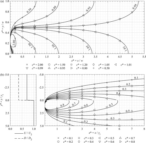
Figure 4a compares the numerical solution for the transversely uniform conditions with the analytical solution shown in fig. 3.7a of Rutherford (1994). Clearly, there is very good agreement. Figure 4b compares the numerical solution for the transverse discontinuity case with the analytical solution shown in fig. 5c of Kay (1987). Although the corresponding convergence tests were undertaken for a narrow channel of uniform depth (reflecting the laboratory conditions described in Section 3), the numerical solutions in Fig. 4b were obtained for a wide channel with a transverse step-change in depth in order to be directly comparable with the analytical solution. Again, there is very good agreement. Overall the results were shown to be independent of grid scale and the model successfully reproduced the two dimensional concentration distributions compared to analytical solutions.

Model application

In contrast to the simulation tests against analytical solutions described above, the numerical model was also tested by applying it to several cases of observed solute transport in uniformly vegetated conditions as described in Section 3 and presented in more detail in Sonnenwald et al. (2017). These applications mimicked the sort of modelling described in Section 5 and provided further confidence that, not only was the numerical model reliable, but the optimization method was successful.

The aim of these tests was to identify the optimum homogeneous transverse mixing coefficient, given observed transverse concentration profiles at two longitudinal locations for a steady vertical line source using an available estimate of the homogeneous longitudinal velocity. Using the upstream transverse concentration profile as the upstream boundary condition, optimization of the mixing coefficient was achieved by repeating simulations for various coefficient values and identifying the simulation having the best fit to the corresponding downstream transverse concentration profile. In these model runs the discretization parameters were: Δx = 0.01 m and Δy = 0.005 m. Data for three vegetation types (continuous injection tracer studies were not performed for the low-density artificial vegetation) and five flow rates were used. Optimized mixing coefficients were compared with those obtained using the twodimensional routing procedure introduced in Section 2 (Sonnenwald et al., 2017) modified to account for a continuous injection.

The mean and standard deviation (over the 15 cases considered) of the difference between the mixing coefficients obtained from the numerical model and the routing procedure were 5.4 × 10⁻⁶ and 1.2 × 10⁻⁵ m² s⁻¹, respectively. In general, these differences were two orders of magnitude smaller than the mixing coefficient being estimated, suggesting good agreement between the two approaches. The relatively large value for the standard deviation was caused by the significant heterogeneity of the summer Typha.

For application to the problem of horizontal vegetated shear layers, adapting the approach of Ghisalberti and Nepf (2005) who studied a vertical shear layer caused by submerged vegetation, a continuous distribution was assumed for the transverse variation of the transverse dispersion coefficient (Fig. 5). The peak transverse dispersion coefficient, D_P, was assumed to occur at the vegetation–clear flow interface, with fixed, constant values of D₁ and D₂ at large distances away from the interface, in the vegetation and the clear flow, respectively. Either side of the peak, semi-Gaussian profiles were assumed, which provide smooth continuous transitions, with the spread away from the peak independently defined by the standard deviations σ₁ and σ₂. The optimization problem was therefore formulated as maximizing the goodness of fit $R_t^2$ (Young et al., 1980) between simulated and observed concentration profiles within the limits of 1 × 10⁻⁸ m² s⁻¹ and 0.1 m² s⁻¹ for the transverse dispersion coefficients and 1/3w and 3Δy for the standard deviations, where w is channel width and Δy is the transverse discretization step size. This was implemented with the MATLAB function fmincon by taking the negative of the $R_t^2$.

Figure 5 Assumed continuous dispersion coefficient distribution, illustrating values for D₁, D₂, D_P, σ₁ and σ₂, where y* = y/y₀, y₀ indicates the location of the interface and y* < 1 is within vegetation

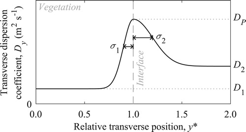
The constraints assume that transverse dispersion at the interface is greater than transverse dispersion within both the vegetation (D_p > D₁) and the open water (D_p > D₂). The minimum value of transverse dispersion coefficient was chosen to be slightly greater than molecular diffusion, whilst the maximum value was chosen to be larger than any values of transverse dispersion in vegetation reported by Sonnenwald et al. (2017). The lower and upper limits of the spread were chosen to ensure that the continuous dispersion coefficient profile could not collapse to almost a step profile by being too small or expand to more than 2/3 of the channel width.

5 Results

Having obtained laboratory measurements of velocity and tracer spread due to a vegetation generated shear layer, this section compares the ability of two different transverse parameter distribution types to predict the observed transverse concentration profiles. Following this, using previously published relationships, an approach to estimate one of the dispersion parameter distribution types is explored.

Parameter identification

The numerical model developed above was used to compare a transverse step distribution (i.e. a discontinuity) with a continuous transverse distribution, for both longitudinal velocity and transverse dispersion, to simulate transverse solute concentration profiles. For the step distribution, width mean velocities within the vegetated and unvegetated zones were obtained by averaging the recorded experimental velocity distributions either side of the interface between the two zones. For the continuous parameter distribution, the recorded experimental velocities were used. The model was run to obtain optimized values of the parameters to describe the transverse dispersion distribution: two for the step distribution (D₁ and D₂) and five for the continuous distribution (D₁, D₂, D_P, σ₁ and σ₂). The model used the observed transverse tracer concentration profile at 1 m downstream from the injection site (upstream boundary condition) as input to optimize the prediction of the corresponding tracer concentration profile at 2 m downstream of the injection site. As above, the discretization parameters were Δx = 0.01 m and Δy = 0.005 m. Fully reflecting transverse boundary conditions were used. The resulting spatial distributions of the transverse dispersion coefficient and the predicted concentration profiles are compared for the lowest and highest flow rate cases for artificial and real vegetation in Figs 6 and 7, respectively. Note that the dispersion coefficients have been non-dimensionalized with the transverse mean flow velocity (across the full width of the channel) and with the stem diameter. Table 1 summarizes the goodness of fit of the optimized predicted concentration profile to the observed profile for all cases.

Figure 6 Comparison between optimized step (S) and continuous (C) distributions of dispersion coefficient (left) and predicted concentration profiles (right) for (a–d) low-density artificial vegetation, and (e–h) high-density artificial vegetation, where (a), (b), (e), and (f) are for Q = 3.4 × 10⁻³ m³ s⁻¹ and (c), (d), (g), and (h) are for Q = 7.5 × 10⁻³ m³ s⁻¹

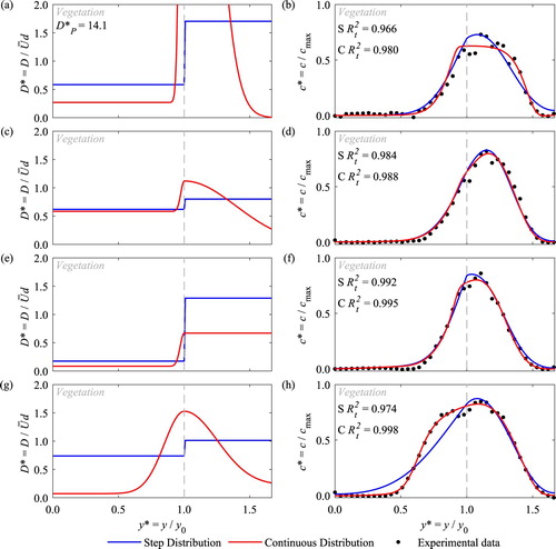
Figure 7 Comparison between optimized step (S) and continuous (C) distributions of dispersion coefficient (left) and predicted concentration profiles (right) for (a–d) Winter Typha, and (e–h) Summer Typha, where (a), (b), (e), and (f) are for Q = 3.4 × 10⁻³ m³ s⁻¹ and (c), (d), (g), and (h) are for Q = 7.5 × 10⁻³ m³ s⁻¹

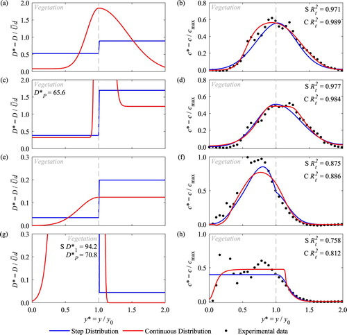
Table 1 Summary of goodness of fit, $R_t^2$, values between laboratory data and predicted spatial concentration profiles for step, continuous and estimated dispersion distributions

		Transverse velocity and dispersion parameter distributions
		Optimized		Estimated
Vegetation type	Discharge Q (10^−3 m^3 s^−1)	Step	Continuous	Step	Continuous
Low-density AV	3.4	0.966	0.980	0.921	0.950
	4.2	0.951	0.978	0.888	0.918
	5.2	0.975	0.981	0.948	0.973
	6.4	0.974	0.980	0.954	0.978
	7.5	0.984	0.988	0.963	0.986
	Mean	0.970	0.981	0.935	0.961
High-density AV	3.4	0.992	0.995	0.960	0.962
	4.2	0.987	0.975	0.956	0.955
	5.2	0.947	0.996	0.835	0.835
	6.4	0.989	0.998	0.922	0.923
	7.5	0.974	0.998	0.909	0.908
	Mean	0.978	0.992	0.917	0.917
Winter Typha	3.4	0.971	0.990	0.778	0.774
	4.2	0.981	0.990	0.784	0.795
	5.2	0.980	0.988	0.745	0.786
	6.4	0.983	0.990	0.745	0.798
	7.5	0.977	0.984	0.729	0.754
	Mean	0.978	0.988	0.756	0.781
Summer Typha	3.4	0.875	0.886	0.867	0.866
	4.2	0.696	0.764	0.674	0.674
	5.2	0.793	0.863	0.729	0.728
	6.4	0.728	0.784	0.434	0.425
	7.5	0.758	0.812	0.491	0.486
	Mean	0.770	0.822	0.639	0.636
Mean		0.924	0.946	0.812	0.824

AV = artificial vegetation.

For three of the four vegetation conditions studied, both the step and continuous velocity and dispersion distributions are able to predict concentration profiles in close agreement with the measured data and have similar values of $R_t^2$. The exception is summer Typha (Figs 7f and h), where the continuous velocity and dispersion coefficient distributions perform noticeably better, with mean $R_t^2$ of 0.822 compared to 0.770 (Table 1). The good performance of the continuous dispersion distributions has confirmed the semi-Gaussian trend around the interface. At the lowest discharge, the high density artificial vegetation (Fig. 6e) and the summer Typha (Fig. 7e) cases do not show noticeable non-dimensional peak dispersion values. This is in contrast to the very high non-dimensional peak dispersion parameters of 14.1, 65.5 and 70.8, shown in Figs 6a, 7c and g, respectively, where close to the vegetation interface, around which the transverse concentration profile shows little transverse gradient, the optimum is poorly defined. This is a similar restriction to that which affects the gradient flux approach of Ghisalberti and Nepf (2005), alluded to in Section 2 (West, 2016).

Table 1 provides the goodness of fit, $R_t^2$, values between the observed and predicted transverse concentration profiles for the step and continuous parameter distributions for all the vegetated conditions and discharges studied. The values show that, in almost all the cases (19 out of 20), the continuous velocity and dispersion distributions predict tracer concentration profiles closer to the observations than those predicted by the step velocity and dispersion distributions. For all the summer Typha discharge cases, the quality of both the step and continuous parameter distribution predictions is poorer than the rest of the cases, illustrating the difficulty of predicting dispersion in real vegetation. Considering the other three vegetation conditions, in the majority of cases the high density, artificial vegetation is simulated better than the other two vegetation conditions, as reflected in the mean $R_t^2$ values shown in Table 1.

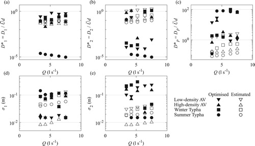
Looking for any general trends in the parameters, Fig. 8 (filled symbols) presents the optimized continuous dispersion coefficient distribution parameters, as a function of flow rate. In general, the dispersion parameter values, optimized from fitting to the measured concentration profiles, are within the following ranges: $D_1^{\ast }$ 0.01 to 1; $D_2^{\ast }$ 0.0001 to 1; $D_p^{\ast }$ 1 to 100; with σ₁ and σ₂ 0.015 to 0.1 m and 0.03 to 0.25 m, respectively. There is a large range of values and much scatter in these optimized parameters. In addition, the high density real vegetation, i.e. the summer Typha, appears to be significantly different to the other experimental conditions (e.g. Fig. 8a), whilst the low density real vegetation, i.e. winter Typha, exhibits four orders of magnitude difference between low and high discharges for $D_2^{\ast }$ (Fig. 8b), with two orders of magnitude difference across several of the other parameters. $D_2^{\ast }$ would be expected to increase with discharge due to increasing bed-shear, but this is not reliably shown for any vegetation type. Such variations might be expected from experiments using real vegetation, so it may be more revealing to focus on the artificial vegetation cases.

Figure 8 Comparison between optimized (filled) and estimated (open) continuous transverse dispersion coefficient distribution parameters with respect to flow rate

For the artificial vegetation cases, considering variations with discharge: $D_1^{\ast }$ is approximately constant for both vegetation densities, whilst $D_2^{\ast }$, $D_P^{\ast }$ and σ₁ show too much scatter to discern any trends. On the other hand, σ₁ shows a weak increase with discharge for both vegetation densities. Considering the effects of vegetation density: the magnitude of both $D_1^{\ast }$ and σ₂ decreases from low density artificial to high density artificial, i.e. in accordance with volume fraction, whilst $D_2^{\ast }$ and σ₁ show the opposite trend. There appears to be no discernible trend in the variations of $D_P^{\ast }$ with vegetation density.

5.2 Parameter estimation

Having shown that continuous velocity and transverse dispersion coefficient distributions are slightly better than step distributions for predicting solute mixing around the vegetation generated shear layer, this section explores how we can independently obtain estimates of the distributions from previously published research. For the step distributions this only requires two velocity and two dispersion coefficients, whilst the continuous transverse distributions of longitudinal velocity and transverse dispersion require many more parameter values.

White and Nepf (2008) provide a method for calculating the transverse variation in longitudinal velocity across a vegetation generated shear layer. Following this approach, the velocities in the vegetated and clear water zones, i.e. u₁ and u₂, respectively, and hence ΔU (= u₂ – u₁), have been taken from the observed velocity field. No further estimation is required for the step velocity distribution, whilst for the continuous velocity distribution, only the transition between these two values has been estimated. The drag coefficient, C_D, and bed friction coefficient, C_f, have been estimated from Sonnenwald, Stovin, et al. (2019) and Rameshwaran and Shiono (2007), respectively. A roughness factor k_s = 0.16 mm and channel slope S = 1/10,000 have been assumed. Using these, a continuous transverse velocity distribution can be estimated, examples of which are shown in Fig. 9 (left column). D₁ has been estimated from Tanino and Nepf (2008), with D₂ being estimated from eq. (37) in White and Nepf (2008), and D_P being based on fig. 15 in White and Nepf (2008), where the 0.7 scaling parameter is modified to 1.0. σ₁ and σ₂ were taken as δI and δO, respectively, using eqs (39) and (40) in White and Nepf (2008). The estimated continuous transverse dispersion distributions are also shown in Fig. 9 (left column).

Figure 9 Estimated continuous velocity and transverse dispersion distributions (left), with resulting concentration profile compared with laboratory measurements (right), for (a, b) low-density artificial vegetation, and (c, d) high-density artificial vegetation, at Q = 7.5 × 10⁻³ m³ s⁻¹ and for (e, f) winter Typha, and (g, h) summer Typha, at Q = 3.4 × 10⁻³ m³ s⁻¹

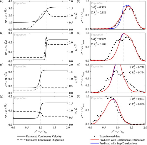
The estimated continuous transverse dispersion coefficient distribution parameters are shown in Fig. 8 (open symbols), where values are within the following ranges: $D_1^{\ast }$ 0.03 to 0.1; $D_2^{\ast }$ 0.05 to 1.0; $D_P^{\ast }$ 0.1 to 2.0; with σ₁ and σ₂ 0.01 to 0.1 m and 0.01 to 0.05 m, respectively. $D_1^{\ast }$ appears approximately constant with discharge and vegetation type, and shows little scatter, whilst the other four parameters all exhibit a weak increase with respect to discharge across all the vegetation types. $D_2^{\ast }$ and $D_P^{\ast }$ decrease with increasing volume fraction (low density artificial, low density real, high density artificial, high density real), with similar variations for both spread parameters, σ₁ and σ₂. Comparing these estimated parameter values with the corresponding ones obtained by optimizing the numerical model to the observed data (Fig. 8) indicates limited agreement. Whereas differences may be up to one order of magnitude for $D_1^{\ast }$, σ₁ and σ₂, differences for the other two parameters are typically much larger. $D_1^{\ast }$ is underestimated, and the larger optimized $D_1^{\ast }$ is consistent with the findings of Sonnenwald et al. (2017). The larger optimized values of σ₂ suggest a greater influence of the shear-layer on the open-channel than predicted by White and Nepf (2008), which may be a limitation of the eddy-viscosity based approach.

A comparison between observed concentration profiles and those predicted with the numerical model using the estimated step and continuous velocity and transverse dispersion coefficient distributions is provided in Fig. 9. Overall, these results suggest that using estimated parameters to predict concentration profiles, for either step or continuous functions, across a vegetation generated shear layer can give good results for the artificial vegetation, with $R_t^2$ around 0.9 (Table 1). This predictive capability decreases in real vegetation: the winter Typha has a mean $R_t^2$ value of approximately 0.76, whilst in the most heterogeneous vegetation case, the summer Typha, the mean $R_t^2$ falls to 0.64, with a significant difference between high and low flow rates. In some cases, the peak concentration at the interface is overestimated, with slight underestimations in the spread, but there is little difference between the concentration profiles from step and continuous parameter distributions.

6 Discussion

Table 1 provides the goodness of fit, $R_t^2$, between concentration profiles predicted using optimized step and continuous distributions of velocity and dispersion coefficient and using corresponding distributions estimated from previously published studies. In all the cases studied, the concentration profiles obtained with the optimized parameters are better than those obtained with the estimated parameters.

To parameterize the transverse distribution of dispersion coefficients, the inverse modelling approach is limited when there are no, or very low, transverse concentration gradients, which is also the limitation of the gradient flux approach. Uncertainty and noise in the solute concentration measurements reported may be caused by a combination of the trapping of tracer in the 40 mm wide vegetation-free viewing windows and, in the Typha studies, the heterogeneity of the vegetation. Despite these limitations, the numerical modelling approach described has been shown able to characterize the spread of a tracer across a vegetation generated shear layer using either a step or continuous distribution. The results presented in Fig. 8 show variations with respect to discharge and they confirm that the seasonal variation is greater than the variation with discharge. This warrants further investigation, as the quantification of mixing in real vegetation generated shear layers throughout the annual growth cycle in the literature is limited.

Whilst the results presented here compare step with continuous distributions, these comparisons have been performed by changing two parameters, namely the longitudinal velocity and the transverse dispersion coefficient. In this case, for vegetation generated shear layers, the difference between predicted concentration profiles is so subtle that further analysis of each parameter individually is not warranted. However, there are other contexts, for example between the main channel and the over-bank region in compound channel flows and between onshore and offshore mixing due to waves breaking, where such spatial parameter distributions may have a greater impact. The development of the numerical model also provides a framework for undertaking inverse modelling of mixing data to investigate the spatial distribution of transverse dispersion parameters in other scenarios.

7 Conclusions

A simple, robust two-dimensional finite difference model of steady solute transport has been developed and validated against analytical solutions. It is able to predict transverse solute concentration profiles across vegetation-generated shear layers given transverse distributions of both the longitudinal velocity and the transverse dispersion. The numerical model has been employed inversely to parameterize transverse distributions of transverse dispersion coefficients from new observed solute concentration profiles, at the laboratory scale, for two cases of artificial and real vegetation at several flow rates. There is considerable spread in the parameter values obtained. The ability to estimate the transverse distribution of velocity and transverse dispersion, using previously published relationships, was investigated. Model predictions using both the step and continuous distributions of velocity and transverse dispersion show similar goodness of fit to the observed concentration data. The limited fit, especially for high flow rates under summer Typha, illustrates the need for improved predictive techniques to describe mixing within real vegetation and across natural vegetation generated shear layers.

Notation

c(x,y)	=	solute concentration (kg m−3)
CD	=	drag coefficient (–)
Cf	=	bed friction coefficient (–)
d	=	stem diameter (m)
Dy	=	transverse mixing coefficient (m2 s−1)
h	=	flow depth (m)
i	=	the finite number of longitudinal computational nodes (–)
j	=	the finite number of transverse computational nodes (–)
ks	=	roughness factor (m)
m	=	the solute mass inflow rate of the source (kg s−1)
N	=	number of nodes (–)
p, q and r	=	functions of α, β, γ, δ
$R_t^2$	=	goodness of fit (–)
S	=	channel slope (–)
u	=	longitudinal velocity (m s−1)
u*	=	bed shear velocity (m s−1)
w	=	channel width (m)
x	=	longitudinal distance from the source (m)
y	=	transverse position (m)
yi	=	the distance of the source into the deeper zone (m)
y0	=	transverse source location (m)
y*	=	relative transverse position (–)
σi	=	standard deviations (m)
φ	=	solid volume fractions (–)
Δx	=	longitudinal discretization step size (m)
Δy	=	transverse discretization step size (m)
α, β, γ and δ	=	model coefficients
subscript 1	=	shallow flow zone, y < 0; vegetated zone
subscript 2	=	deep flow zone, y > 0; clear water
subscript p	=	peak value

Acknowledgements

Many thanks go to Mr Ian Baylis who provided the technical support for all the laboratory studies conducted at the University of Warwick.

Supplemental data

Supplemental experimental data can be accessed from West, P., Hart. J., Sonnenwald, F., Stovin, V., and Guymer, I. (2018). Transverse dispersion in vegetation across a shear-layer 2016: Artificial, Carex, Typha [data set] https://doi.org/10.15131/shef.data.7077386.v1

Additional information

Funding

This work was supported by the EPSRC (Grant nos. EP/K025589/1, EP/K024442/1 and EP/P012027/1). P. West was supported by an EPSRC studentship at the University of Warwick, under EP/K503204/1.

Appendix A – Solution Method

The finite difference approximation to Eq. 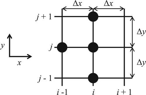(3) took the form: (A1) $\begin{array}{rl}& \frac{h^j{u}^j\left[c_i^j-c_{i-1}^j\right]}{\mathrm{\Delta }x}\\ & =\frac{1}{\mathrm{\Delta }y}\left\{\frac{\left(h^{j+1}{D}^{j+1}+h^j{D}^j\right)}{2}\frac{\left[c_i^{j+1}-c_i^j\right]}{\mathrm{\Delta }y}\right.\\ & \left.-\frac{\left(h^j{D}^j+h^{j-1}{D}^{j-1}\right)}{2}\frac{\left[c_i^j-c_i^{j-1}\right]}{\mathrm{\Delta }y}\right\}\end{array}$(A1) where h, u, D and c are as previously defined, Δx and Δy are the discretization steps in the longitudinal and transverse directions, respectively, and superscripts i and j refer to the finite number of computational nodes at which h, u, D and c have numerical values (i representing longitudinal location and j representing transverse location). Since h, u and D do not vary longitudinally, subscripts are not required. Equation (A1) represents an “upwind” treatment of longitudinal advection and a “central” treatment of transverse mixing for the approximation of Eq. (3) at node i, j. Figure A1 illustrates the “computational molecule” in the computational plane.

After grouping of terms, Eq. (A1) can be written as: (A2) ${\alpha }^{j-1}{c}^{j-1}+{\text{β}}^j{c}^j+{\gamma }^{j+1}{c}^{j+1}={\delta }^j$(A2) where the coefficients α, β, γ and δ are functions of Δx, Δy and nodal values of h, u and D (all of which are known). α, β, γ and δ are given as: (A3) $\begin{array}{rl}{\alpha }^{j-1}& =\frac{-\left(h^{j-1}{D}^{j-1}+h^j{D}^j\right)}{2\mathrm{\Delta }{y}^2}\end{array}$(A3) (A4) $\begin{array}{rl}{\text{β}}^j& =\frac{h^j{u}^j}{\mathrm{\Delta }x}+\frac{(h^{j+1}{D}^{j+1}+2h^j{D}^j+h^{j-1}{D}^{j-1})}{2\mathrm{\Delta }{y}^2}\end{array}$(A4) (A5) $\begin{array}{rl}{\gamma }^{j+1}& =\frac{-\left(h^{j+1}{D}^{j+1}+h^j{D}^j\right)}{2\mathrm{\Delta }{y}^2}\end{array}$(A5) (A6) $\begin{array}{rl}{\delta }^j& =\frac{h^j{u}^j}{\mathrm{\Delta }x}{c}_{i-1}^j\end{array}$(A6)

Assuming there are N nodes in the transverse direction, application of Eq. (A2) to all interior nodes yields N−2 equations containing N unknown values of solute concentration. The remaining two equations required to solve for all nodal values of solute concentration come from applying the boundary conditions at the first and last transverse nodes (see below). The system of equations forms a tri-diagonal matrix and was solved using the Thomas or “double sweep” algorithm (e.g. Abbott & Basco, 1989), which is a special form of Gaussian elimination using recurrence relationships rather than matrix methods.

For each transverse boundary, Eq. (4) is enforced by specifying the solute concentration at a dummy node, which is located one transverse space step beyond the bank, to be the same as the solute concentration at the nearest interior node. Hence, assuming the node at the right-hand bank is identified as j = 0, Eq. (A2) here takes a slightly simpler form (because c^–1 = c¹): (A7) ${\text{β}}^0{c}^0+({\alpha }^1+{\gamma }^1)c^1={\delta }^0$(A7) Substitution of Eq. (A7) into Eq. (A2), for j = 1, eliminates c⁰. The resulting equation can then be substituted into Eq. (A2), for j = 2, to eliminate c¹. Repeating this process for increasing j (forward sweep), it is relatively easy to deduce that, in general: (A8) $p^{j+1}{c}^{j+1}+q^{j+2}{c}^{j+2}=r^j$(A8) where p, q and r are functions of α, β, γ, δ and previous values, given as: (A9) $\begin{array}{rl}{p}^j& =\frac{-q^j{\alpha }^{j-1}}{p^{j-1}}+{\text{β}}^j\end{array}$(A9) (A10) $\begin{array}{rl}{q}^j& ={\gamma }^j\end{array}$(A10) (A11) $\begin{array}{rl}{r}^j& ={\delta }^{j+1}-\frac{{\alpha }^j{r}^{j-1}}{p^j}\end{array}$(A11)

For N transverse nodes, the node at the left-hand bank is identified as j = N – 1. Therefore Eq. (A8) for the final two values of j are: (A12) $\begin{array}{rl}& p^{N-2}{c}^{N-2}+q^{N-1}{c}^{N-1}=r^{N-3}\end{array}$(A12) (A13) $\begin{array}{rl}& p^{N-1}{c}^{N-1}+q^N{c}^N=r^{N-2}\end{array}$(A13) The boundary condition requires c^N = c^N-2. Using this with Eqs (A12) and (A13) enables the following expression for c^N−1 to be obtained, which only contains known quantities. Hence c^N−1 is now known. (A14) $c^{N-1}=\frac{q^N{r}^{N-3}-p^{N-2}{r}^{N-2}}{q^N{q}^{N-1}-p^{N-2}{p}^{N-1}}$(A14)

Successive application of (a re-arranged) Eq. (A8) for decreasing j (backward sweep) then yields all but one of the remaining unknown solute concentrations, the final one (c⁰) coming from Eq. (A7).

To calculate the transverse solute concentration distribution at a downstream longitudinal location the following steps are undertaken:

1. Specify the transverse solute concentration profile at an upstream longitudinal location, denoted by i = 0 (this is the upstream boundary condition)

2. Specify the values of h, u and D at all nodes in the computational domain (recognizing possible transverse variations but no longitudinal variations)

3. Apply the “double sweep” algorithm to calculate the transverse solute concentration profile at the next longitudinal location, denoted by i = 1 (uses information at longitudinal locations denoted by i = 0 and i = 1)

4. Increase i by 1 and repeat steps 3 and 4 until the solution reaches the required downstream longitudinal location.

Figure A1 Location of computational grid points used to approximate Eq. (3) at node i, j

References

- Abbott, M. B., & Basco, D. R. (1989). Computational fluid dynamics: An introduction for engineers. Longman Scientific and Technical.
- Caroppi, G., Västiläb, K., Järvelä, J., Rowiński, P. M., & Giugni, M. (2019). Turbulence at water-vegetation interface in open channel flow: Experiments with natural-like plants. Advances in Water Resources, 127, 180–191. https://doi.org/10.1016/j.advwatres.2019.03.013
- Ferrier, A., Funk, D., & Roberts, P. (1993). Application of optical techniques to the study of plumes in stratified fluids. Dynamics of Atmospheres and Oceans, 20(1), 155–183. https://doi.org/10.1016/0377-0265(93)90052-9
- Ghisalberti, M., & Nepf, H. M. (2005). Mass transport in vegetated shear flows. Environmental Fluid Mechanics, 5(6), 527–551. https://doi.org/10.1007/s10652-005-0419-1
- Goring, D. G., & Nikora, V. I. (2002). Despiking acoustic Doppler velocimeter data. Journal of Hydraulic Engineering, 128(1), 117–126. https://doi.org/10.1061/(ASCE)0733-9429(2002)128:1(117)
- Huang, Y. H., Saiers, J. E., Harvey, J. W., Noe, G. B., & Mylon, S. (2008). Advection, dispersion, and filtration of fine particles within emergent vegetation of the Florida Everglades. Water Resources Research, 44(4). https://doi.org/10.1029/2007WR006290
- Kadlec, R. H. (1990). Overland flow in wetlands: Vegetation resistance. Journal of Hydraulic Engineering, 116(5), 691–706. https://doi.org/10.1061/(ASCE)0733-9429(1990)116:5(691)
- Kay, A. (1987). The effect of cross-stream depth variations upon contaminant dispersion in a vertically well-mixed current. Estuarine, Coastal and Shelf Science, 24(2), 177–204. https://doi.org/10.1016/0272-7714(87)90064-3
- Koskiaho, J. (2003). Flow velocity retardation and sediment retention in two constructed wetland-ponds. Ecological Engineering, 19(5), 325–337. https://doi.org/10.1016/S0925-8574(02)00119-2
- Lightbody, A. F., Avener, M. E., & Nepf, H. M. (2008). Observations of short-circuiting flow paths within a free-surface wetland in Augusta, Georgia, USA. Limnology and Oceanography, 53(3), 1040–1053. https://doi.org/10.4319/lo.2008.53.3.1040
- Maji, S., Hanmaiahgari, P. R., Balachandar, R., Pu, J. H., Ricardo, A. M., & Ferreira, R. M. L. (2020). A Review on Hydrodynamics of Free Surface Flows in Emergent Vegetated Channels. Water, 12(4), 1218. https://doi.org/10.3390/w12041218
- Nepf, H. M. (1999). Drag, turbulence, and diffusion in flow through emergent vegetation. Water Resources Research, 35. https://doi.org/10.1029/1998WR900069
- Nepf, H. M. (2012). Flow and transport in regions with aquatic vegetation. Annual Review of Fluid Mechanics, 44(1), 123–142. https://doi.org/10.1146/annurev-fluid-120710-101048
- Patil, S., & Singh, V. P. (2011). Dispersion model for varying vertical shear in vegetated channels. Journal of Hydraulic Engineering ASCE, 137(10), 1293–1297. https://doi.org/10.1061/(ASCE)HY.1943-7900.0000431
- Persson, J., Somes, N. L. G., & Wong, T. H. F. (1999). Hydraulics Efficiency of Constructed Wetlands and Ponds. Water Science and Technology, 40(3), 291–300. https://doi.org/10.2166/wst.1999.0174
- Rameshwaran, P., & Shiono, K. (2007). Quasi two-dimensional model for straight overbank flows through emergent vegetation on floodplains. Journal of Hydraulic Research, 45(3), 302–315. https://doi.org/10.1080/00221686.2007.9521765
- Rowinski, P. M., Västilä, K., Aberle, J., Järvelä, J., & Kalinowska, M. B. (2018). How vegetation can aid in coping with river management challenges: A brief review. Ecohydrology Hydrobiology, 18(4), 345–354. https://doi.org/10.1016/j.ecohyd.2018.07.003
- Rutherford, J. C. (1994). River mixing. Wiley.
- Sonnenwald, F., Guymer, I., & Stovin, V. (2019). A CFD-based mixing model for vegetated flows. Water Resources Research, 55(3), 2322–2347. https://doi.org/10.1029/2018WR023628
- Sonnenwald, F., Hart, J. R., West, P., Stovin, V. R., & Guymer, I. (2017). Transverse and longitudinal mixing in real emergent vegetation at low velocities. Water Resources Research, 53(1), 961–978. https://doi.org/10.1002/2016WR019937
- Sonnenwald, F., Stovin, V., & Guymer, I. (2016). Feasibility of the porous zone approach to modelling vegetation in CFD. In P. Rowinski, & A. Marion (Eds.), Hydrodynamic and mass transport at freshwater aquatic interfaces (pp. 63–75). GeoPlanet: Earth and Planetary Sciences. https://doi.org/10.1007/978-3-319-27750-9_6
- Sonnenwald, F., Stovin, V., & Guymer, I. (2019). Estimating drag coefficient for arrays of rigid cylinders representing emergent vegetation. Journal of Hydraulic Research, 57(4), 591–597. https://doi.org/10.1080/00221686.2018.1494050
- Tanino, Y., & Nepf, H. M. (2008). Lateral dispersion in random cylinder arrays at high Reynolds number. Journal of Fluid Mechanics, 600, 339–371. https://doi.org/10.1017/S0022112008000505
- Versteeg, H. K., & Malalasekera, W. (2007). An introduction to computational fluid dynamics: The finite volume method. Pearson Education.
- West, P. (2016). Quantifying solute mixing and flow fields in low velocity emergent real vegetation (PhD thesis). University of Warwick. http://wrap.warwick.ac.uk/81815/
- West, P., Hart, J., Sonnenwald, F., Stovin, V. and Guymer, I. (2018). Transverse dispersion in vegetation across a shear-layer 2016: Artificial, Carex, Typha [data set]. https://doi.org/10.15131/shef.data.7077386.v1
- White, B. L., & Nepf, H. M. (2007). Shear instability and coherent structures in shallow flow adjacent to a porous layer. Journal of Fluid Mechanics, 593, 1–32. https://doi.org/10.1017/S0022112007008415
- White, B. L., & Nepf, H. M. (2008). A vortex-based model of velocity and shear stress in a partially vegetated shallow channel. Water Resources Research, 44(1), W01412. https://doi.org/10.1029/2006WR005651
- Yan, C., Nepf, H. M., Huang, W-X, & Cui, G-X. (2017). Large eddy simulation of flow and scalar transport in a vegetated channel. Environmental Fluid Mechanics, 17(3), 497–519. https://doi.org/10.1007/s10652-016-9503-y
- Young, P., Jakeman, A., & McMurtrie, R. (1980). An instrumental variable method for model order identification. Automatica, 16(3), 281–294. https://doi.org/10.1016/0005-1098(80)90037-0