Effects of tributary floodplain on confluence hydrodynamics

Abstract

Confluences are common components of river networks and are characterized by a highly complex flow structure. Two confluence geometries, without and with the floodplain in the tributary, were comparatively investigated to highlight the effects of floodplain on confluence hydrodynamics. The three-dimensional velocity field and the spatial distribution of turbulent kinetic energy and Reynolds shear stresses were analysed. In the second geometry, a tilted shear layer was observed, which was related to the flow expansion from the main channel into the tributary. Significant secondary motions are mainly related to the fluid upwelling in the lee of the floodplain step and streamline curvature. A wider flow separation zone was found, while the length of the separation zone was not affected by the floodplain flow. The results could be useful to understand the complex hydrodynamics of the large confluence between the Yangtze River and the Poyang Lake, characterized from a floodplain under high flow conditions.

Keywords:

• River confluence
• floodplain
• ADV
• shear layer
• separation zone

1 Introduction

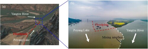
Confluences are critical nodes in a river network involving complex three-dimensional flow dynamics and bed morphological features, and serve important ecological functions (Boddy et al., 2019; Gualtieri et al., 2020; Yuan et al., 2022a). The confluence between the Yangtze River and the Poyang Lake outflow has an important role in mitigating flood, managing water resources and protecting the water environment and ecology in the Yangtze River Basin (Li et al., 2021a; Yuan et al., 2021). This confluence has a large floodplain on the internal side of the Poyang Lake outflow channel. During low flows this channel acts as a single channel; for high flow conditions it acts as a compound channel (Fig. 1) and significantly impacts the confluence hydrodynamics and morphodynamics. Similar topographic features can be also found in the confluence of the Yangtze River and Dongting Lake. Previous studies have mainly dealt with the dynamics in concordant or discordant-bed confluences. However, the effect of floodplain on confluence dynamics has not been systematically investigated so far through a physical model under well-controlled laboratory flow conditions.

Figure 1 A remote sensing image (a) and a drone image (b) of the confluence between the Yangtze River and the Poyang Lake with a large floodplain located on the internal side of the Poyang Lake outlet channel

The earliest studies on confluences dealt with flow hydrodynamics in laboratory flumes (Mosley, 1976). A conceptual model consisting of six distinct hydrodynamic regions was proposed by Best (1987): stagnation, shear layers, deflection, separation, maximum velocity, and flow recovery zones. Of interest was the separation zone (Best & Reid, 1984; Schindfessel et al., 2017; Yang et al., 2009) and the shear layer (Biron et al., 2019; Browand, 1986; Constantinescu et al., 2012; Rhoads & Kenworthy, 1998; Rogers & Moser, 1992; Yuan et al., 2018, 2022b; Zhang et al., 2020). The separation zone develops in the receiving channel near the downstream junction corner where the incoming flow from an angled tributary has sufficient momentum to detach from the channel wall (Biron et al., 1996a, 1996b; Yang et al., 2009). The size of the separation zone increases with increasingly dominant tributary inflow in an open channel confluence (Laurent et al., 2015). This zone involves recirculating fluid, which is common in laboratory flumes with sharp angled junction corners, but rarely exists in many natural confluences where junctions are often rounded or flared.

The shear layer of the confluence takes place where there is a significant velocity gradient and has been viewed as analogous to a plane shear layer that forms when two parallel flows begin to pass over one another downstream (Browand, 1986; Cheng & Constantinescu, 2021; Rogers & Moser, 1992). Proust et al. (2017) found the instability of the shear flow resulted in the development of Kelvin–Helmholtz (KH) structures, which are dependent on the velocity ratio between the two streams. The KH structures cannot form if (U₂ – U₁)/(U₂+ U₁) < 0.3 (Proust & Nikora, 2020), where U₁ and U₂ are the characteristic velocities of the two streams. These vertically orientated and co-rotating vortices can be identified in the energy spectra, especially when the spectra of transverse velocities for the shear layer near the water surface exhibit a characteristic “hump” at a low frequency (Rhoads & Sukhodolov, 2004; Yuan et al., 2016). In addition, Sukhodolov et al. (2010) extracted the scale of vortices in shear layers by observing the time of first local maxima of the auto-correlation functions, and their results showed that there was a positive correlation between time and the strength of vortices. However, if the momentum ratio between the tributaries was ∼1 and the shear along the margins of the stagnation zone was strong. Constantinescu et al. (2012) found that quasi two-dimensional eddies with opposing sense of rotation like wake vortices were created. Herrero et al. (2016) also found that a well-developed stagnation zone acted like a solid cylinder in a shallow open channel flow, leading to the vortex shedding like von Karman vortex street. Recent work by Sukhodolov et al. (2022) provided a theory that confluence mixing dynamics of shallow flows in which the mixing process is controlled by the switching between two modes of behaviour – KH versus wake mode.

Helical motion is another notable hydrodynamic feature at confluences (Best & Roy, 1991; Mosley, 1976; Rhoads & Kenworthy, 1998; Rhoads & Sukhodolov, 2001; Sukhodolov & Sukhodolova, 2019; Xu et al., 2022; Yuan et al., 2022b). The generation of helical cells at concordant confluences is attributed to the imbalance between centrifugal and pressure-gradient forces in space, similar to what is observed in meander bends (Rhoads & Johnson, 2018; Rhoads & Kenworthy, 1995). If two tributaries are angled to the post-confluence channel, the mutual flow deflection of the two streams causes dual counter-rotating secondary circulations (Ashmore et al., 1992; Mosley, 1976). If only one tributary is angled, the mutual flow deflection of the two streams produces opposing patterns of secondary circulation at confluences; however, twin surface-convergent helical cells rapidly evolve into a single circulation cell, as wide as the channel, due to the difference in the curvature of the two incoming flows (Bradbrook et al., 2000; Rhoads, 1996).

Field investigation has shown that a significant number of confluences are distinctly discordant, the tributary bed level being higher than that of the main channel (Canelas et al., 2020, 2022; Guillen-Ludena et al., 2015, 2017a, 2017b; Kennedy, 1984; Leite Ribeiro et al., 2012; Sukhodolov et al., 2017). Best and Roy (1991) reported that bed discordance modified flow structure, creating a distortion of the shear layer and fluid upwelling at the downstream junction corner, while near the bed the flow separation zone was missing. Bed discordance significantly enhanced the intensity of secondary circulation, caused by flow separation in the lee of the step (Biron et al., 1996a, 1996b; Bradbrook et al., 2001). Guillen-Ludena et al. (2015) observed that the upwelling flow at a movable bed discordant confluence contributed to the presence of a zone of reduced velocities instead of the flow separation zone. Numerical simulations demonstrated that the degree of bed discordance also influenced the mutual deflection of two flows and turning of the tributary flow became smaller and less pronounced with increasing difference in bed elevation (Dordevic, 2013; Ramos et al., 2019). Sukhodolov et al. (2017) showed that if the bed step was large and the higher-speed incoming tributary flow was akin to a jet, a secondary motion occurred downstream of the tributary junction, probably promoting the scour hole. The flow dynamics at the discordant confluence are also affected by the width ratio (the width of the tributary divided by that of the main channel), discharge ratio and junction angle (Guillen-Ludena et al., 2016, 2017b).

Compound open-channels have two-stage geometry: a main channel and adjacent floodplains that often have different width in the streamwise direction. As a result of different flow depths, composite hydraulic roughness and velocity differential between the main channel and the floodplain, complicated flow structure, involving large mixing layers, KH structures and secondary currents, develops (Dupuis et al., 2017; Kang & Choi, 2006; Knight & Demetriou, 1983; Myers et al., 2001; Singh et al., 2020; Truong & Uijttewaal, 2019). Furthermore, flow structure is generally affected by the shape of the floodplain, the relative depth, and relative velocity (Hamidifar et al., 2016; Proust et al., 2017). In a compound channel, the velocity ratio between the main channel and the floodplain drives KH structures and the direction and magnitude of the transverse flow, which modifies the number and size of the secondary currents (Proust & Nikora, 2020). Keshavarzi and Hamidifar (2018) identified the angle of convergence, the relative depth of flow and the width ratio in a compound channel as the variables controlling the values of the kinetic energy correction coefficient α and momentum correction coefficient β, which were related to the degree of the non-uniformity of the velocity.

Despite the extensive work on the hydrodynamics of channel confluences, few, if any, studies have examined the influence of floodplains at confluences on flow dynamics including the influence of floodplains on three-dimensional velocity field, helical cells, separation zone and shear layers. Such understanding is relevant also to the ecological quality of the aquatic environment at a river confluence (Blettler et al., 2015). Many rivers, especially those in lowlands, as conditions on the Yangtze River demonstrate confluences with a floodplain exist, and the effects of the floodplain need to be fully explained. The present study represents a first step toward addressing this issue by examining a particular confluence floodplain configuration where the tributary channel has a floodplain. Through laboratory experiments, this study aims to investigate the effects of the floodplain in the tributary on the confluence hydrodynamics, i.e. three-dimensional mean velocity field, spanwise uniformity of flow velocity distribution, turbulent characteristics, strength and scale of secondary currents, and size of flow separation zone.

2 Experimental set-up and measurement

The experiments were carried out at the Laboratory of Sediment of Hohai University (China) in a confluence flume (Fig. 2a). The straight upstream channels were both 3 m long, 0.32 m wide and 0.4 m deep, while the post-confluence channel was longer (7 m) and slightly wider (0.42 m). The junction angle was 60° and the confluence had a concordant bed. Two different geometrical configurations were considered. In Geometry no. 1 the three channels had simple rectangular cross-section, whereas in Geometry no. 2 a cuboid of Plexiglas plates was placed in the tributary channel to simulate a floodplain located on the left side. The width and height of the floodplain were 0.16 m and 0.1 m, respectively (Fig. 2a).

Figure 2 Sketch of a confluence channel flume with the floodplain (a) and measurement grid: (b) plan view; (c) cross-sectional points of measurement. Geometries no. 1 and no. 2 represent the cases without and with the floodplain, respectively. The circles and triangles represent some measurement points for the energy spectrum analysis for Geometries no. 1 and no. 2, respectively. (All distances are normalized as X = x/W, Y = y/W and Z = z/h)

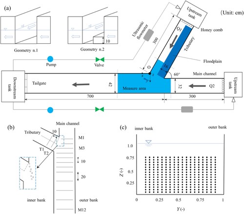
Flow was pumped from the downstream tank to two upstream tanks through polyvinyl chloride pipeline, and the flow rate was closely regulated by two pump-valve systems and ultrasonic flowmeters (accuracy ± 0.01 l s⁻¹). Honeycombs and sufficiently long channels were used to ensure fully developed flows entering the junction point. The downstream junction was selected as the origin of the coordinates and the orientation of coordinate axes (x, y, z) is shown in Fig. 2a.

Figure 2b shows the velocity measurement zone of each cross section. Detailed three-dimensional velocity measurements were carried out at two cross sections (T1 and T2) in the tributary and at 12 cross sections (M1, M2, … M12) in the main channel (Fig. 2b). The distance between each cross section was 10 cm in the tributary, as well as in the main channel from M1 to M8, while from M8 to M12 the distance between sections was increased to 20 cm (Fig. 2b). In each cross section, the transverse spacing of the measured profiles was 2 cm, and the interval between two adjacent vertical measurement points was 1 cm (Fig. 2c). Furthermore, four additional measurement locations were considered for the energy spectrum analysis within the shear layer (Fig. 2b).

Two experiments were carried out for identical flow conditions: the discharges in the tributary and in the main channel were 7 l s⁻¹ and 10 l s⁻¹, respectively, yielding a discharge ratio (Q_r= Q_t/Q_m) of about 0.7. The water level was adjusted by the tailgate, and the water level was fixed as 20 cm at 0.5 m upstream of the tailgate. The bulk velocity in the tributary was 0.11 m s⁻¹and 0.15 m s⁻¹ for Geometry no. 1 and Geometry no. 2, respectively. The overall flow parameters are summarized in Table 1.

Table 1 Flow conditions of the experiments

Cases	h (m)	Qt (l s^−1)	Qm (l s^−1)	Qr (–)	Vt (m s^−1)	Vm (m s^−1)	Ft (–)	Fm (–)	Ret (–)	Rem (–)	Mt (kg m s^−2)	Mm (kg m s^−2)	Mr (–)
Geometry no. 1	0.2	7	10	0.7	0.11	0.16	0.08	0.11	9722	13889	0.77	1.56	0.49
Geometry no. 2	0.2	7	10	0.7	0.15	0.16	0.10	0.11	9722	13889	1.02	1.56	0.65

Note: including the Reynolds number, R_e= uR/v, where u is the flow velocity, R is hydraulic radius and v is the water kinematic viscosity, the Froude number, F = u/(gh)^1/2, where h is flow depth, and the momentum flux, M=ρuQ. The subscripts of “m” and “t” represent the main channel and the tributary, respectively. M_r is the ratio of flow momentum, M_r= M_t/M_m.

Three-component instantaneous velocities were acquired using an acoustic Doppler velocimeter at a sampling frequency of 100 Hz for 120 s per point (ADV, Nortek Vectrino+, Oslo, Norway; maximum velocity: 4 m s⁻¹; accuracy: ± 10⁻³ m s⁻¹). For comparison, Biswal et al. (2016) measured three-component point velocities at a sampling rate of 50 Hz and a duration of 180 s, while Canelas et al. (2020) measured three-component point velocities across 13 sections at a sampling rate of 100 HZ for 90 s.

Silica powder was added to the water to improve signals from the ADV. The manufacturer, Nortek, specifies the minimum acceptable correlation value as 70% (Canelas et al., 2020). The method for detecting spikes using the phase space threshold proposed by Goring and Nikora (2002) was used in this study; the points were enclosed by an ellipsoid defined by the universal criterion, and the points outside the ellipsoid were designated as spikes, which enhances the high-frequency part of a signal. The accuracy of the time-averaged flow velocities using ADV was better than 4% (Lemmin & Rolland, 1997). The ADV instrument’s noise of different receivers is statistically independent, which indicates that the estimates of turbulent shear stresses are noise-free. The noise may cause indeterminacy of about 20% in the turbulent normal stresses and the turbulent kinetic energy (Blanckaert, 2010).

3 Results and discussion

3.1 Stationarity analysis

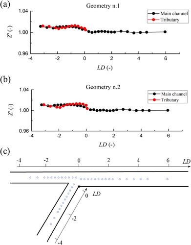
Figure 3 shows the profile of water surface at the centre of channel in two cases. The maximum difference of flow depth of two cases was 0.7 mm, which is about 0.35% of flow depth. Thus, the effect of the floodplain on the flow depth longitudinal profile was minor.

Figure 3 The profile of water surface at the centre of channel in Geometries no. 1 case (a) and no. 2 case (b), and image (c) shows where LD is the non-dimensional longitudinal coordinate with the zero value at the corner. The water level was measured using a point gauge with an accuracy of ± 0.1 mm

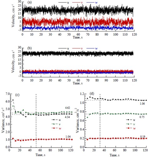
The stationarity analysis of the velocity data is usually used to check the accuracy of measurement duration (Sukhodolov & Rhoads, 2001; Yuan et al., 2016). In the present study each time series (Fig. 4a and b) was divided into 24 equal intervals, and their variance was progressively cumulated over the 24 intervals (Fig. 4c and d). The systematic convergence of the cumulative variance to a constant value is indicative of a stationary variance. Hence, the record length was sufficient to capture major sources of variation in velocity. The plots for the shear layer and ambient flow exhibited convergence. The record length was defined to be equal to 90% of the long-term mean-variance. By serving as sampling intervals for the flow measurements, these values were 30 s for the ambient fluid and 50 s for the shear layer (Fig. 4c and d).

Figure 4 Examples of time series (a and b) and stationarity analysis (c and d) of 3D velocities within and outside the shear layer in M4; the coordinates are (3, 16, 10) and (3, 34, 14), respectively

3.2 Three-dimensional velocity field

Figure 5 shows the distribution in the plane yz of velocity vectors (v, w) superimposed on the contours of the streamwise velocities u in the tributary for both cases. In Geometry no. 1, the streamwise velocity and secondary flow velocity in the tributary all increased from T1 to T2 (Fig. 5a and c), due to being affected by the higher-speed main channel flow. In Geometry no. 2, the typical flow structure of a compound channel in T1 was observed (Fig. 5b), characterized by the difference of flow velocity between the tributary main channel and floodplain and the secondary motions (Dupuis et al., 2017; Knight & Demetriou, 1983). However, this structure was modified near the confluence zone. The streamwise velocity in the tributary main channel increased from T1 to T2 (Fig. 5d), while the velocities over the floodplain in T1 and T2 were similar. The values of secondary flow velocity in T2 exceeded those in T1 by a factor of 2–3. All the vectors were pointed towards downstream, which was similar with the observation in Geometry no. 1. Furthermore, the main effects of the floodplain were to reduce the cross-sectional area of the tributary flow and increase velocities of flow entering the main channel from the tributary.

Figure 5 Distribution in the plane y′−z′ of contours of streamwise velocities u′ and the vectors of velocities (v′, w′), in the tributary for Geometry no.1 (left) and Geometry no.2 (right). u, v and w are the three components of flow velocity in the new reference axes, X′ (along with the tributary flow) and Y′ (point to floodplain side) are normalized by W, and Z′ (in the vertical direction) is normalized by h, respectively. (a) and (b) represent the T1 cross section; (c) and (d) represent the T2 cross section.

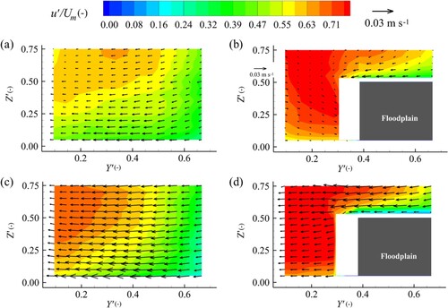
Figure 6 shows the cross-sectional distribution of the time-averaged velocity components for both Geometry no. 1 and no. 2 using Tecplot360, where u, v and w stand for the three components of velocity in the reference axes, X, Y and Z, respectively.

Figure 6 Spatial distribution of 3D velocity at different measurement cross sections for Geometry no. 1 (a, c, e) and Geometry no. 2 (b, d, f)

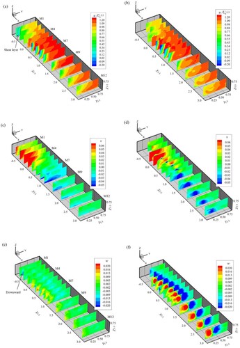
The u-field for Geometry no. 1 (Fig. 6a) shows that M1 lies within the stagnation zone near the upstream junction corner, where the velocity was nearly zero. The main channel and the tributary both increased their streamwise velocity in the confluence zone. Subsequently, two higher-speed zones appeared from M4 to M6 due to the mutual interaction of flows and the occurrence of the separation zone. Negative streamwise velocities were observed near the inner bank of M5 and farther downstream (M6–M8), indicative of the presence of the separation zone. Yang et al. (2009) proposed to identify the downstream boundary of the separation zone using the mainstream isovel with zero velocity. The layer (black ovals) with the largest velocity gradient was nearly vertical in M1 and M2, indicating the location of the shear layer (Yuan et al., 2016).

In Geometry no. 2 (Fig. 6b), the floodplain divided the tributary flow into higher-speed flow in the channel and lower-speed flow on the floodplain. In addition to the two higher-speed zones observed in Geometry no. 1 (Fig. 6a), a third higher-speed zone was noticed at the interface between the two merging flows. A flow separation zone with negative streamwise velocity appeared at downstream junction corner.

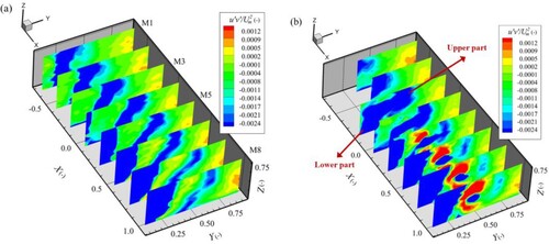
The spatial distribution of v-velocity in Geometry no. 1 (Fig. 6c) showed that from M2 to M5 the positive lateral velocity region had a triangular shape as the tributary flow tended to invade the main channel flow, especially near the water surface. The positive velocities near the water surface gradually decreased from 0.06 m s⁻¹ in M2 to 0.02 m s⁻¹ in M8. Simultaneously, the magnitude of negative velocities near the bed gradually increased from −0.02 m s⁻¹ to −0.05 m s⁻¹, indicating a helical motion. In Geometry no. 2 (Fig. 6d), a zone of negative v-velocities larger than in Geometry no. 1 appeared near the bed at M7. The zone of negative velocities near the bed gradually moved away from the inner side and then moved back to the inner side again from M3 to M12. It is noteworthy that the negative lateral velocity zone near the bottom existed for a longer downstream distance than in Geometry no. 1, which was attributed to the occurrence of much stronger secondary circulation.

In the w-velocity plot in Geometry no. 1 (Fig. 6e), the downward flow was in accordance with the large velocity gradient in the u-field plot, indicating the shear layer between the two flows. Upwelling and downward flows occurred near both sides of the main river channel and they gradually became weak. In Geometry no. 2 (Fig. 6f), the upwelling and downward flows were visible and more intense compared to those in Geometry no. 1. The strong upwelling was also observed downstream of tributary corner in discordant confluences studied by Biron et al. (1996a, 1996b). It is believed that this upwelling was enhanced by flow separation in the lee of the bed step of a discordant confluence or, in our study, by the floodplain step, which significantly increased the lateral pressure gradient at the bed (Bradbrook et al., 2001). Moreover, as suggested by De Serres et al. (1999), this upwelling motion might create patterns of mean flow indicating persistent secondary circulation.

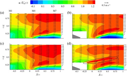
The additional higher-speed zone can be clearly identified by comparing the lower flow of Geometry no. 2 (Fig. 7d) to that in Geometry no. 1 (Fig. 7c). This zone was primarily caused by the interaction of flow between the main channel and the floodplain, but it did not exist in the upper flow region (Fig. 7b). This interaction should be related to the convergence of flow near the bed from the tributary and the main channel, as seen by the biased vectors in this zone showing local flow convergence in Fig. 7d. The higher-speed zone disappeared in M7 due to the weakening of such expansion.

Figure 7 Time-averaged mean velocities of Geometry no. 1 (left) and Geometry no. 2 (right), contours for spatial distributions of velocities and u, v (vectors) in the xy plane (M1–M8): (a) and (b) Z = 0.7; (c) and (d) Z = 0.4. Encircled area represents the region of higher-speed flow

3.3 Size and time/length scale of secondary motion

The present study adopted the Rozovskii definition to identify secondary circulation produced by helical motions, and this method has been widely used in the strongly converging flows (Rhoads & Kenworthy, 1998; Rozovskii, 1957; Szupiany et al., 2009; Yuan et al., 2021). Each vertical ensemble of velocity data is rotated in the Rozovskii reference frame so that the primary and secondary velocity components are parallel and perpendicular to the orientation of the depth-averaged velocity vector, respectively. Figure 8 shows the secondary flow velocity distribution in M4 using the Rozovskii definition for Geometry no. 2, where an evident secondary cell can be identified. The upper layer flow with positive lateral velocity had a lower streamwise velocity, and the lower flow with the negative lateral velocity had a larger streamwise velocity. This secondary cell, which exhibited clockwise circulation when viewed in the upstream direction, is likely related to the streamline curvature of the tributary flow as suggested by previous work (e.g. Rhoads & Kenworthy, 1998; Yuan et al., 2021). Furthermore, the local lateral expansion of the main channel flow near the bed caused by the floodplain step enhanced the secondary motion that persisted for a longer distance downstream (X > 3).

Figure 8 Contours for non-dimensional streamwise velocities and vectors of cross-sectional velocities (v, w) in M4 in Geometry no. 2. The figure is looking upstream

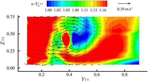
Figure 9 shows the vectors of secondary flow at different locations downstream of the junction using the Rozovskii definition in both Geometry no. 1 and Geometry no. 2. In the present study, only one helical cell was observed in both cases. In Geometry no. 1, a clockwise helical cell was observed near the bed at Y = 0.2–0.4, Z = 0.2–0.3 (Fig. 9a and c), which could possibly reflect helical motion generated by the streamline curvature. Since it was located very close to the channel corner, wall effects that resulted in turbulence anisotropy could also influence helicity (Nezu et al., 1993). The circulation velocity ranged from 0.01 m s⁻¹ to 0.03 m s⁻¹ at M5 and M6 (Fig. 9a and c). In Geometry no. 2, the size and intensity of helical cell was clearly larger and its velocity reached 0.05–0.06 m s⁻¹ (Fig. 9b and d), which should be related to the flow expansion from main channel/fluid upwelling in the lee of the floodplain step. In addition, the higher momentum ratio suggested that velocities in the tributary were also higher (Table 1), which should increase helicity by amplifying the centrifugal force. The helical cell was located at Y = 0.30–0.60 at M6, occupying almost one-third of the cross section.

Figure 9 Secondary velocity (vectors) of Geometry no. 1 (left) and Geometry no. 2 (right): (a) and (b) represent the M5 cross section; (c) and (d) represent the M6 cross section. The red arrows represent the secondary motions. These figures are looking upstream

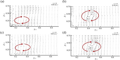
Table 2 lists the rotational velocity, the width as well as the time/length scale for a complete rotation of the helical cells observed in the present study. It is apparent that the alternate flow mechanism (single channel/compound channel) in the tributary significantly affected the secondary motion at the confluence. In Geometry no. 1, a clockwise secondary motion having a rotational velocity of 0.02 to 0.03 m s⁻¹ and a width of 0.10 to 0.12 m, completing a rotation in about 14 s was observed. In Geometry no. 2, the rotational velocity and the width of such cell increased, due to the higher-speed flow of non-floodplain side in the tributary and flow expansion of the main channel flow.

Table 2 Size and time/length scale for a complete rotation of helical cells

Cases	Rotational velocity (m/s)	Width (m)	Timescale for complete rotation (s)	Length scale for complete rotation (m)
Geometry no. 1	0.02–0.03	0.10–0.12	14	3.0
Geometry no. 2	0.03–0.05	0.12–0.14	10	2.3

3.4 Flow separation zone

The separation zone, often characterized by recirculation with low velocities, is an important feature of the post-confluence channel. Its size and location have a significant impact on sediment transport and pollutant dispersion in the confluence zone (Biron et al., 1996a, 1996b).

The size of the flow separation zone was roughly defined by its width W_s and length L_s. The values of these parameters can be determined straightforwardly from the complex three-dimensional flow pattern. Different methods of identifying the separation zone have been proposed in the literature. The zero-discharge method, streamline method and isovel method were adopted in the previous studies (Best & Reid, 1984; Gurram et al., 1997; Yang et al., 2009; Schindfessel et al., 2017). In the present study the isovel method was used, where the isoline of zero longitudinal velocity was applied to define the size of the separation zone. As this method was implemented in a horizontal plane, whereas the separation zone was known to have a three-dimensional structure, different horizontal planes were considered. They were located at Z = 0.15, 0.45 and 0.75, identifying the separation zone over the depth, as suggested by Best and Reid (1984), Gurram et al. (1997) and Schindfessel et al. (2017).

Table 3 lists the size (width and length) of the separation zone on horizontal planes at the different depths. The separation zone was also identified on the velocity plots in Fig. 9. Table 3 demonstrates that the separation zone was near the surface wider and longer than near the bed for both geometries. This result was consistent with previous studies (Best & Reid, 1984; Schindfessel et al., 2017). In their LES studies, Schindfessel et al. (2017) found that the width of the separation zone was about 0.1W–0.3W, and the length near 1.8W (W was the width of the post-confluence channel), which agreed well with the present experimental results (Table 3). Near the bed the width of the separation zone was similar for the two geometries, but the difference between the two gradually increased over the depth. At Z = 0.75 the width was 0.16W and 0.20W in Geometry no. 1 and Geometry no. 2, respectively. Such larger width of the separation zone might be related to the larger momentum ratio of the flow for Geometry no. 2., which led to a stronger flow deflection downstream of the junction. However, it was interesting that the length of the separation zone was similar for the geometries, as the length of the separation zone was mainly related to the discharge ratio and junction angle.

Table 3 Dimensions of the separation zone at different depths

Cases	Z (–)	Ws/W (–)	Ls/W (–)
Geometry no. 1	0.15	0.10	0.19
	0.45	0.14	0.95
	0.75	0.16	1.19
Geometry no. 2	0.15	0.10	0.21
	0.45	0.15	0.95
	0.75	0.20	1.24

Figure 10 shows the vectors of longitudinal-vertical plane velocities (u,w) superimposed on the contours of streamwise velocities u for the two geometries in the channel reach from M5 to M10. In Geometry no. 1, negative, low streamwise velocities and velocity vectors were spread over the entire depth at Y = 0.10. The streamwise velocity gradually increased laterally at the bottom but remained small at the top at Y = 0.14 and 0.19, confirming that the width of the separation zone was larger at free-surface than at the bottom. Yang et al. (2009) compared the separation zones on the vertical plane and found that at the bottom the separation zone reduced in width by the secondary flow, even to the degree that it was entirely eliminated.

Figure 10 Time-averaged velocities of Geometry no. 1 (left) and Geometry no. 2 (right), contours for spatial distributions of velocities and u, w (vectors) in the xz plane of the separation zone, (a) and (b) Y = 0.10; (c) and (d) Y = 0.14; (e) and (f) Y = 0.19; (g) and (h) Y = 0.24. The red ovals represent the region of unrecovered separation

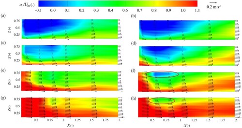
In Geometry no. 2, the velocity distribution was similar to that in Geometry no. 1 at Y = 0.10 and 0.14. However, the strong upwelling, due to the bed discordance, was mainly concentrated on the downstream junction corner. Here the main channel flow could pass smoothly along the sidewall of the step and destroy the separation zone near the bed (Biron et al., 1996a, 1996b; De Serres et al., 1999; Guillen-Ludena et al., 2015). The flow on the deep channel of the tributary entered near the bed, leading to curved streamline over the entire depth. Fluid upwelling appeared near the step of the floodplain and expanded towards the middle of the main channel (Fig. 6f), not impacting on the separation zone near the bed. The lower streamwise velocity and velocity vectors (red ovals in Fig. 10f and h) indicated that the flow was not recovered, especially in the upper layer at Y = 0.19 and 0.24.

3.5 Kinetic energy and momentum correction coefficients

Kinetic energy correction coefficient α and momentum correction coefficient β are commonly used to quantify the degree of the non-uniformity of velocity distribution in open channel flows (Chow, 1959). They were also used in laboratory confluences by Hsu et al. (1998a, 1998b). The two coefficients are defined as: (1) $\begin{array}{rl}\alpha & =\frac{{\displaystyle {\int }_A{v}^{3}dA}}{v_{vae}^{3}A}\end{array}$(1) (2) $\begin{array}{rl}\text{β}& =\frac{{\displaystyle {\int }_A{v}^{2}dA}}{v_{vae}^{2}A}\end{array}$(2) where v is point-velocity in the cross section, v_vae is the cross-sectional mean velocity, A is the cross-sectional area, and dA is an elementary area of the cross section. The correction coefficients (α and β) are strictly equal to 1 if the velocity is uniformly distributed; generally they are larger than 1 in natural streams, where the velocity distribution is non-uniform (Chanson, 2004). In laboratory confluences, Hsu et al. (1998a) found that α and β decreased as the discharge from the tributary increased and attained a local maximum at a downstream location, which was at a distance of twice the width of the channel. In addition, α and β were found to depend upon the discharge ratio, the junction angle and the downstream channel geometry (Hsu et al., 1998a, 1998b; Ramamurthy et al., 1988).

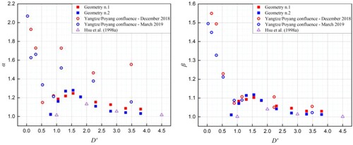
Figure 11 shows the comparison of our experimental results, the flume-experimental data of Hsu et al. (1998a) and the field survey data of Li et al. (2022b). Data of Hsu et al. (1998a) were for a confluence without floodplain. Li et al. (2022b) data were for two field surveys: one with a non-submerged floodplain (December 2018) and one with submerged floodplain (March 2019). In our study, the values of α and β tended first to increase and then decayed as the distance from the junction increased, which were generally in agreement with the results of Hsu et al. (1998a). The maximum values of α and β in Geometry no. 2 were larger than those in Geometry no. 1, probably due to the three higher-speed velocity zones and the wider separation zone (negative velocity zone) at the downstream junction corner, where the flow velocity was more non-uniform. However, farther downstream in Geometry no. 2, α and β values decayed, indicating that the floodplain enhanced flow recovery in the post-confluence channel. In addition, both in the present study and at the Yangtze River/Poyang Lake confluence α and β peaked immediately downstream of the junction at D′ = 1.2–1.5. However, it was believed that the root-cause of such local peaks was different. In the present study, this peak was likely related to the flow separation zone; while at the Yangtze River/Poyang confluence it was mainly driven by the curvature of the post-confluence channel.

Figure 11 Longitudinal distribution of α and β at downstream of the confluence junction. D′=D/B, where D is the distance between the cross section and the junction apex, and B is the width of the cross section

3.6 Turbulent kinetic energy

The distribution of turbulent kinetic energy (TKE) within a cross section helps to identify the time-averaged structure of turbulence, like the separation zone, shear layer and secondary motions. An increased level of TKE (Fig. 12) takes place in the for mentioned zones. Turbulent kinetic energy can be calculated as: (3) $k=\frac{1}{2n}\sum _{i=1}^n(u_i^{\mathrm{\prime }}{u}_i^{\mathrm{\prime }}+v_i^{\mathrm{\prime }}{v}_i^{\mathrm{\prime }}+w_i^{\mathrm{\prime }}{w}_i^{\mathrm{\prime }})$(3) where $u_i^{\mathrm{\prime }}=u_i-\overline{u}$, $v_i^{\mathrm{\prime }}=v_i-\overline{v}$ and $w_i^{\mathrm{\prime }}=w_i-\overline{w}$ are the fluctuating velocity components based on the Reynolds decomposition, u_i, v_i and w_i are the component of instantaneous velocity (i = 1, 2 or 3), and $\overline{u}$, $\overline{v}$ and $\overline{w}$ are their time-average values.

Figure 12 Spatial distribution of non-dimensional TKE at different measurement cross sections for two cases: Geometry no. 1 (a) and Geometry no. 2 (b)

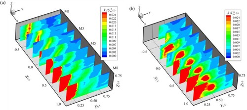
Figure 12 shows the normalized turbulence kinetic energy $k/U_m^2$, at different measurement cross sections for Geometry no. 1 and Geometry no. 2. In Geometry no. 1, the shear layer can be identified by a vertical band with large values of k that exceed those for the ambient flow by a factor of 3–5 (Rhoads & Sukhodolov, 2008; Sukhodolov & Rhoads, 2001). This region generally coincided with the large streamwise velocity gradient zone and downward flow (Fig. 6). This band expanded downstream and was inclined considerably, indicating that the main channel flow, more likely, enters the tributary flow near the bed. Strong turbulence near the tributary-channel side defined the flow shear bounding the separation zone (M5–M8), and this boundary was consistent with the zero-velocity definition and gradually moved outward downstream. In Geometry no. 2, the secondary circulation accompanied by high turbulence (M5–M8) was due to the higher mean velocity of the tributary flow and the flow expansion of the main channel flow, and the values of k were larger than those within the shear layer. The shear layer was vertical near the water surface of main channel. In Geometry no. 2, the width of separation zone was larger than that in Geometry no. 1, probably due to the larger velocity of the right-side of the tributary flow in the presence of the floodplain and, thus, to the larger deflection of the tributary flow.

3.7 Reynolds stresses

The distribution of the Reynolds stress ($-\rho u_i^{\mathrm{\prime }}{u}_j^{\mathrm{\prime }}$), i.e. correlations between velocity components, reflects the occurrence of time-averaged vortices or eddies in the plane. 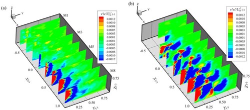It can be defined as the covariance of $u_i^{\mathrm{\prime }}$ and $u_j^{\mathrm{\prime }}$: (4) $<u_i^{\mathrm{\prime }}{u}_j^{\mathrm{\prime }}>=cov(u_i,u_j)=\frac{1}{n}{\sum }_{i=1}(u_i-\overline{u_i}\left)\right(u_j-\overline{u_j})$(4) Figure 13 shows the normalized Reynolds shear stress $<u^{\mathrm{\prime }}{v}^{\mathrm{\prime }}>/U_m^2$, at different measurement cross sections in Geometry no. 1 (Fig. 13a) and Geometry no. 2 (Fig. 13b). The shear layer with coherent turbulent structure in the horizontal plane could be identified as the regions with a large value of <u′v′> (Rhoads & Sukhodolov, 2008), where the shear layer has quasi-two-dimensional vortices around vertical axes that extends through the flow depth and inclines over distance downstream (Browand, 1986). In Geometry no. 1, large negative values of <u′v′> were found in a vertical band from Y = 0.19 in M1 to Y = 0.29 in M2, where the two flows merged, indicating the location of shear layer (Best, 1987; Yuan et al., 2016). The regions with large negative values of <u′v′> in Fig. 13 were coincident with those having large positive values of k in Fig. 12. These regions could be used to accurately identify the location and size of the separation zone and the shear layer.

Figure 13 Spatial distribution of non-dimensional Reynolds shear stress <u′v′> at different measurement cross sections for two cases: Geometry no. 1 (a) and Geometry no. 2 (b)

In Geometry no. 2, there was a distorted shear layer in M3 and M4, due to the expansion of the flow from the main channel to the tributary side. Its lower part deviated laterally by about 0.12 m from the upper part within M3. The upper part of the shear layer expanded downstream and decreased in intensity considerably. The lower part of the shear layers was destroyed by the secondary motions and disappeared in M5, as observed at discordant confluences (Biron et al., 1996a, 1996b; Sukhodolov et al., 2017). In addition, distortion of the shear layer can be related to many other reasons, such as a strong lateral penetration by the tributary (Yuan et al., 2016), helical motion (Constantinescu et al., 2012; Lewis & Rhoads, 2015; Rhoads & Kenworthy, 1995; Rhoads & Sukhodolov, 2001) and the density difference between the tributaries (Gualtieri et al., 2018, 2019; Horna-Munoz et al., 2020).

Figure 14 shows the normalized Reynolds shear stress $<v^{\mathrm{\prime }}{w}^{\mathrm{\prime }}>/U_m^2$, at different measurement cross sections for Geometry no. 1 (Fig. 14a) and Geometry no. 2 (Fig. 14b). In Geometry no. 1, large values of <u′w′> were observed in the middle of the shear layer as well as in the separation zone, consistent with the TKE distribution. In Geometry no. 2, large negative values of <u′w′> were located near the channel centreline, indicating that floodplain significantly enhanced the intensity and expanded the area of influence of the flow turbulence. Such secondary motions had an important impact on the mixing rates (e.g. Lyubimova et al., 2020).

Figure 14 Spatial distribution of non-dimensional Reynolds shear stress <u′w′> at different measurement cross sections for two cases: Geometry no. 1 (a) and Geometry no. 2 (b)

3.8 Autocorrelation function

The presence of regular coherent vortices in the shear layer can be identified through the auto correlation function of lateral velocity fluctuations v′. Based on the frozen turbulence hypothesis, this function can be calculated by using the values of one measured point at different lag times (Proust et al., 2017; Rhoads & Sukhodolov, 2004; Sukhodolov et al., 2010): (5) $R_{\tau }=\underset{T\to \mathrm{\infty }}{lim}\frac{1}{2T}{\displaystyle {\int }_{-T}^T{v}^{\mathrm{\prime }}(t+\tau )v^{\mathrm{\prime }}\left(t\right)\mathrm{d}t}$(5) where R is the autocorrelation function, τ is lag time, t is time, and T is a time period.

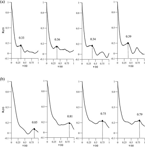
Figure 15 shows the representative profiles of the autocorrelation function of lateral velocity fluctuations v′ at different locations (Fig. 2b) for both Geometry no. 1 (Fig. 15a) and Geometry no. 2 (Fig. 15b). In Geometry no. 1, initially the autocorrelation function sharply decreased and then gradually increased to a maximum of about 0.35 s, indicating that the initial lateral velocity sequence has a high similarity with the velocity sequence at t = 0.35 s. The vortex periodicity for 0.35 s dominated the quasi-two-dimensional structure. In Geometry no. 2, the autocorrelation function rapidly decreased and then gradually increased, reaching a local peak at about 0.8 s. The dominant vortex in the shear layer was stronger, and the periodicity was twice that in Geometry no. 1. This may be explained by a large velocity gradient between the floodplain and the main channel flows, which generates a large quasi-two-dimensional vortex. Furthermore, there was no significant difference in the time when the autocorrelation function reached the first peak at different locations of the confluence. The dominant vortex does not appear to evolve substantially along the shear layer (Chu & Babarutsi, 1988; Uijttewaal & Booij, 2000).

Figure 15 Autocorrelation function R_τ: (a) Geometry no. 1 and (b) Geometry no. 2

3.9 Discussion on dynamics of confluence with floodplain

The typical, hydrodynamics features (e.g. Best, 1987; Mosley, 1976) were identified in Geometry no. 1 such as stagnation zone, deflection zone, separation zone with recirculation, maximum velocity zone, flow recovery zone and shear layer. The helical cell, observed in Geometry no. 1 (Fig. 9a and c), is also a common feature of confluence dynamics (e.g. Rhoads & Kenworthy, 1995, 1998; Bradbrook et al., 2000; Constantinescu et al., 2012). However, in Geometry no. 2, with the presence of floodplain, confluence dynamics were altered. Larger and more intensive secondary motions, a tilted shear layer, an additional higher-speed zone and a wider separation zone were observed. These experimental phenomena are different from concordant and discordant confluences (Bradbrook et al., 2001; Canelas et al., 2020).

Proust and Nikora (2020) suggested that in a compound channel the secondary flow reaching about 4% of the mean streamwise velocity was associated to turbulence anisotropy, but in cases of non-uniform flow with floodplains that produced flow toward the main channel, cells produced by turbulence anisotropy could be modified. Thus, the possible effects of secondary cell in the tributary compound channel on the secondary motions in the post confluence channel are also discussed. In our study, the flows from the floodplain toward the tributary channel were also observed in Geometry no. 2 (Fig. 5d). The secondary cell was observed in T1 in the tributary but disappeared in T2, and all the cross-sectional velocity vectors in T2 pointed downstream under the incoming high-speed main channel flow. That is, the effects of secondary cell were limited and mainly existed upstream of T2 in the tributary. Moreover, in the post-confluence channel the velocity of secondary motion reached 0.04–0.06 m s⁻¹ (Fig. 9b and d), i.e. about 20% of the primary flow velocity (U_m). Thus, these results suggested that the secondary cell in the tributary compound channel appears to be feeble in comparison to the secondary flow at the confluence, and its effects could be neglected.

In Geometry no. 1, a helical motion could be observed at the corner (Fig. 9a and c) and its velocity was about 8% of U_m. The velocity of the helical cells caused by the streamline curvature is about 10% of U_m at the post confluence channel (Ashmore et al., 1992; Yuan et al., 2021). Nezu et al. (1993) found that secondary currents at the corner could reach 2% of U_m caused by anisotropic wall turbulence in a straight channel. Hence, the production of secondary motion in Geometry no. 1 seems to be mainly associated to the streamline curvature, and the anisotropy of turbulence may also play a role in that motion. Due to the bed discordance, the lateral pressure gradients were significantly altered in the central confluence zone because of the flow separation over the step, and could also contribute to helical motion (Bradbrook et al., 2001). The dynamics are similar to those in Geometry no. 2, where the expansion of the main channel flow into the lee of the floodplain step was observed in M1 and M2 (Fig. 6b), indicating that the lateral pressure gradient at the bed was low, and then fluid upwelling was located downstream of the floodplain step (Fig. 6f). Moreover, a large momentum flux was found in Geometry no. 2 because the floodplain restricted the cross-sectional area. As the momentum flux from the lateral tributary increased, the curvature-induced helical motion expanded over the width of the downstream channel (Lewis & Rhoads, 2015). In summary, the secondary motion was mainly related to the flow expansion from main channel/fluid upwelling in the lee of the floodplain step and streamline curvature, with perhaps anisotropic wall turbulence also having an influence.

The expansion also induced the distortion of the shear layer and, subsequently, a different distribution of the turbulent energy (Fig. 12b) and Reynolds shear stresses (Fig. 13b). The shear layer in the Geometry no. 2 case had lower-frequency dominant K-H vortices as demonstrated by the auto correlation function of lateral velocity fluctuations, which reflected larger flow shear between the floodplain flow and the main channel flow. In addition, a wider separation zone related to the higher-speed inflow near the corner was found in Geometry no. 2, leading to a larger flow deflection, while the length of the separation zone was almost the same in the two geometries, as it depended on the discharge ratio. This structure was different from that in a discordant confluence where fluid upwelling can destroy the flow separation near the bed (Biron et al., 1996a, 1996b; Bradbrook et al., 2001; Dordevic, 2013). However, in the present study, due to the intervening tributary main channel flow, the upwelling caused by the floodplain step was far away from this zone and was ineffective at eliminating flow separation.

4 Conclusions

The hydrodynamic effects on confluence flow structure of the floodplain in one tributary were investigated through the analysis of detailed three-dimensional velocities and turbulent flow structures measured in a physical model. Two different geometries, i.e. where the tributary acted as a single-channel and as a compound channel due to the floodplain, respectively, were investigated under the same discharge ratio and downstream water depth. The confluence floodplain configuration where the tributary channel has a floodplain was observed at many rivers, particularly those in lowlands, and this study provides a beginning step toward addressing it. Several important conclusions can be drawn:

1. Flow hydrodynamics at a confluence with the tributary acting as a compound channel are characterized by an additional higher-speed zone, larger and more intensive secondary motions, a distorted shear layer, and a wider separation zone if compared with the corresponding hydrodynamics features observed in a single channel tributary.

2. The flow separation in the lee of the floodplain step significantly increased lateral pressure gradients at the bed, promoting a flow expansion from the main channel flow toward the tributary flow near the bed.

3. The additional higher-speed zone and helical cell could mainly be related to the flow expansion from main channel/upwelling in the lee of the floodplain step and higher velocities of flow from tributary. This cell was larger and more intense than that due to the flow curvature in the geometry without floodplain. The effects of secondary cell in the tributary compound channel on the secondary flow at confluence could be neglected.

4. The shear layer was characterized by increased turbulence levels and values of <u′v′> and it was distorted by the flow expansion and destroyed in its lower part by the helical cell.

5. The width of the separation zone was larger as the inflow from the non-floodplain side of the tributary had a larger momentum. However, the length of the separation zone was almost unchanged if compared with that in the single-channel case, as the length is more related to the discharge ratio. This structure is different from that in a discordant confluence where fluid upwelling can destroy the flow separation near the bed.

6. The values of the kinetic energy correction coefficient α and momentum correction coefficient β in the geometry with floodplain were generally larger than in the geometry without floodplain. This is probably due to the combined effects of the three higher-speed zones and the wider separation zone. These coefficients peaked downstream the junction and subsequently decreased. The floodplain might enhance momentum exchange between the merging flows.

7. In the floodplain geometry the dominant vortex in the shear layer had a frequency lower than that in the single-channel configuration, as demonstrated by the auto correlation function of lateral velocity fluctuations. This was likely due to the larger flow shear between the floodplain flow and the main channel flow.

8. The study gained novel information about hydrodynamics of confluences where one of the tributaries is acting as a compound channel due to a floodplain located on its inner bank. Hence, it is believed that the above presented results could be useful also to understand the complex hydrodynamics of the large confluence between the Yangtze River and the Poyang Lake, whose outlet channel is temporarily acting under high flow conditions as a compound channel. Moreover, many rivers have floodplains and this study is a first effort to account for the influence of floodplains on confluence hydrodynamics.

Notation

B	=	width of the cross section (m)
D	=	distance between the cross section and the junction apex (m)
F	=	Froude number (–)
g	=	gravity acceleration (m s-2)
h	=	water depth (m)
k	=	turbulent kinetic energy (m2 s−2)
LD	=	non-dimensional longitudinal coordinate (–)
M	=	momentum flux (kg m s−2)
Mr	=	momentum flux ratio (–)
Q	=	discharge (l3 s−1)
Qr	=	discharge ratio (–)
Rτ	=	autocorrelation function (–)
Re	=	Reynolds number (–)
t	=	time (s)
T	=	a time period (s)
Um	=	average flow velocity in post confluence channel (m s−1)
u, v, w	=	velocity components (m s−1)
u′, v′, w′	=	fluctuating velocity components (m s−1)
<u′v′>	=	Reynolds stress (m2 s−2)
<u′w′>	=	Reynolds stress (m2 s−2)
W	=	width of the post-confluence channel (m)
x, y, z	=	streamwise, lateral and vertical coordinate of main channel (m)
x′, y′, z′	=	streamwise, lateral and vertical coordinate of tributary (m)
X, Y, Z	=	non-dimensional distances in x, y, z directions, respectively (–)
X′, Y′, Z′	=	non-dimensional distances in x’, y’, z’ directions, respectively (–)
α	=	kinetic energy correction coefficient (–)
β	=	momentum correction coefficient (–)
τ	=	lag time (s)

Acknowledgements

The authors would like to thank Professor Bidya Sagar Pani of the Indian Institute of Technology-Bombay for help in revising this work. Thanks are also extended to Kang Chen, Qingwei Lin, Hao Lin, Mengyi Wang, Lei Xu, Kun Li, Yunqiang Zhu, Jiaming Yang and Yuchen Zheng of Hohai University for their support in the experiments.

Disclosure statement

No potential conflict of interest was reported by the author(s).

Additional information

Funding

This research is supported by the National Key R&D Program of China [grant no. 2022YFC3202602], the National Natural Science Foundation of China [grant 52079044; U2240209; U2040205], and the Fok Ying Tung Education Foundation [grant 520013312].

References

- Ashmore, P. E., Ferguson, R. I., Prestegaard, K. L., Ashworth, P. J., & Paola, C. (1992). Secondary flow in anabranch confluences of a braided, gravel-bed stream. Earth Surface Processes and Landforms, 17(3), 299–311. https://doi.org/10.1002/esp.3290170308
- Best, J. L. (1987). Flow dynamics at river channel confluences: Implications for sediment transport and bed morphology. In Recent developments in Fluvial Sedimentology, F. G. Ethridge, R. M. Flores, & M. D. Harvey (Eds.), 39 (pp. 27–35). Tulsa: SEPM Society for Sedimentary Geology. http://doi.org/10.2110/pec.87.39.0027
- Best, J. L., & Reid, I. (1984). Separation zone at open-channel junctions. Journal of Hydraulic Engineering, 110(11), 1588–1594. https://doi.org/10.1061/(ASCE)0733-9429(1984)110:11(1588)
- Best, J. L., & Roy, A. G. (1991). Mixing-layer distortion at the confluence of channels of different depth. Nature, 350(6317), 411–413. https://doi.org/10.1038/350411a0
- Biron, P. M., Best, J. L., & Roy, A. G. (1996a). Effects of bed discordance on flow dynamics at open channel confluences. Journal of Hydraulic Engineering, 122(12), 676–682. https://doi.org/10.1061/(ASCE)0733-9429(1996)122:12(676)
- Biron, P. M., Buffin-Bélanger, T., & Martel, N. (2019). Three-dimensional turbulent structures at a medium-sized confluence with and without an ice cover. Earth Surface Processes and Landforms, 44(15), 3042–3056. https://doi.org/10.1002/esp.4718
- Biron, P. M., Roy, A. G., & Best, J. L. (1996b). Turbulent flow structure at concordant and discordant open-channel confluences. Experiments in Fluids, 21(6), 437–446. https://doi.org/10.1007/BF00189046
- Biswal, S. K., Mohapatra, P. K., & Muralidhar, K. (2016). Transitional flow in a right-angled compound open canal junction. Irrigation and Drainage, 65(1), 73–84. https://doi.org/10.1002/ird.1943
- Blanckaert, K. (2010). Topographic steering, flow recirculation, velocity redistribution, and bed topography in sharp meander bends. Water Resources Research, 46(9), 2095–2170. https://doi.org/10.1029/2009WR008303
- Blettler, M. C., Amsler, M. L., Ezcurra de Drago, I., Espinola, L. A., Eberle, E., Paira, A., & Drago, E. E. (2015). The impact of significant input of fine sediment on benthic fauna at tributary junctions: a case study of the Bermejo–Paraguay River confluence, Argentina. Ecohydrology, 8(2), 340–352. https://doi.org/10.1002/eco.1511
- Boddy, N. C., Booker, D. J., & McIntosh, A. R. (2019). Confluence configuration of river networks controls spatial patterns in fish communities [J]. Landscape Ecology, 34(1), 187–201. doi:10.1007/s10980-018-0763-4
- Bradbrook, K. F., Lane, S. N., Richards, K. S., Biron, P. M., & Roy, A. G. (2000). Large eddy simulation of periodic flow characteristics at river channel confluences. Journal of Hydraulic Research, 38(3), 207–215. https://doi.org/10.1080/00221680009498338
- Bradbrook, K. F., Richards, K. S., Biron, P. M., & Roy, A. G. (2001). Role of bed discordance at asymmetrical river confluences. Journal of Hydraulic Engineering, 127(5), 351–368. https://doi.org/10.1061/(ASCE)0733-9429(2001)127:5(351)
- Browand, F. K. (1986). The structure of the turbulent mixing layer. Physical D Nonlinear Phenomena, 18(1-3), 135–148. https://doi.org/10.1016/0167-2789(86)90168-5
- Canelas, O. B., Ferreira, R. M. L., & Cardoso, A. H. (2022). Hydro-Morphodynamics of an Open-Channel Confluence With Bed Discordance at Dynamic Equilibrium. Water Resources Research, 58(1), doi:10.1029/2021wr029631
- Canelas, O. B., Ferreira, R. M. L., Guillén-Ludeña, S., Alegria, F. C., & Cardoso, A. H. (2020). Three-dimensional flow structure at fixed 70° open-channel confluence with bed discordance. Journal of Hydraulic Research, 58(3), 434–446. https://doi.org/10.1080/00221686.2019.1596988
- Chanson, H. (2004). Hydraulics of open channel flow. Elsevier.
- Cheng, Z., & Constantinescu, G. (2021). Shallow mixing layers between non-parallel streams in a flat-bed wide channel. Journal of Fluid Mechanics, 916, A41. doi:10.1017/jfm.2021.254
- Chow, V. T. (1959). Open-channel hydraulics. McGraw-Hill.
- Chu, V. H., & Babarutsi, S. (1988). Confinement and bed-friction effects in shallow turbulent mixing layers. Journal of Hydraulic Engineering, 114(10), 1257–1274. https://doi.org/10.1061/(ASCE)0733-9429(1988)114:10(1257)
- Constantinescu, G., Miyawaki, S., Rhoads, B., & Sukhodolov, A. (2012). Numerical analysis of the effect of momentum ratio on the dynamics and sediment-entrainment capacity of coherent flow structures at a stream confluence. Journal of Geophysical Research: Earth Surface, 117, F4. https://doi.org/10.1029/2012JF002452
- De Serres, B., Roy, A. G., Biron, P. M., & Best, J. L. (1999). Three-dimensional structure of flow at a confluence of river channels with discordant beds. Geomorphology, 26(4), 313–335. https://doi.org/10.1016/s0169-555x(98)00064-6
- Dordevic, D. (2013). Numerical study of 3D flow at right-angled confluences with and without upstream planform curvature. Journal of Hydroinformatics, 15(4), 1073–1088. https://doi.org/10.2166/hydro.2012.150
- Dupuis, V., Proust, S., Berni, C., & Paquier, A. (2017). Mixing layer development in compound channel flows with submerged and emergent rigid vegetation over the floodplains. Experiments in Fluids, 58(4), 1–18. https://doi.org/10.1007/s00348-017-2319-9
- Goring, D. G., & Nikora, V. I. (2002). Despiking acoustic doppler velocimeter data. Journal of Hydraulic Engineering, 128(1), 117–126. https://doi.org/10.1061/(ASCE)0733-9429(2002)128:1(117)
- Gualtieri, C., Abdi, R., Ianniruberto, M., Filizola, N., & Endreny, T. (2020). A 3D analysis of spatial habitat metrics about the confluence of Negro and Solimões rivers, Brazil. EcoHydrology, 13(1), January 2020. https://doi.org/10.1002/eco.2166
- Gualtieri, C., Filizola, N., de Oliveira, M., Santos, A. M., & Ianniruberto, M. (2018). A field study of the confluence between Negro and Solimões Rivers. Part 1: Hydrodynamics and sediment transport. Comptes Rendus Geoscience, 350(1–2), 31–42. https://doi.org/10.1016/j.crte.2017.09.015
- Gualtieri, C., Ianniruberto, M., & Filizola, N. (2019). On the mixing of rivers with a difference in density: The case of the Negro/Solimões confluence, Brazil. Journal of Hydrology, 578, 124029. https://doi.org/10.1016/j.jhydrol.2019.124029
- Guillen-Ludena, S., Cheng, Z., Constantinescu, G., & Franca, M. J. (2017a). Hydrodynamics of mountain-river confluences and its relationship to sediment transport. Journal of Geophysical Research-Earth Surface, 122(4), 901–924. doi:10.1002/2016jf004122
- Guillen-Ludena, S., Franca, M. J., Alegria, F., Schleiss, A. J., & Cardoso, A. H. (2017b). Hydromorphodynamic effects of the width ratio and local tributary widening on discordant confluences. Geomorphology, 293, 289–304. doi:10.1016/j.geomorph.2017.06.006
- Guillen-Ludena, S., Franca, M. J., Cardoso, A. H., & Schleiss, A. J. (2015). Hydro-morphodynamic evolution in a 90 degrees movable bed discordant confluence with low discharge ratio. Earth Surface Processes and Landforms, 40(14), 1927–1938. doi:10.1002/esp.3770
- Guillen-Ludena, S., Franca, M. J., Cardoso, A. H., & Schleiss, A. J. (2016). Evolution of the hydromorphodynamics of mountain river confluences for varying discharge ratios and junction angles. Geomorphology, 255, 1–15. doi:10.1016/j.geomorph.2015.12.006
- Gurram, S. K., Karki, K. S., & Hager, W. H. (1997). Subcritical junction flow. Journal of Hydraulic Engineering, 123(5), 447–455. https://doi.org/10.1061/(ASCE)0733-9429(1997)123:5(447)
- Hamidifar, H., Omid, M. H., & Keshavarzi, A. (2016). Kinetic energy and momentum correction coefficients in straight compound channels with vegetated floodplain. Journal of Hydrology, 537, 10–17. https://doi.org/10.1016/j.jhydrol.2016.03.024
- Herrero, H. S., García, C. M., Pedocchi, F., López, G., Szupiany, R. N., & Pozzi-Piacenza, C. E. (2016). Flow structure at a confluence: experimental data and the bluff body analogy. Journal of Hydraulic Research, 54(3), 1–12. https://doi.org/10.1080/00221686.2016.1146804
- Horna-Munoz, D., Constantinescu, G., Rhoads, B., Lewis, Q., & Sukhodolov, A. (2020). Density effects at a concordant bed natural river confluence. Water Resources Research, 56(4), e2019WR026217. doi:10.1029/2019WR026217
- Hsu, C. C., Lee, W. J., & Chang, C. (1998b). Subcritical open-channel junction flow. Journal of Hydraulic Engineering, 124(8), 847–855. https://doi.org/10.1061/(ASCE)0733-7699429(1998)124:8(847)
- Hsu, C. C., Wu, F. S., & Lee, W. J. (1998a). Flow at 90 equal-width open-channel junction. Journal of Hydraulic Engineering, 124(2), 186–191. https://doi.org/10.1061/(ASCE)0733-9429(1998)124:2(186)
- Kang, H., & Choi, S. U. (2006). Turbulence modeling of compound open-channel flows with and without vegetation on the floodplain using the Reynolds stress model. Advances in Water Resources, 29(11), 1650–1664. https://doi.org/10.1016/j.advwatres.2005.12.004
- Kennedy, B. A. (1984). On Playfair’s law of accordant junctions. Earth Surface Processes and Landforms, 9(2), 153–173. https://doi.org/10.1002/esp.3290090207
- Keshavarzi, A., & Hamidifar, H. (2018). Kinetic energy and momentum correction coefficients in compound open channels. Natural Hazards, 92(3), 1859–1869. https://doi.org/10.1007/s11069-018-3285-0
- Knight, D. W., & Demetriou, J. D. (1983). Flood plain and main channel flow interaction. Journal of Hydraulic Engineering, 109(8), 1073–1092. https://doi.org/10.1061/(asce)0733-9429(1983)109:8(1073)
- Laurent, S., Stéphan, C., & Tom, D. M. (2015). Flow patterns in an open channel confluence with increasingly dominant tributary inflow. Water, 7(9), 4724–4751. https://doi.org/10.3390/w7094724
- Leite Ribeiro, M. B.K, Roy, A. G., & Schleiss, A. J. (2012). Flow and sediment dynamics in channel confluences. Journal of Geophysical Research-Earth Surface, 117, doi:10.1029/2011jf002171
- Lemmin, U., & Rolland, T. (1997). Acoustic velocity profiler for laboratory and field studies. Journal of Hydraulic Engineering, 123(12), 1089–1098. https://doi.org/10.1061/(ASCE)0733-9429(1997)123:12(1089)
- Lewis, Q. W., & Rhoads, B. L. (2015). Rates and patterns of thermal mixing at a small stream confluence under variable incoming flow conditions. Hydrological Processes, 29(20), 4442–4456. doi:10.1002/hyp.10496
- Li, K., Tang, H., Yuan, S., Xiao, Y., Xu, L., Huang, S., Colin, D. R., & Gualtieri, C. (2022b). A field study of near-junction-apex flow at a large river confluence and its response to the effects of floodplain flow. Journal of Hydrology, 127983. https://doi.org/10.1016/j.jhydrol.2022.127983
- Li, Q., Lai, G., Liu, Y., Devlin, A. T., Zhan, S., & Wang, S. (2021a). Assessing the impact of the proposed Poyang Lake hydraulic project on the Yangtze finless porpoise and its calves. Ecological Indicators, 129, 107873. https://doi.org/10.1016/j.ecolind.2021.107873
- Lyubimova, T. P., Lepikhin, A. P., Parshakova, Y. N., Kolchanov, V. Y., Gualtieri, C., Roux, B., & Lane, S. N. (2020). A numerical study of the influence of channel-scale secondary circulation on mixing processes downstream of river junctions. Water, 12(11), 2969. https://doi.org/10.3390/w12112969
- Mosley, M. P. (1976). An experimental study of channel confluences. The Journal of Geology, 84(5), 535–562. https://doi.org/10.1086/628230
- Myers, W. R. C., Lyness, J. F., & Cassells, J. (2001). Influence of boundary roughness on velocity and discharge in compound river channels. Journal of Hydraulic Research, 39(3), 311–319. https://doi.org/10.1080/00221680109499834
- Nezu, I., Tominaga, A., & Nakagawa, H. (1993). Field measurements of secondary currents in straight rivers. Journal of Hydraulic Engineering, 119(5), 598–614. doi: 10.1061/(asce)0733-9429(1993)119:5(598)
- Proust, S., Fernandes, J. N., Leal, J. B., Rivière, N., & Peltier, Y. (2017). Mixing layer and coherent structures in compound channel flows: Effects of transverse flow, velocity ratio, and vertical confinement. Water Resources Research, 53(4), 3387–3406. https://doi.org/10.1002/2016WR019873
- Proust, S., & Nikora, V. (2020). Compound open-channel flows: Effects of transverse currents on the flow structure. Journal of Fluid Mechanics, 885, A24. doi:10.1017/jfm.2019.973
- Ramamurthy, A. S., Carballada, L. B., & Tran, D. M. (1988). Combining open channel flow at right angled junctions. Journal of Hydraulic Engineering, 114(12), 1449–1460. https://doi.org/10.1061/(ASCE)0733-9429(1988)114:12(1449)
- Ramos, P. X., Schindfessel, L., Pego, J. P., & De Mulder, T. (2019). Influence of bed elevation discordance on flow patterns and head losses in an open-channel confluence. Water Science and Engineering, 12(3), 235–243. doi:10.1016/j.wse.2019.09.005
- Rhoads, B. L. (1996). Mean structure of transport-effective flows at an asymmetrical confluence when the main stream is dominant. In P. Ashworth, S. Bennett, J. L. Best, & S. J. McLelland (Eds.), Coherent Flow Structures in Open Channels (pp. 491–517). John Wiley & Sons, Ltd.
- Rhoads, B. L., & Johnson, K. K. (2018). Three-dimensional flow structure, morphodynamics, suspended sediment, and thermal mixing at an asymmetrical river confluence of a straight tributary and curving main channel. Geomorphology, 323, 51–69. https://doi.org/10.1016/j.geomorph.2018.09.009
- Rhoads, B. L., & Kenworthy, S. T. (1995). Flow structure at an asymmetrical stream confluence. Geomorphology, 11(4), 273–293. https://doi.org/10.1016/0169-555X(94)00069-4
- Rhoads, B. L., & Kenworthy, S. T. (1998). Time-averaged flow structure in the central region of a stream confluence. Earth Surface Processes and Landforms, 23(2), 171–191. https://doi.org/10.1002/(SICI)1096-9837(199802)23:2<171::AID-ESP842>3.0.CO;2-T
- Rhoads, B. L., & Sukhodolov, A. N. (2001). Field investigation of three-dimensional flow structure at stream confluences: 1. Thermal mixing and time-averaged velocities. Water Resources Research, 37(9), 2393–2410. https://doi.org/10.1029/2001WR000316
- Rhoads, B. L., & Sukhodolov, A. N. (2004). Spatial and temporal structure of shear-layer turbulence at a stream confluence. Water Resources Research, 6, 2393–2410. https://doi.org/10.1029/2003WR002811
- Rhoads, B. L., & Sukhodolov, A. N. (2008). Lateral momentum flux and the spatial evolution of flow within a confluence mixing interface. Water Resources Research, 44(8), 8. https://doi.org/10.1029/2007WR006634
- Rogers, M. M., & Moser, R. D. (1992). The three-dimensional evolution of a plane mixing layer: the Kelvin–Helmholtz rollup. Journal of Fluid Mechanics, 243(-1), 183–226. https://doi.org/10.1017/S0022112092002696
- Rozovskii, I. L. (1957). Flow of water in bends of open channels (p. 233). Academy of Sciences of the Ukrainian SSR: Kiev (translated from Russian by the Israel Program for Scientific Translations, (Jerusalem, 1961).
- Schindfessel, L., Creëlle, S., & De Mulder, T. (2017). How different cross-sectional shapes influence the separation zone of an open-channel confluence. Journal of Hydraulic Engineering, 143(9), 04017036. https://doi.org/10.1061/(ASCE)HY.1943-7900.0001336
- Singh, P., Tang, X., & Rahimi, H. R. (2020). A computational study of interaction of main channel and floodplain: Open channel flows. Journal of Applied Mathematics and Physics, 8(11), 2526–2539. https://doi.org/10.4236/jamp.2020.811188
- Sukhodolov, A. N., Krick, J., Sukhodolova, T. A., Cheng, Z., Rhoads, B. L., & Constantinescu, G. S. (2017). Turbulent flow structure at a discordant river confluence: Asymmetric jet dynamics with implications for channel morphology. Journal of Geophysical Research: Earth Surface, 122(6), 1278–1293. https://doi.org/10.1002/2016JF004126
- Sukhodolov, A. N., & Rhoads, B. L. (2001). Field investigation of three-dimensional flow structure at stream confluences: 2. Turbulence. Water Resources Research, 37(9), 2411–2424. https://doi.org/10.1029/2001WR000317
- Sukhodolov, A. N., Schnauder, I., & Uijttewaal, W. (2010). Dynamics of shallow lateral shear layers: experimental study in a river with a sandy bed. Water Resources Research, 46(11), https://doi.org/10.1029/2010WR009245
- Sukhodolov, A. N., Shumilova, O. O., Constantinescu, G. S., Lewis, Q. W., & Rhoads, B. L. (2022). Mixing dynamics at river confluences governed by intermodal behaviour. Nature Geoscience, 1–5. https://doi.org/10.1038/s41561-022-01091-1
- Sukhodolov, A. N., & Sukhodolova, T. A. (2019). Dynamics of flow at concordant gravel bed river confluences: Effects of junction angle and momentum flux ratio. Journal of Geophysical Research: Earth Surface, 124(2), 588–615. https://doi.org/10.1029/2018JF004648
- Szupiany, R. N., Amsler, M. L., Parsons, D. R., & Best, J. L. (2009). Morphology, flow structure, and suspended bed sediment transport at two large braid-bar confluences. Water Resources Research, 45(5), W05415. https://doi.org/10.1029/2008WR007428
- Truong, S. H., & Uijttewaal, W. S. J. (2019). Transverse momentum exchange induced by large coherent structures in a vegetated compound channel. Water Resources Research, 55(1), 589–612. https://doi.org/10.1029/2018WR023273
- Uijttewaal, W. S. J., & Booij, R. (2000). Effects of shallowness on the development of free-surface mixing layers. Physics of Fluids, 12(2), 392–402. doi:10.1063/1.870317
- Xu, L., Yuan, S., Tang, H., Qiu, J., Xiao, Y., Whittaker, C., & Gualtieri, C. (2022). Mixing dynamics at the large confluence between the Yangtze River and Poyang Lake. Water Resources Research, e2022WR032195. https://doi.org/10.1029/2022WR032195
- Yang, Q., Wang, X., Lu, W., & Wang, X. (2009). Experimental study on characteristics of separation zone in confluence zones in rivers. Journal of Hydrologic Engineering, 14(2), 166–171. https://doi.org/10.1061/(ASCE)1084-0699(2009)14:2(166)
- Yuan, S., Tang, H., Li, K., Xu, L., Gualtieri, C., Rennie, C., & Melville, B. (2021). Hydrodynamics, sediment transport and morphological features at the confluence between the Yangtze River and the Poyang Lake. Water Resources Research, 57), https://doi.org/10.1029/2020WR028284
- Yuan, S., Tang, H., Xiao, Y., Qiu, X., & Xia, Y. (2018). Water flow and sediment transport at open-channel confluences: an experimental study. Journal of Hydraulic Research, 56(3), 333–350. https://doi.org/10.1080/00221686.2017.1354932
- Yuan, S., Tang, H., Xiao, Y., Qiu, X., Zhang, H., & Yu, D. (2016). Turbulent flow structure at a 90-degree open channel confluence: Accounting for the distortion of the shear layer. Journal of Hydro-environment Research, 12, 130–147. https://doi.org/10.1016/j.jher.2016.05.006
- Yuan, S., Xu, L., Tang, H., Xiao, Y., & Gualtieri, C. (2022b). The dynamics of river confluences and their effects on the ecology of aquatic environment: A review. Journal of Hydrodynamics, 1–14. doi:10.1007/s42241-022-0001-z
- Yuan, S., Xu, L., Tang, H., Xiao, Y., & Whittaker, C. (2022a). Swimming behavior of juvenile silver carp near the separation zone of a channel confluence. International Journal of Sediment Research, 37(1), 122–127. https://doi.org/10.1016/j.ijsrc.2021.08.002
- Zhang, T., Feng, M., & Chen, K. (2020). Hydrodynamic characteristics and channel morphodynamics at a large asymmetrical confluence with a high sediment-load main channel. Geomorphology, 356, 107066. https://doi.org/10.1016/j.geomorph.2020.107066