Drifting to the top? Disentangling mechanisms influencing the turnover rate of popular music

ABSTRACT

What causes turnover on the Billboard charts? The neutral model of cultural evolution, which assumes that taste is transmitted via an unbiased copying process, provides precise predictions regarding expected popularity distributions and turnover within a popularity-ranked list. Recent advances in this line make it possible to characterize the likelihood of music taste transmission mechanisms by investigating departures of observed turnover rates from neutral model predictions. Here, I bias the neutral model to investigate four alternative conceptions of individual music taste transmission (song quality, individual status, social network, and anticonformist) and use agent-based simulations to examine the impact on turnover. I then compare modeled with empirical turnover data from the Billboard Hot 100 over the period from 1958 to 2021 and find that observed turnover patterns are reproduced only in an anticonformist model simulating the systematic rejection of the most popular songs. This finding was unexpected and challenges the notion of a generalized “preference for the popular.” Overall, this study contributes to ongoing debates regarding the mechanisms involved in the transmission of taste and the mechanics of fashion change.

KEYWORDS:

• Cultural evolution
• neutral model
• turnover
• agent-based modeling
• music taste

1. Introduction and background

Since August 4, 1958, Billboard’s Hot 100 Chart has tracked the 100 most popular songs in the United States. Each week, the latest list is released; and, each week, it is a little bit different from the week before. The number of differences from week to week is referred to as turnover. Turnover is a key feature in ranked popularity lists. Ranked popularity lists, ubiquitous in popular culture domains, often appear in the form of “Top Charts” (e.g., Top-10, Top-40, etc.). Popularity is by definition a social process, and “Top Charts” reflect the aggregate, macro-level effects of many individual people making the same music choices. To date however, there is remarkably little research focused on isolating the impact of demand-side mechanisms on the amount of turnover we observe.

Sociologists have long been interested in the antecedents and consequences of individual consumption practices, or “tastes.” Even while it is generally understood that individual music taste is a social process, it is less clear where taste comes from. In general, there are two major schools of thought. On the one hand, some researchers argue that individual music taste is a function of an individual’s position within existing macro-level social hierarchies (e.g., class, education, socio-economic status, etc.); on the other hand, other researchers argue that taste is a function of peer influence and local network effects. In reality, of course, both kinds of influence exist simultaneously, and theoretical work in these areas is considerably more nuanced than this dichotomy would imply. In Bourdieu’s (1984) argument, for example, we find the first of these given as the main causal element, but the second as the more proximate cause of tastes.

The two lines forward distinct mechanisms for the social diffusion of taste. Yet, despite a long tradition of research directed at these issues, a variety of difficulties have thwarted attempts at making progress toward empirically distinguishing between the two transmission types. In the first place, datasets relevant to understanding the demand side of cultural markets are rare. With the possible exception of the 1993 GSS Cultural Module and handful of SPPA surveys, representative public datasets with information relevant to understanding how people make consumption choices simply do not exist. Second, even when such data is available, it is not suitable for distinguishing between hypotheses related to social transmission mechanisms because social transmission is a fundamentally endogenous social effect. As a result, it is impossible to distinguish between transmission mechanisms in post-hoc analyses of population-level data without experimental methods (Manski, 1993). As a consequence, despite some limited success with laboratory investigations (e.g., Salganik, 2006), we still miss a full understanding of the impact of theorized transmission mechanisms in real life cultural dynamics (Henrich & Broesch, 2011).

For all of these reasons, it would be very desirable to develop methodologies that enable us to characterize the likelihood of theorized transmission mechanisms operating at an individual level using only data from observed, population scale frequency distributions and turnover rates (Kandler & Shennan, 2013; Mesoudi & Lycett, 2009; Shennan, 2011). The use of observed frequency distributions and turnover rates as a means for characterizing the likelihood of various cultural transmission mechanisms has a variety of precedent among sociologists (e.g., Harrison & Carroll, 1991; Lieberson, 2000; Obukhova et al., 2014). To date, however, empirical work has proceeded slowly and has been hampered, in part, by little methodological agreement and, in particular, a lack of an agreed-upon null model to test and evaluate alternative hypotheses.

Over the last few decades, researchers have begun to employ the tools and methodologies from evolutionary biology to explain aspects of human cultural change (Boyd & Richerson, 2005; L. L. Cavalli-Sforza & Feldman, 1981). As Mesoudi and Lycett (2009) note, a significant advance in this line occurred with the realization that biological change can occur through the nonselective process of genetic drift (Crow & Kimura, 1997; Kimura, 2020), whereby changes in gene frequencies can come about through random chance alone.

Something akin to “drift” has been similarly recognized as an important factor in explaining differences in frequency distributions in some of the very earliest models of cultural evolution (L. Cavalli-Sforza & Feldman, 1973). In other words, significant changes to the popularity of cultural objects can come about by random events, such as sampling error (Merton, 1948). The random-copying model, sometimes referred to as the “neutral model,” simulates the behavior of people copying the behavior of other people at random. It has been described as the cultural analogue of genetic drift (Mesoudi & Lycett, 2009, p. 42).

Bentley et al. (2004) demonstrated through agent-based simulation that the random-copying model reliably generates the distinct “power-law” popularity distributions observed in many cultural domains.¹ For example, early work in this line noted that observed differences in the frequency distributions of cultural traits such as pottery decorations (Bentley et al., 2004; Neiman, 1995), scientific paper citations (Simkin & Roychowdhury, 2003), baby names (Hahn & Bentley, 2003), dog breeds (Herzog et al., 2004), and patent citations (Bentley et al., 2004) can be explained using a relatively simple model of random-copying. The results of this work has led some researchers to begin speculating that perhaps the observed popularity of cultural traits in these domains is more the result of random chance than the result of any particular selection mechanism. Unlike other mechanisms proposed for generating power-law distributions, the neutral model has the ability to show change (Bentley, 2008). For example, in the preferential attachment mechanism proposed in Barabási and Albert (1999) or the popularity-based selection mechanism explored in Salganik (2006), the most popular items only become more popular over time; there is no way for popular items to become less popular, and as a result other models do not account for the observed turnover that occurs in reality.

Because the neutral model provides precise predictions regarding expected frequency distributions and turnover rates within popularity-ranked lists, it can function as a powerful null hypothesis, as it also functions in population genetics (Kreitman, 1996). In particular, although the neutral model does not purport to accurately describe human behavior or decision-making processes, its ability to reproduce observed popularity distributions and turnover rates across a variety of cultural domains enables it to function as a powerful null hypothesis for investigating alternative social transmission mechanisms (Bentley et al., 2004; Mesoudi & Lycett, 2009). However, so far as the present author is aware, no attempt has yet been made to employ these methods to make inferences about social diffusion mechanisms related to individual status or social network structure.

Following a variety of prior sociological work (e.g., Bryson, 1996; Goldberg, 2011; Peterson & Kern, 1996), I situate this study in the context of music consumption and focus on uncovering mechanisms related to the transmission of music taste from population level data. I consider five theories regarding the formation of individual music taste and song selection behavior (1) song selection is a function of random-copying – i.e., the neutral model, (2) song selection is a function of song quality, (3) song selection is a function of individual status, (4) song selection is a function of an individual’s position in a social network, (5) song selection is a function of anticonformist copying behavior. To help make progress toward disentangling these hypotheses, I adopt the analytical procedures detailed in a variety of recent work involving the neutral model (e.g., Acerbi & Bentley, 2014; Bentley et al., 2004, 2007; Evans & Giometto, 2011; Hahn & Bentley, 2003; Obukhova et al., 2014). First, using the neutral model as a null hypothesis, I compare observed turnover with turnover we would have observed if individual music selection consisted of an unbiased, entirely random copying process. Next, using the neutral model as a baseline, I use agent-based simulations to examine the extent to which alternative conceptions of song selection behavior are able to reproduce the diagnostic features of observed turnover data. Examining the extent to which modeled turnover patterns match real data will help us to infer, from population scale observations, when deviations from the expectations of the neutral model have occurred, and, to some extent, what sort of song-selection behavior may or may not be operating at an individual level (Mesoudi & Lycett, 2009). Overall, this study contributes to ongoing debates regarding the mechanisms involved in the transmission of taste and the mechanics of fashion change.

2. Data and methods

2.1. Turnover on the billboard hot 100 chart

Billboard’s Hot 100 Chart was used as a basis for characterizing our expectations concerning the turnover of popular music in the United States. Data was obtained by compiling information from all Billboard Hot 100 Charts published over the period from August 4, 1958 to April 24, 2021. A total of 3,274 unique Billboard Hot 100 Charts and 29,314 unique songs were considered in this analysis.

Billboard’s Hot 100 Chart, published once weekly since August 4, 1958, contains a ranked list of the 100 most popular songs in the United States. It is widely accepted as the most accurate index of its kind. Indeed, record labels have historically relied more on Billboard Charts than their own sales data (Anand & Peterson, 2000). The methodology of constructing the list has always been something of a black box, as neither the field data nor formulas used to translate data into chart rankings have ever been published (Haampland, 2017). However, Billboard does occasionally publish notes concerning major changes to its chart compilation methodology. In general, there are three major “epochs” in the methodology of constructing this list. Prior to 1991, Billboard’s chart rankings were determined by a combination of radio play and record sales. In this earliest period, data collection was often survey-based, with each weekly sample being obtained by calling a selection of sales outlets and radio stations (Hesbacher et al., 1975), a process that was subjective, error prone, and vulnerable to manipulation (Anand & Peterson, 2000). This process was changed in 1991, when Billboard began relying exclusively on SoundScan data collected at the point-of-sale (e.g., from each cash register transaction in most record stores in the United States). The third epoch began in 2005, when SoundScan data began including digital music consumption (Klein & Slonaker, 2010). Since then, a variety of additional measurement parameters have been added to reflect changes in the technology and formats of digital music consumption; music downloads were included in 2005, streaming services like Spotify were included in 2007, and YouTube views have been included since 2013 (Haampland, 2017).

Here, I define a “$\mathrm{T}\mathrm{o}{\mathrm{p}}_{\mathrm{y}}$ Chart” as a list of songs ranked in order of popularity, truncated to include only the top y most-popular songs. Top Charts can be of varying sizes (Top 5, Top 10, Top 40, etc.), so the variable y refers to the size of the list. Turnover $\left(z\right)$is defined as the number new songs that entered (or, equivalently, exited) the $\mathrm{T}\mathrm{o}{\mathrm{p}}_{\mathrm{y}}$ Chart, relative to the previous week. For example, in the Billboard Hot 100, turnover of songs on the $\mathrm{T}\mathrm{o}{\mathrm{p}}_5$ Chart is on average around 1, meaning that, each week, on average, 1 new song entered the list of the Top 5 most popular songs (or, equivalently, 1 song exited). Likewise, turnover is around 4.32 for the $\mathrm{T}\mathrm{o}{\mathrm{p}}_{40}$, meaning that, each week, on average, 4.32 new songs entered the $\mathrm{T}\mathrm{o}{\mathrm{p}}_{40}$. Table 1 describes the turnover observed across all $\mathrm{T}\mathrm{o}{\mathrm{p}}_{\mathrm{y}}$ Charts up to $y$=40 in the Billboard Hot 100 over the period from 1958 to 2021. This information is used to generate Figure 1, which plots observed turnover (z) over Top Chart size (y).

Table 1. Turnover on the Billboard Hot 100 (1958–2021).

y	N	Mean	SD	Min	25%	50%	75%	Max
1	3273	0.37	0.48	0	0	0	1	1
2	3273	0.54	0.58	0	0	0	1	2
3	3273	0.71	0.65	0	0	1	1	3
4	3273	0.86	0.70	0	0	1	1	4
5	3273	0.99	0.74	0	1	1	1	5
6	3273	1.13	0.77	0	1	1	2	6
7	3273	1.26	0.82	0	1	1	2	6
8	3273	1.40	0.87	0	1	1	2	7
9	3273	1.52	0.92	0	1	1	2	7
10	3273	1.65	0.96	0	1	2	2	8
11	3273	1.74	1.00	0	1	2	2	9
12	3273	1.85	1.05	0	1	2	2	9
13	3273	1.96	1.07	0	1	2	3	10
14	3273	2.06	1.10	0	1	2	3	10
15	3273	2.15	1.14	0	1	2	3	10
16	3273	2.25	1.17	0	1	2	3	11
17	3273	2.33	1.20	0	2	2	3	11
18	3273	2.41	1.22	0	2	2	3	12
19	3273	2.50	1.25	0	2	2	3	13
20	3273	2.61	1.29	0	2	3	3	14
21	3273	2.70	1.33	0	2	3	3	14
22	3273	2.79	1.35	0	2	3	4	15
23	3273	2.88	1.39	0	2	3	4	16
24	3273	2.96	1.42	0	2	3	4	16
25	3273	3.06	1.45	0	2	3	4	16
26	3273	3.15	1.46	0	2	3	4	17
27	3273	3.23	1.49	0	2	3	4	17
28	3273	3.32	1.53	0	2	3	4	17
29	3273	3.40	1.55	0	2	3	4	16
30	3273	3.49	1.56	0	2	3	4	16
31	3273	3.56	1.57	0	3	3	4	16
32	3273	3.65	1.62	0	3	4	5	17
33	3273	3.73	1.65	0	3	4	5	18
34	3273	3.82	1.68	0	3	4	5	18
35	3273	3.91	1.70	0	3	4	5	18
36	3273	4.00	1.73	0	3	4	5	19
37	3273	4.09	1.77	0	3	4	5	19
38	3273	4.16	1.80	0	3	4	5	19
39	3273	4.26	1.84	0	3	4	5	19
40	3273	4.32	1.86	0	3	4	5	19

Table 1. Table 1 describes turnover in $\mathrm{T}\mathrm{o}{\mathrm{p}}_{\mathrm{y}}$ Charts observed on Billboard Hot 100 charts (1958–2021).

Figure 1. Figure 1 depicts average turnover, $z$ (black dots), observed in the Top Chart of size $y$ on the Billboard Hot 100 Chart from 1958–2021. Black solid lines depict ± one standard deviation. Variation increases with the size of the Top Chart.

Adapting the terminology introduced in Bentley et al. (2007), I refer to the function that maps $\mathrm{T}\mathrm{o}{\mathrm{p}}_{\mathrm{y}}$ Charts to turnover (z) for $y\in \{1,2,\dots ,40$} as a “Turnover Profile.” To give an example of one such turnover profile, as a thought experiment, we might imagine a plot of the curve z = $y$. This would be a diagonal line running from the lower left to the upper right of the graph and would indicate that, each week, the $\mathrm{T}\mathrm{o}{\mathrm{p}}_{40}$ Chart contained none of the songs from the week before; this is the maximum amount of turnover that can occur and thus constitutes the upper-bound for a turnover profile.

Describing social processes in terms of a turnover profile is useful in that turnover is detached from social context and can be used to characterize any social domain in which there is significant oscillation in popularity distributions over time (Lieberson, 2000). Here, a key advantage of focusing on a turnover profile function lies in the fact that the turnover profiles produced by the neutral model are fairly well understood (Bentley et al., 2007; Evans & Giometto, 2011). For instance, after running many simulations of the neutral model (see section 2.3.1 for a formal definition) across a wide array of parameter values, Bentley et al. (2007) proposed the following turnover profile function for the neutral model:

(1) $z=y\sqrt{\mu }$(1)

where $z$ is average turnover, $y$ is the size of the Top Chart, and $\mu$ is the rate of innovation (i.e., the chance of a new song being introduced. See section 2.3.1 for a formal definition). This linking function is remarkable for its simplicity and the number of parameters that are not included. In particular, N, population size, is not included, although this was a parameter in the models evaluated. This simple function proved sufficient to not only reliably characterize turnover observed in the neutral model but was also capable of making predictions regarding expected popularity distributions across a variety of real world datasets (Bentley et al., 2007).

A more exact analytical solution was provided in later work by Evans and Giometto (2011), who demonstrated that the turnover profile for the neutral model is indeed approximately linear but is more precisely described by the function

(2) $z=d\ast {\mu }^a\ast y^b\ast N^c$(2)

where $z$ is average turnover, $y$ is the size of the Top Chart, $\mu$ is the rate of innovation, $N$ is population size, and $a$, $b$, and $c$ are constants which vary for different parameter combinations. However, as Acerbi and Bentley (2014) note, it is nevertheless possible to describe the turnover profile for a large area of the parameter space with a much simpler generic function

(3) $z=a\ast y^b$(3)

with $z$, $y$, and $b$ defined as previously and $a$ encompassing all remaining variables in Equation 2(2) $z=d\ast {\mu }^a\ast y^b\ast N^c$(2) . This is possible because, for the purposes of hypothesis testing, we are only interested in the shape of the turnover profile (i.e., $z$ for $y\in \left\{1,2,3,\dots ,40\right\}$). As can be seen directly, when $b\equiv 1$, the turnover profile is simply a linear function of the chart size ($y$). In other words, the value of $b$ determines the shape of the turnover profile curve.

Equation 3(3) $z=a\ast y^b$(3) is very useful for two key reasons. In the first place, it is possible to solve for b without necessarily also having to know the size of the underlying population. Second, and more importantly, in the case of the neutral model, the value of $b$ is known (Evans & Giometto, 2011). Specifically, the equation for the neutral model is:

(4) $z=a\ast y^{0.86}$(4)

This gives us a null hypothesis to test against (Acerbi & Bentley, 2014). Specifically, we can use this information to compare the turnover that we do observe on the Billboard Hot 100 with the turnover we would have observed if individuals selected music according to behavior defined in the neutral model (section 2.3.1). This enables us to formally evaluate the extent to which observed turnover departs from neutral model expectations.

Figure 2 depicts the average turnover profile on the Billboard Hot 100 Chart from 1958 to 2021. In order to determine whether observed turnover deviates significantly from neutral model expectations, I used Akaike’s Information Criterion (AIC) to compare the relative likelihood of the two competing model fits (generic [Equation 3](3) $z=a\ast y^b$(3) vs. neutral model [Equation 4](4) $z=a\ast y^{0.86}$(4) ). Results of AIC analysis (Burnham & Anderson, 1998; Wagenmakers & Farrell, 2004) indicate that the neutral model can be rejected with high confidence, since the fit obtained with the generic model yields a lower AIC and an Akaike’s weight that exceeds ω > 0.999. Akaike weight can here be interpreted as the relative probability that the generic model is to be preferred over the model that assumes the underlying process of music selection is unbiased copying.

Figure 2. Figure 2 depicts average turnover, z, observed in the Top Chart of size $y$ on the Billboard Hot 100 Chart from 1958–2021 (dots) along with predicted values according to the best-fit of Equation 3(3) $z=a\ast y^b$(3) (b = 0.68, solid line) and the neutral model (b = 0.86, dashed line). Best-fit parameter values were obtained via OLS regression on log-transformed data (inset) .

Of course, many things have changed in both society and the music industry between 1958 and 2021. Indeed, as mentioned above, the methodology used by Billboard to determine song popularity has itself changed in three major ways over this long period, moving from a survey-based methodology (1958–1991) to a point-of-sale-based methodology that did not include digital consumption (1991–2005), to a point-of-sale-based methodology that does include internet consumption (2005–2021). Here, the goal is to focus on demand side mechanisms. Therefore, to better understand how the shape of these curves have changed over time, I split the Billboard data into 1-year bins and run the same comparative analysis. This might be thought of as the equivalent of including a series of one-year dummy variables, with the intended effect of holding constant the many changes to technology, society, population size, etc. which occurred over the long period between 1958 and 2021.

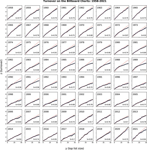
Results of AIC analysis (Table 2) indicate that the neutral model (Equation 4(4) $z=a\ast y^{0.86}$(4) ) can be rejected in favor of the generic model (Equation 3(3) $z=a\ast y^b$(3) ) in all cases, since, for each year between 1958 and 2021, fits obtained with the generic model yielded lower AIC values than those obtained with the neutral model (Akaike weights ranged from ω = 0.974 to 0.999). Figure 3 depicts the average turnover profile on the Billboard Hot 100 Chart over the 1958–2021 period, split by year.

Table 2. Results of AIC Analysis for two competing model fits (generic vs. neutral model) of the Billboard Hot 100 Turnover Profile, by year.

		Generic				Neutral		$\mathrm{\Delta }AIC$
Year	Weeks	$b$	$r^2$	log lik.	AIC	log lik.	AIC
1958	21	.77	.977	34.76	−65.52	25.71	−47.42	18.10
1959	51	.75	.998	80.72	−157.45	33.76	−63.52	93.93
1960	51	.74	.995	68.54	−133.09	30.10	−56.20	76.89
1961	51	.75	.996	72.81	−141.62	32.68	−61.36	80.26
1962	51	.75	.997	76.29	−148.59	35.38	−66.76	81.82
1963	51	.73	.998	89.00	−173.99	28.29	−52.58	121.41
1964	51	.75	.996	73.00	−142.00	33.64	−63.28	78.72
1965	51	.74	.991	56.26	−108.51	28.90	−53.80	54.72
1966	52	.70	.994	66.44	−128.88	20.37	−36.73	92.15
1967	51	.79	.998	82.24	−160.48	48.73	−93.47	67.02
1968	51	.76	.998	85.78	−167.56	39.89	−75.78	91.78
1969	51	.71	.994	66.00	−128.00	23.20	−42.40	85.60
1970	51	.69	.998	89.58	−175.17	18.24	−32.47	142.70
1971	51	.71	.998	88.50	−173.00	23.75	−43.49	129.50
1972	52	.67	.998	90.40	−176.79	15.41	−26.83	149.97
1973	51	.60	.992	65.97	−127.95	2.28	−0.55	127.39
1974	51	.57	.993	70.68	−137.37	−2.06	8.12	145.48
1975	51	.58	.993	69.41	−134.83	−0.80	5.61	140.44
1976	51	.61	.993	67.70	−131.40	3.25	−2.50	128.91
1977	52	.59	.986	55.68	−107.36	−0.25	4.49	111.85
1978	51	.70	.992	59.93	−115.86	19.43	−34.86	81.00
1979	51	.68	.984	47.64	−91.29	13.46	−22.91	68.38
1980	51	.74	.997	75.20	−146.40	31.95	−59.90	86.50
1981	51	.69	.996	74.74	−145.48	19.73	−35.46	110.02
1982	51	.78	.992	56.78	−109.56	39.42	−74.84	34.72
1983	52	.69	.995	69.20	−134.41	18.20	−32.41	102.00
1984	51	.67	.997	83.81	−163.62	15.58	−27.16	136.46
1985	51	.58	.997	89.90	−175.80	−0.59	5.17	180.97
1986	51	.55	.998	93.88	−183.76	−4.07	12.15	195.91
1987	51	.56	.995	77.41	−150.81	−3.59	11.19	162.00
1988	52	.50	.994	79.46	−154.91	−10.04	24.09	179.00
1989	51	.52	.991	69.56	−135.12	−8.05	20.10	155.22
1990	51	.56	.992	70.31	−136.62	−3.74	11.48	148.10
1991	51	.58	.996	80.56	−157.12	−0.30	4.60	161.72
1992	51	.68	.993	62.32	−120.64	16.31	−28.62	92.02
1993	51	.77	.997	77.42	−150.83	40.57	−77.13	73.70
1994	52	.72	.992	59.76	−115.52	23.43	−42.86	72.66
1995	51	.69	.994	67.57	−131.14	17.28	−30.57	100.57
1996	51	.72	.987	48.46	−92.93	22.55	−41.10	51.83
1997	51	.73	.990	54.11	−104.22	26.29	−48.58	55.65
1998	51	.64	.993	66.23	−128.46	8.78	−13.56	114.89
1999	51	.68	.996	76.88	−149.76	17.30	−30.61	119.15
2000	52	.59	.972	41.44	−78.87	−0.81	5.62	84.48
2001	51	.66	.990	56.86	−109.73	11.36	−18.72	91.01
2002	51	.78	.995	63.63	−123.25	43.02	−82.04	41.22
2003	51	.68	.972	35.48	−66.97	11.18	−18.36	48.61
2004	51	.72	.992	58.42	−112.84	23.52	−43.05	69.80
2005	52	.77	.988	47.81	−91.62	33.25	−62.50	29.12
2006	51	.63	.984	50.27	−96.54	6.28	−8.56	87.97
2007	51	.65	.989	56.52	−109.04	10.20	−16.39	92.64
2008	51	.69	.987	50.36	−96.73	15.81	−27.63	69.10
2009	51	.74	.993	62.01	−120.02	28.33	−52.66	67.36
2010	51	.70	.976	37.31	−70.62	15.18	−26.36	44.26
2011	52	.76	.983	41.10	−78.20	26.33	−48.67	29.54
2012	51	.70	.995	67.89	−131.77	20.92	−37.83	93.94
2013	51	.78	.993	59.70	−115.40	39.79	−75.59	39.81
2014	51	.80	.995	66.11	−128.22	49.11	−94.23	33.99
2015	51	.74	.993	60.28	−116.55	30.17	−56.35	60.21
2016	52	.81	.990	49.64	−95.28	42.46	−80.92	14.36
2017	51	.70	.985	47.38	−90.77	17.95	−31.90	58.87
2018	52	.83	.995	60.91	−117.82	57.27	−110.54	7.29
2019	51	.69	.981	42.43	−80.86	14.70	−25.39	55.46
2020	51	.73	.976	36.54	−69.09	18.75	−33.5	35.59
2021	16	.64	.979	43.94	−83.87	6.29	−8.59	75.29

Table 2. Table 2 describes the results of AIC Analysis for two competing model fits (generic vs. neutral model) of the Billboard Hot 100 Turnover Profile, by year. Models are fit against turnover profile averaged across all chart weeks for each of the specified years on the Billboard Hot 100. For all model fits, the number estimated parameters is 2. The Akaike weight (ω) for the generic model is ω = 0.974 in 2018 and exceeds ω > 0.999 in all other years. The generic model is to be preferred over the neutral model in all cases. Weights omitted from table for clarity.

Figure 3. Figure 3 depicts a graph of graphs containing 1958–2021 Billboard Hot 100 Chart turnover profiles, split by year. Each figure reports turnover (z) over the size of the Top Chart (y), averaged across all available weeks in the given year (upper left). Black dots are data. Blue solid line indicates the best-fit predictions according to Equation 3(3) $z=a\ast y^b$(3) (b value located in bottom right). Red-dashed line depicts the best-fit predictions according to neutral model (i.e., Equation 4(4) $z=a\ast y^{0.86}$(4) ; b = 0.86) .

We gain from this analysis a few key pieces of information. First, we obtain a high degree confidence in the feasibility of using Equation 3(3) $z=a\ast y^b$(3) to accurately describe observed turnover profiles. In all cases, observed turnover rates are more accurately described by the generic model (Equation 3(3) $z=a\ast y^b$(3) ) than the neutral model (Equation 4(4) $z=a\ast y^{0.86}$(4) ). In addition, predicted turnover values obtained via Equation 3(3) $z=a\ast y^b$(3) very closely match observed data patterns. This is reflected in the high $r^2$ values (Table 2) and can be seen directly in Figure 3 (blue line). This in turn gives us confidence in the use of the b value derived from Equation 3(3) $z=a\ast y^b$(3) . This is important, because, as was partially mentioned above, the overall shape of the turnover profile generated via Equation 3(3) $z=a\ast y^b$(3) is dictated entirely by the b value. In summary, we have now determined the generic model (Equation 3(3) $z=a\ast y^b$(3) ) can be used to accurately characterize empirical turnover data, with the b value determining the shape of the turnover profile curve.

2.2. Dependent variable: Billboard Hot 100 turnover profiles (1958-2021)

Figure 4 plots the results of the above procedures as a time series (Figure 4). Since the goal of the present investigation is to characterize the likelihood of demand side mechanisms given the turnover observed on the Billboard Hot 100 Charts over time, this time series functions as the dependent in the models and analyses that follow.

Figure 4. Figure 4 plots b values obtained for turnover profiles observed on the Billboard Hot 100 Chart from 1958–2021. Note that all b values are lower than neutral model expectations (dashed line) .

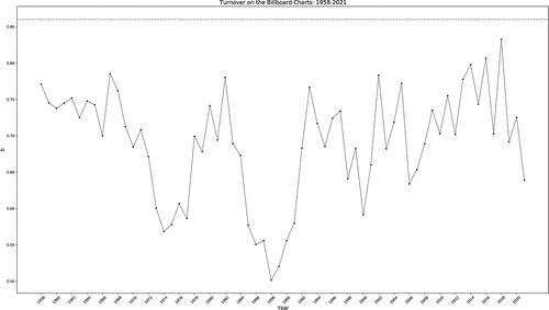
Notice that, in all cases, the values of the exponent b (Mean = .69; SD = 0.08; N = 64) obtained from Billboard Hot 100 turnover profiles are lower than the expected value of 0.86 (Table 2). It was determined via AIC analysis (Table 2) that observed turnover deviates from the amount of turnover we would have observed if the underlying population selected music via a completely random (i.e., which is to say, completely unbiased) copying process. Since the shape of turnover profiles with low b values are concave (Figure 3), this indicates that the most popular songs are consistently changing faster than less popular songs for the whole period from 1958 to 2021. Combined, these results suggest the existence of some type of selection pressure acting to increase the turnover rate of the most popular songs relative to other chart positions.

This effect can be seen more directly by examining changes in the turnover rate (i.e., z/y) over time (Lieberson, 2000). This is accomplished in Figure 5, which plots the turnover rate observed on Billboard Hot 100 $\mathrm{T}\mathrm{o}{\mathrm{p}}_{\mathrm{y}}$Charts from 1958 to 2021 for y = {10, 40, 100}.

Figure 5. Figure 5 plots the turnover rate observed on Billboard Hot 100 $\mathrm{T}\mathrm{o}{\mathrm{p}}_{\mathrm{y}}$Charts from 1958–2021 for y = {10, 40, 100}, along with 95% confidence intervals.

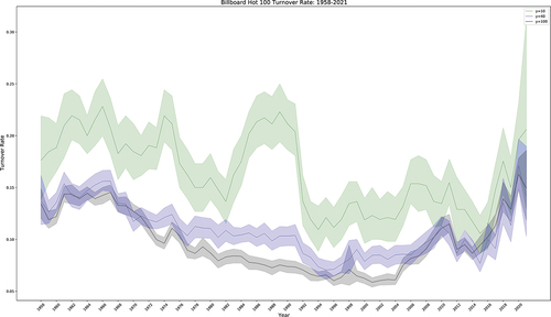
Songs in the Top₁₀ turnover faster than do songs in the Top₄₀ or Top₁₀₀ chart, and this overall trend remains consistently the case over the full 1958–2021 period. However, the turnover rate observed in the Top₁₀ fluctuates dramatically over time and follows a different trend than turnover in the Top₄₀ or Top₁₀₀ charts. Figure 5 additionally enables us to more readily discern the fact that most of the change occurring over time is happening at the top of the charts. Notice for instance, that the turnover rate observed in the Top₁₀ (Figure 5) mirrors the pattern of b results (Figure 4); as b decreases, the Top₁₀ turnover rate increases and overall turnover profiles become more concave (Figure 3). The two periods between 1973 and 1977 and 1985–1991 are particularly interesting. During this period of time, b values are the lowest obtained over the full 1958–2021 period, and a distinct “bend” can be discerned in the shape of turnover profiles at approximately y = 10. This existence of this downward bend suggests that the turnover of songs in the Top₁₀ may have been influenced by process separate from songs located elsewhere on the chart. This possibility is reinforced by the fact that the turnover rate of songs in the Top₁₀ appears to follow a completely separate pattern than the rest of chart during the period of time in question (Figure 5). The turnover rate of songs in the Top₁₀ diverges most sharply from the rest of the chart in 1974 and 1988.

Conversely, years with highest b values (e.g., 1982 and 2018) have more linear turnover profile shapes and begin to approach neutral model expectations (Figure 3). This indicates that the turnover rate of the Top₁₀ is approximately similar to the turnover occurring across the rest of the chart and can be seen in Figure 5 with overlapping 95% confidence intervals.

2.3. Models

The neutral model assumes that individual music selection is entirely a function of random imitation. This is clearly not an accurate description of actual music selection behavior, but it does provide a very useful null hypothesis. In particular, now that we know the extent to which observed data deviates from the predictions of this null model, we can also begin exploring alternative models of music selection by adding theoretically aligned biases to the neutral model and then exploring how these biases impact the shape of the turnover profiles produced. I focus in particular on biases such as status- and network-position, given the evidence that such biases appear to often be prevalent in actual instances of music selection (Bourdieu, 1984; Goldberg, 2011; Mark, 1998; Peterson & Kern, 1996).

I begin by constructing an agent-based model which implements the neutral model of cultural evolution presented in Bentley et al. (2004) and related turnover profile extensions described in (Bentley et al., 2007). Then, I follow prior authors (Acerbi & Bentley, 2014; Mesoudi & Lycett, 2009) and introduce additional models with small modifications designed to capture important aspects of the alternative social transmission mechanisms outlined above. I describe the modeling assumptions used to characterize the transmission mechanisms in the sections below.

2.3.1. Neutral model

I begin by replicating the neutral model of cultural evolution described in Bentley et al. (2004). The model begins with $N$ agents and $N$ songs. Time passes in discrete time steps $\mathrm{t}\in \left\{1,2,..,\mathrm{T}\right\}$. At each time step, all agents simultaneously select a song. With a small probability, $\mu$, an agent introduces a new song to the population. Each of the remaining $\left(1-\mu \right)$N individuals select an agent at random from the previous generation and copy their song choice. At the end of each time step, I record all of the songs present in the population and their frequency, and then rank songs according to observed frequency at time $t$ (i.e., popularity). I then cut this list into 40 $\mathrm{T}\mathrm{o}{\mathrm{p}}_{\mathrm{y}}$ Charts, where the size of the top chart is specified by the variable $y\in \left\{1,2,3,\dots ,40\right\}$. Turnover (z) is defined as the set difference between the $\mathrm{T}\mathrm{o}{\mathrm{p}}_{\mathrm{y}}$ Chart at time t relative to $t-1.$In other words, $z$ records the number of new songs to enter the $\mathrm{T}\mathrm{o}{\mathrm{p}}_{\mathrm{y}}\mathrm{C}\mathrm{h}\mathrm{a}\mathrm{r}\mathrm{t}$ at each time step. The model was run for ($4{\mu }^{-1}+{\mu }^{-1}+50$) total time steps. As Evans and Giometto (2011) note, this gives the model enough time for it to overcome the transient phase of the initial time steps and achieve relative stability ($4{\mu }^{-1}$time steps). After that, turnover will begin fluctuating around a nominal average. Following their recommendations, I allow the model an additional (${\mu }^{-1}+50$ time steps) and then calculate turnover, averaging it on the last (${\mu }^{-1}+50$ time steps). Turnover profiles produced by the neutral model were consistent with those obtained by prior researchers (Acerbi & Bentley, 2014; Bentley et al., 2007; Evans & Giometto, 2011).

In each of the four models outlined below, I add slight modifications to the underlying architecture of the neutral model and “bias” some proportion of agents away from the neutral model and toward one of four alternative models of human decision-making behavior. The specific alterations are outlined in detail for each of the models below.

2.3.2. Song quality

The first alternative model I consider is the song quality model. It is designed to simulate the notion that some songs are intrinsically higher or lower quality than some other songs. The song quality model is implemented as follows. Prior to the model beginning, each song is randomly assigned a level of quality. Song quality is drawn at random from a standard normal distribution ($\mathrm{M}\mathrm{e}\mathrm{a}\mathrm{n}=0,\mathrm{S}\mathrm{D}=1$). In this way, the majority of songs are assigned an intermediate level of quality (i.e., approximately 0), while a few songs will be extremely high/low quality. As was the case in the neutral model, $\left(1-\mu \right)N$ individuals select an agent at random from the previous generation. Here, instead of simply automatically copying their song selection, agents that follow the quality-based selection rule first consider the song’s quality level: if it is higher quality than their current song, they switch; if it is the same or lower, they do not switch songs. A masking parameter, C, determines the proportion of agents that follow the quality-based selection rule. Specifically, at each time step, a total of $C\left(1-\mu \right)N$ agents, on average, are selected at random from the population and marked to follow the quality-based selection rule, while the remaining $\left(1-C\right)\left(1-\mu \right)N$ agents follow the neutral model, and copy the agent’s song without considering its quality. Figure 6 (upper left) depicts turnover profiles produced by the song quality model for various C values, all other parameter values as described previously.

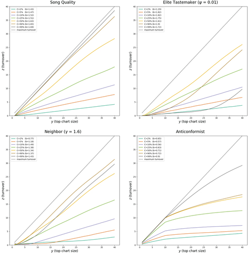
Figure 6. Figure 6 depicts turnover ($z$) over $\mathrm{T}\mathrm{o}{\mathrm{p}}_{\mathrm{y}}$ Charts produced by the song quality (upper left), elite tastemaker ($\psi$=0.01, upper right), neighbor ($\gamma$=1.6, bottom left), and anticonformist (bottom right) models for N = 5000, $\mu =0.01$ for various C values (solid colored lines). Data is averaged across 100 simulation runs for the song quality and anticonformist models, 10 simulation runs for the elite tastemaker model and 20 simulation runs for the neighbor model. $b$ values (each figure, upper left) derive from the best-fit of Equation 3(3) $z=a\ast y^b$(3) for the depicted data at the given parameter values. Maximum turnover (each figure, black dotted line) is equivalent to the curve $z=y$.

2.3.3. Elite tastemaker

The elite tastemaker model incorporates status or class and simulates the idea of a minority social elite leading the tastes expressed by the masses. The model is implemented as follows. First, as was the case in the song quality model, before the model begins each song is randomly assigned a level of quality, with song quality drawn at random from a standard normal distribution ($\mathrm{M}\mathrm{e}\mathrm{a}\mathrm{n}=0,\mathrm{S}\mathrm{D}=1$). Next, a small proportion of agents are randomly assigned “elite” status according to the parameter $\psi$: approximately $\psi$N agents are coded as elite, and the remaining ($1-\psi$)N agents are coded as non-elites. Like the two previous models, at each time step, $\left(1-\mu \right)N$ agents consider a new song. Here however, elite and non-elite agents behave differently. The $\psi \left(1-\mu \right)N$ elite agents consider a song selected at random from among the full universe of possible songs and consider the song’s quality level: if it is higher quality than the song they currently have selected, they switch; if it is the same or lower quality, they do not switch songs. The $\left(1-\psi \right)\left(1-\mu \right)N$ non-elite agents begin as in the neutral model: that is, they select an agent at random from the previous generation and consider their song. Here, instead of simply copying their song selection, non-elite agents first consider whether or not it is also selected by one of the elites: if it is, they switch; if it is not, they do not switch songs. As before, a masking parameter C determines the proportion of agents that follow the elite tastemaker behavior rules. Figure 6 (upper right) depicts turnover profiles produced by the elite tastemaker model for $\psi =0.01$ (i.e., approximately 1% of agents coded as “elite”) for various C values, all other parameters as defined previously.

2.3.4. Neighbor

The neighbor model simulates a preference for songs selected by socially proximate others. In this model, the neutral model is modified to incorporate an underlying social network structure. Beginning with $N$ agents as before, I generate a Barabási and Albert (1999) scale-free random graph $G=\left(N,g\right)$ where $g\subseteq N^2$ and $ij\in g$ if agent $i$ and agent $j$ are linked. All $ij$ links are referred to as “neighbors.” Each agent $i$ is connected to $k$ total neighbors with probability $p_k$, with probabilities decreasing with increased $k$such that $p_k{k}^{-\gamma }$.² As before, a masking parameter C determines the proportion of agents that follow the neighbor-biased selection rule. At each time step, $C\left(1-\mu \right)$N agents, on average, follow the neighbor model; these agents select a neighbor at random and copy their song choice. The remaining $\left(1-C\right)\left(1-\mu \right)$N agents follow the neutral model; these agents select an agent at random from the population and copy their song choice. Figure 6 (bottom left) depicts turnover profiles produced by the neighbor model for $\gamma =1.6$ (i.e., a graph with degree distribution $p\left(k\right)k^{-1.6}$) for various C values, all other parameter as defined previously.

2.3.5. Anticonformist

The anticonformist model simulates a negative reaction to the most popular songs. In keeping with prior implementations of frequency-dependent selection biases (e.g., Acerbi & Bentley, 2014; Mesoudi & Lycett, 2009), the anticonformist model presented here is implemented by providing agents access to information on the $\mathrm{T}\mathrm{o}{\mathrm{p}}_{10}\mathrm{C}\mathrm{h}\mathrm{a}\mathrm{r}\mathrm{t}$ prior to making song selections. Specifically, the model works as follows. Agents designated to follow the anticonformist model first check the $\mathrm{T}\mathrm{o}{\mathrm{p}}_{10}\mathrm{C}\mathrm{h}\mathrm{a}\mathrm{r}\mathrm{t}$ to see if the song they have selected is one of the Top-10 most-popular songs in the population. If it is not, they keep their current song. If it is, they behave according to the neutral model (i.e., select an agent at random from the population, and copy their song choice). In other words, anticonformist agents get rid of their songs if they are “too popular.” As before, the parameter C determines the proportion of agents designated to follow the anticonformist model. Specifically, a total of $C\left(1-\mu \right)N$ agents, on average, follow the anticonformist model, while the remaining $\left(1-C\right)\left(1-\mu \right)N$ agents follow the neutral model. Figure 6 (bottom right) depicts turnover profiles produced by the anticonformist model for various C values, all other parameter values as defined previously.

3. Model results

Information on model behavior is provided in the supplemental online appendix. Key characteristics are presented below.

3.1. Song quality

The song quality model produces convex turnover profiles in which the top songs change more slowly than all other chart positions. Fitting Equation 3(3) $z=a\ast y^b$(3) to the song quality model yielded b values above those expected from an unbiased random copying process (Mean = 1.60, SD = .09, N = 100), and this is true for all C values considered. In fact, even a tiny minority of individuals in the underlying population behaving as specified in the song quality model is enough for the predictions of this model to deviate substantially deviate from the amount of turnover observed in reality, with the shape of the turnover profile becoming approximately linear (b = 0.99) at 1% and noticeably convex at 2% (b = 1.43) or 3% (b = 1.50), a result that indicates that only 1–2% of agents following the song quality model is enough to substantially impact the overall the shape of its overall turnover profile. Turnover profiles rapidly approach maximum turnover as the proportion of agents participating in quality-based selection increases (Figure 6).

3.2. Elite tastemaker

The elite tastemaker model produces convex turnover profiles fitted with b values greater than those expected from the neutral model (Mean = 1.38, SD = 0.49, N = 4900). Turnover profile shapes are strongly impacted by both the C and the $\psi$ parameter. Figure 6 visualizes expected turnover profiles with 1% of agents assigned elite status and provides a typical example of the C parameter on overall model behavior. Turnover profiles become noticeably convex when approximately 2–5% of agents follow elite tastemaker rules and exhibit a very distinctive upward bend, indicating that the most popular songs are changing much more slowly than songs at lower chart regions. Increasing the C parameter pushes the location of this bend outward toward greater y values.

The $\psi$ parameter impacts the magnitude of these overall patterns. However, somewhat interestingly, the impact of the $\psi$ parameter is not linear; across all C values, the most convex turnover profiles are obtained in populations consisting of between 3% and 7% elites. Turnover profiles become less convex as the proportion of elites in the underlying population increases beyond 7% and become indistinguishable from the neutral model when the proportion of elites exceed 20% of the total population. More substantively, the most popular songs change least often when the underlying population contains between 3% and 7% of elites, regardless of the number of agents paying attention to them. Conversely, when the proportion of elites exceeds 20% of the total population, turnover profiles become indistinguishable from a model of simple random copying. This latter effect might well be expected, since a population composed only of elites (and no elite followers) is similar in many respects to the default behavior of the neutral model.

3.3. Neighbor

Turnover profiles produced by the neighbor model were either indistinguishable from the neutral model or convex. b values followed a bimodal distribution determined by the $\gamma$ parameter. Turnover profiles for $\gamma$ <1.24 were indistinguishable from the neutral model (Mean = 0.83, SD = 0.03, N = 6200); turnover profiles for $\gamma$ >1.24 (b = 1.27, SD = 0.14, N = 8800) are convex and exhibit a clear upward bend, indicating that the most popular songs change very slowly relative to less popular songs. Figure 6 visualizes the impact of the C parameter on the shape of this curve at $\gamma$=1.6 and provides a typical example of overall model behavior. The neighbor model requires approximately 3% of agents to participate before the turnover shape is impacted; thereafter, a distinct upward bend appears. The location of this bend moves closer to the top of chart with increasing C and the uptick occurs more sharply with increasing $\gamma$. Maximum b values are obtained with approximately 10% agent participation. Some exceptions to these general trends can be observed in models with very high C (e.g., C = 97–100%).

3.4. Anticonformist

The anticonformist model produces turnover profiles fitted with $b$ values lower than those produced by the neutral model. Turnover profile shapes are extremely sensitive to the existence of agents exhibiting anticonformist behavior; merely 1% of agents behaving as specified in the anticonformist model is enough to produce a concave turnover profile fitted with a b value of .71. Turnover profiles exhibit a distinct downward bend at y = 10, the location of which is readily explained as a function of how anticonformist behavior was implemented in the model (anticonformist agents reject songs in the $\mathrm{T}\mathrm{o}{\mathrm{p}}_{10}$ Chart). The overall concave shape indicates that the most popular songs are changing faster than less popular songs; the downward bend at y = 10 indicates a higher turnover rate in the $\mathrm{T}\mathrm{o}{\mathrm{p}}_{10}$ than all other chart positions. Figure 6 visualizes the impact of the C parameter. The turnover rate of songs in the $\mathrm{T}\mathrm{o}{\mathrm{p}}_{10}$ increases very rapidly as C increases; turnover in $\mathrm{T}\mathrm{o}{\mathrm{p}}_{\mathrm{y}}$ for y > 10 changes more slowly.

4. Turnover analysis: Billboard Hot 100 charts (1958-2021)

In this section, I focus on using the predictions of the different models to interpret the time series presented above (Figure 4). To help focus this effort, I concentrate analytical attention on chart years in which certain diagnostic features of modeled turnover profiles appear in observed turnover data.

4.1. The SoundScan revolution

A variety of technological innovations and entrepreneurial actions forced Billboard to accept a change in the methodology for compiling the weekly charts in 1991. The entire music industry reorganized itself around this methodology change, and for this reason it is sometimes referred to as the SoundScan Revolution (Anand & Peterson, 2000). Charts with the new methodology appeared for the first time on May 25, 1991. Following the switch to SoundScan methodology, turnover dynamics changed significantly. Armed with the new information contributed by the above models, we can now supplement prior analyses of this interesting period with some additional insights.

The impact of the SoundScan revolution is clearly visible in Hot 100 turnover profiles. For example, the 10 lowest b values are observed prior to the 1991 arrival of SoundScan, and the lowest b values observed over the entire course of the Billboard chart’s 63-year history are found between 1985 and 1990, the five years immediately preceding SoundScan’s arrival. A more substantive interpretation of the low b values observed over this period is readily gleaned by evaluating the turnover rate of the Top₁₀ relative to all other chart positions (Figure 5). In this regard, notice that there are two periods prior to SoundScan that follow similar trends, the first occurring between 1973 and 1977 and the second between 1985 and 1991. The b values obtained over these two periods are the lowest observed over the full 1958–2021 period, and a distinct bend can be discerned in the shape of turnover profiles at approximately y = 10. Within these two periods, b values reach local minimums in 1974 (b = .57) and 1988 (b = .50) (Figure 7). The existence of this downward bend suggests that the turnover of songs in the Top₁₀ may have been influenced by process separate from songs located elsewhere on the chart. This possibility is reinforced by the fact that the turnover rate of songs in the Top₁₀ appears to follow a completely separate pattern than the rest of chart during the period of time in question (Figure 5).

Figure 7. Figure 7 depicts average turnover, z, observed in the Top Chart of size $y$ on the Billboard Hot 100 Chart in 1974 and 1988 (dots) along with predicted values according to the best-fit of Equation 3(3) $z=a\ast y^b$(3) (solid line) and the neutral model (b = 0.86, dashed line) .

Of the four models considered above, only the anticonformist model reproduces the characteristics of turnover profiles observed during these two periods. In fact, the shape of the 1974 turnover profile can be reproduced almost exactly in an anticonformist model in which 5% of the underlying population rejects songs in the Top₁₀, and all others copy the music selections of other people at random. Anticonformist models with 11% bias reproduce turnover profiles observed in 1987 and 1990 (b = .56) and come the closest to approximating the turnover profiles of 1988 (b = .50) and 1989 (b = .52), though these extremely low b values were below those produced in any turnover simulations. Since the success of musicians is known to have involved at least some amount of industry-side manipulation, particularly during the period immediately preceding the 1991 SoundScan revolution, the notion that consumption dynamics over this same period of time are best characterized by a model in which sizable minorities of the underlying population are systematically rejecting the industry’s proffered music fare is not altogether far-fetched. This possibility is reinforced by the fact that the distinctive turnover dynamics found only at the very top of the chart disappear completely in 1992, immediately after the methodology change has occurred (Figure 5).

4.2. Digital era: quality searches and long tail effects

The vast majority of all music, book, and movie sales occur within a very small range of total product offerings (Brynjolfsson et al., 2011). Although popularity distributions in the music industry have traditionally been dominated by the superstar effect (Rosen, 1981), this became somewhat less true in digital environments as a result of diminishing search-costs and so-called “long-tail” effects (Anderson, 2008). In short, the long tail theory states that demand and production is increasingly shifting away from the selection and marketing of a small number of best-selling products toward a greater number of niche products in the tail. Just as the superstar effect can explain the phenomenon of long-lasting hit songs as a result of artificially concentrated consumption patterns, the long-tail effect can explain the phenomenon of an increasing number of hit songs as a result of individuals performing more effective or more wide-ranging song quality searches over a less restricted market. There are a variety of indicators of long-tail effects in the digital music era, stemming from a variety of interrelated effects related to reduced search costs, access to online music files, and improved consumer information (Brynjolfsson et al., 2011; Gopal et al., 2006; Hendricks & Sorensen, 2009). A growing body of evidence suggests similar long-tail effects following the arrival of music streaming platforms (Datta et al., 2018; Im et al., 2019). Most relevantly, reducing search cost increases expected turnover (Bhattacharjee et al., 2007; Brynjolfsson et al., 2011; Gopal et al., 2006). The song quality model captures important aspects of the search-related long-tail effect, and the model implemented here similarly predicts rapidly increasing turnover across all chart positions as the proportion of successful song quality searchers in the underlying population is increased. The song quality model is broadly consistent with overall turnover trends and is suggestive of its influence. For example, the overall turnover rate has increased very substantially since 2004 (Figure 5). Spotify became widely available to United States subscribers in 2011, and, shortly thereafter, overall turnover rates increased very dramatically. In 2018, the overall turnover rate reached a level not previously seen since the 1960s, and in 2020 the overall turnover rate on the Hot 100 chart exceeded any point in its entire 63-year history.

4.3. Promotion and network effects

New information made available by the revised chart ranking methodology introduced in 1991 triggered additional industry changes soon thereafter. Of particular note in this regard was the realization that albums exhibited strongest sales immediately following their initial release, which led industry executives to concentrate marketing efforts before rather than after an album’s release (Anand & Peterson, 2000). Since music industry marketing executives have the explicit goal of encouraging others to adopt their music choices, it is possible to examine the effectiveness of various music marketing regimes by searching for diagnostic signatures of the elite tastemaker model in observed turnover profiles. Turnover profiles produced by the elite tastemaker model have a characteristic upward bend, whereby turnover is depressed well below neutral model expectations over multiple top chart positions and then increases dramatically at lower chart positions. As might be expected, a similar effect also occurs in turnover profiles produced by the network model, though the upward bend is generally more subdued for most $\gamma$ values. Although the underlying behavior of the population is different in the two models, it is not surprising that the two models express themselves in similar ways, since the neighbor model is essentially providing a more generalized form of the elite tastemaker model. Indeed, the neighbor model can be made to produce almost identical effects to the elite tastemaker model by moving the $\gamma$ parameter toward higher values, since this has the effect of concentrating the distribution of all network ties into a very small set of extremely well-connected agents.

The exact location of the upward bend depends on various parameter combinations, but in both models it is most directly impacted by C. In the case of the elite tastemaker model, the C parameter directly refers to the proportion of the underlying population adopting the song selections of tastemaking “elites.” Increasing the C parameter results causes the songs selected by tastemakers to remain at the top of the charts for longer periods of time and pushes the location of this bend outward, toward lower chart positions. Conversely, decreasing the C parameter reduces the proportion of agents following the decisions of tastemakers and pushes the location of this bend closer to the top of the chart. As a result, observed turnover profiles exhibiting a clearly discernible upward bend potentially suggest a reduction in the effectiveness of professional song promoters.

Using this information as a diagnostic criterion, I search for Hot 100 turnover profiles with a sudden uptick in turnover at lower chart positions. The single clearest example of this effect occurs in 2020, though faint traces of possibly similar effects can also be discerned in certain earlier chart years (1983, 2004, 2016).

Further considering the very unusual 2020 turnover dynamics, if indeed this uptick effect is telling us something about disrupted promotion, we might also use the results of the neighbor model to further examine the potential mechanisms involved. In the case of the neighbor model, something akin to the 2020 effect can be made to occur by increasing the C parameter, or, in other words, by reducing the likelihood of random information exchange and increasing the role of more localized, strong-tie network effects.

5. Discussion

It was demonstrated above that the simple generic function provided by Acerbi and Bentley (2014) (Equation 3(3) $z=a\ast y^b$(3) ) can be used to characterize the turnover of popular songs on the Billboard Hot 100 charts over the period from 1958 to 2021. Building on prior work involving the neutral model, I began by comparing observed turnover profiles with the turnover profiles we would have observed if music selection in the underlying population consisted of an unbiased random-copying process. Data analysis focused on turnover profile shapes and centered on the value of the exponent b. Observed turnover profiles have overall concave shapes (Figure 3), capturing the higher turnover rate observed in the Top 10 relative to other chart positions and are best fit with an exponent b lower than would be expected under conditions of an unbiased random-copying process (Table 2). Thus, one of the key takeaways of this analysis is that the most popular songs have consistently been changing faster than would be expected from an unbiased selection process over the full 1958–2021 period. This result suggests the existence of selection pressures in the underlying population acting to increase the turnover rate of the most popular songs relative to other chart positions.

Next, using the unbiased neutral model as a baseline, I then investigated departures from this model in order to characterize the likelihood of alternative individual music taste transmission mechanisms in the underlying population. In each of four separate models (song-quality, elite tastemaker, neighbor, anticonformist), I introduced small biases to the neutral model of cultural transmission and then examined the impact of these biases on the shape of turnover profiles produced across a wide variety of parameter combinations. Then, I characterized the likelihood of these four transmission mechanisms by examining the extent to which the models were able to reproduce the diagnostic features of the empirical turnover profiles collected from the Billboard Hot 100 charts over time.

At the broadest level, the models can be usefully contrasted with one another in terms of their predictions concerning turnover at the top of the charts. The song quality, elite-tastemaker, and neighbor models (for $\gamma$ >1.24) yield turnover profiles with an overall convex shape, b values greater than those expected from an unbiased random copying process, and predict rapidly increasing turnover as we move down the chart. As a result, the existence of any of these three selection mechanisms in the underlying population acts to depress the turnover rate in the most popular songs relative to other chart positions. Only the anticonformist model proved capable of reproducing the concave turnover profiles and low b values observed in empirical turnover data.

Although key aspects of each of the four models can be discerned in the turnover data over time, the fact that empirical turnover profiles remained most consistent with anticonformist model expectations over the full 63 year history of the Billboard Hot 100 chart may suggest the presence of similar individual-level biases in the underlying population, with some minority of United States music consumers similarly biased against the consumption of the most popular songs. This result is somewhat surprising. Prior work has demonstrated a fairly consistent bias toward the selection of the most popular items in empirical turnover rates over time, with, e.g., Lieberson (2000) arguing in favor of the existence of something akin to a generalized popularity preference driving individual consumption choices. Additionally, experimental work has demonstrated the existence of a significant “preference for the popular” in individual music selection (Salganik et al., 2006). The results of this prior work led us to believe that we ought to find evidence of a fairly consistent bias toward the selection of the most popular songs in empirical turnover rates over time. However, I find no such evidence of a generalized “preference for the popular” here. In fact, the shape of observed turnover profiles appear to suggest precisely the opposite conclusion: i.e., individuals engaged in the active avoidance of the most popular songs, rather than seeking them out. If indeed there is such a wide-ranging popularity preference, there is no evidence to this effect in the observed data. It could be, however, that a “preference for the popular” does exist but is somewhat more complicated in its effect. For instance, individuals may prefer songs at some level of popularity, but reject songs that have become “too” popular. Something akin to this effect has been pursued elsewhere (e.g., Mesoudi & Lycett, 2009), but has not been specifically connected to turnover profile shapes. The anticonformist model may also provide a plausible explanation for the puzzling data patterns reported by Salganik and Watts (2008), in which the previously reported popularity-based selection mechanisms (Salganik, 2006), were not able to account for the substantial amount of turnover observed in the most-popular songs over time; indeed, to that end, the two authors also note that significant minorities of individuals appeared to demonstrate anticonformist music-selection behavior. Population level turnover patterns reported here are consistent with this hypothesis. Taken together, the two results seem to suggest that individual music consumption is perhaps better modeled not as a preference for popularity, but instead as a simple model of random “drift,” with some small proportion of individuals rejecting popular songs.

With regard to the “bend” sometimes observed in the shape of turnover profiles, I find that this bend is a clearly identifiable data pattern, appearing in both modeled (anticonformist, elite tastemaker, neighbor) and empirical turnover data (Figure 7; Figure 8). This finding suggests that the bend effect is neither a coding artifact (since it appears in empirical data), nor is it always indicative of frequency-dependent individual selection (since it appears in both the neighbor and elite tastemaker models, which do not involve frequency-dependent selection), as had previously been supposed (Acerbi & Bentley, 2014). The bend effect is therefore interesting and can be used to meaningfully distinguish between various selection processes in the underlying population.

Figure 8. Figure 8 depicts average turnover, z, observed in the Top Chart of size $y$ on the Billboard Hot 100 Chart in 1983, 2004, 2016, and 2020 (dots) along with predicted values according to the best-fit of Equation 3(3) $z=a\ast y^b$(3) (solid line) and the neutral model (b = 0.86, dashed line) .

The existence of distinct bends in observed turnover data suggests the existence of two distinct selection mechanisms, the first applying to the selection of the most popular songs and a second process applying to all other songs. It is worth noting, for instance, that the turnover we observe in the Top 40 positions of the Hot 100 chart only very rarely exceeds neutral model expectations for nearly the entirety of its 63-year history. In the few instances where this does occur (2020 being the most obvious example), this occurs only at later chart positions. While the song quality, elite-tastemaker, and neighbor models each depress the turnover rate below neutral model expectations at the top of the chart, only in the elite-tastemaker and neighbor model is the turnover rate depressed across multiple chart positions before suddenly spiking upwards. That this behavior is sometimes observed is rather suggestive. Specifically, in years where a bend upwards occurs is consistent with a lessening role of marketing or promotion activities (elite tastemaker) or, more generally, a disruption in underlying communication networks (neighbor).

With regard to the neighbor model, one of the more interesting results is that the neighbor model produced turnover profiles indistinguishable from neutral model predictions for all social networks with $\gamma$ < 1.28, and produced convex turnover profiles for $\gamma$ >1.28. At a general level these effects are in line with intuition. In less hierarchical social networks ($\gamma$ <1.28, i.e., social networks in which all agents have approximately the same number of friends, all agents have an equal chance of picking the hits. As might be expected, song popularity and turnover in such networks is essentially random, and cannot be distinguished from a completely unbiased cultural drift process. As we increase the $\gamma$ parameter, the social network becomes more hierarchical (i.e., degree distributions become more unequal, with a decreasing proportion of total agents receiving an increasing proportion of all edges). This effectively concentrates decision making power in the hands of fewer people and results in the production of convex turnover profiles in which the most popular songs change more slowly than less popular songs. This effect occurs because in more hierarchical social networks ($\gamma$ >1.28), the ability to pick the hits becomes a function of agent-popularity: songs selected by popular agents always become hits while songs selected by unpopular agents rarely do. Since unpopular agents have less ability to voice their opinions, the most popular songs are “challenged” less often. As a result, songs selected by best-connected agents move to the top of the chart quickly and remain there until they select a new song. Overall, this has the effect of compressing turnover at the top of the charts and produces a convex turnover profile, in which the most popular songs change more slowly than less popular songs.

The network model provides an interesting sociological complement to the neutral model. In particular, another way to think about the neutral model is to imagine it as modeling the transmission of information across a social network consisting exclusively of weak ties, with information being passed only through acquaintances rather than directly connected friends or peers. In such a network, social transmission might be thought of as occurring essentially at random, exactly as the neutral model stipulates. Conversely, if the transmission of information occurs exclusively though directly connected agents, we might think of that type of model as one in which information is transmitted only through strong ties. As a result, the C parameter serves a somewhat unique role in the case of the neighbor model, as it may usefully be thought of as the proportion of strong ties.

Some of the results of the neighbor model are more interesting when considered from this perspective. For instance, in less hierarchical social networks ($\gamma$ <1.28), turnover is apparently completely unaffected by tie strength. Indeed, whether information is received through strong or weak ties, there is no discernible impact on overall song turnover until the degree distribution of the overall social network exceeds a $\gamma$ value of 1.28. However, in more hierarchical networks ($\gamma$ >1.28), the strength of ties begins to matter a great deal. At a broad level, the general pattern of results is as might be expected: as we increase the proportion of agents relying on information received through strong ties (i.e., C), we are increasing the role of friendship networks and thus concentrating decision making power into the people with the most friends. Unsurprisingly, this reduces the amount of turnover we observe in the most popular songs. Zooming in a bit, I find interesting deviations from this general pattern. For instance, the most convex turnover profiles are consistently produced in social networks in which 10% of agents receive information from strong ties and 90% receive information from weak ties (see supplemental online appendix, Figure A11). There are also interesting effects as we remove weak ties entirely. Perhaps as we might expect given prior theory (Granovetter, 1973; Onnela et al., 2007),^, turnover profile shapes change very dramatically as we begin to approach a network in which information is passed only through strong ties (i.e., as C parameter approaches 1.0). To put this another way, I find that allowing even a small amount of random information exchange is enough to substantially alter the shape of the population level turnover profile, reminiscent of a small world effect (Watts & Strogatz, 1998). This is interesting in relation to the positioning of the bend observed in turnover profiles produced by the neighbor model. In particular, increasing the proportion of information passed through strong ties even slightly (i.e., increasing C) rapidly pushes the bend closer to the top of the chart; conversely, increasing the role of weak ties (i.e., decreasing C) pushes the bend farther out and depresses overall turnover across more total chart positions.

The fact that none of these effects are observable until the $\gamma$ parameter crosses the $\gamma$=1.28 threshold was unexpected. While it is perhaps somewhat more possible in the case of the network model that this effect is somehow related to network size (N, see supplemental online appendix B for related discussion), approximately similar $\gamma$ thresholds occur for different N, and it therefore seems more likely that this effect is related to the difficulty of passing messages across networks without clear hubs or other information transmitters (Albert et al., 2000). Future work might make progress in this area by exploring the relationship between turnover and measures of network characteristics related to the difficulty of message passing (e.g., span, average path distance, closeness, etc.). Pursuing this direction would be useful in that it would enable us to characterize turnover in terms of network centrality measures rather than in terms of $\gamma$ values, making the results more intuitive and directly applicable to any number of social network structures.

In this paper, an attempt was made to infer, from aggregated, macro-level turnover data, the likelihood of various conceptions of individual consumption behavior. While the present analysis is set in the context of music consumption, these techniques might easily be applied elsewhere. Indeed, a variety of work has investigated departures from the neutral model (see Shennan, 2011 for a review). However, this analysis is, so far as the present author is aware, the first to link this work to social transmission mechanisms related to network structure or status, known to be relevant in actual instances of music selection (Bourdieu, 1984; Goldberg, 2011; Mark, 1998; Peterson & Kern, 1996). The results presented here document the results of an initial investigation and were necessarily somewhat descriptive. Even so, we learn a variety of things by this method of analysis that were less easily detectable in prior methods, and which may open the way for future research. While we are not able to definitively identify biases operating at an individual level, this analysis has shown that it is possible to make informed inferences about individual level consumption behavior using information from aggregated population level turnover data. Overall, this study contributes to ongoing debates regarding the transmission of taste and the mechanics of fashion change.

Supplemental data

Supplemental data for this article can be accessed on the publisher’s website.

Notes

¹ A power-law popularity distribution means that the vast majority of items are unpopular, and a small minority of items are many, many times more popular than the majority.

² While any number of stochastic graph generators might be employed for this purpose (e.g., Erdos-Renyi, small-world [Watts & Strogatz, 1998]; hierarchical [Clauset et al., 2008], etc.), the Barabási and Albert (1999) scale-free random graph has a variety of characteristics that make its use desirable here. In particular, power-law degree distributions are a common feature in many real-world networks (Albert & Barabási, 2002), the resulting degree distribution is intuitive and can be manipulated directly via the $\gamma$ parameter, it minimizes the number of isolates, and it is computationally efficient.

References

- Acerbi, A., & Bentley, R. A. (2014). Biases in cultural transmission shape the turnover of popular traits. Evolution and Human Behavior, 35(3), 228–236. https://doi.org/10.1016/j.evolhumbehav.2014.02.003
- Albert, R., & Barabási, A.-L. (2002). Statistical mechanics of complex networks. Reviews of Modern Physics, 74(1), 47. https://doi.org/10.1103/RevModPhys.74.47
- Albert, R., Jeong, H., & Barabási, A.-L. (2000). Error and attack tolerance of complex networks. Nature, 406(6794), 378–382. https://doi.org/10.1038/35019019
- Anand, N., & Peterson, R. A. (2000). When market information constitutes fields: Sensemaking of markets in the commercial music industry. Organization Science, 11(3), 270–284. https://doi.org/10.1287/orsc.11.3.270.12502
- Anderson, C. (2008). The long tail: Why the future of business is selling less of more. Hachette Books.
- Barabási, A.-L., & Albert, R. (1999). Emergence of scaling in random networks. Science, 286(5439), 509–512. https://doi.org/10.1126/science.286.5439.509
- Bentley, R. A. (2008). Random drift versus selection in academic vocabulary: An evolutionary analysis of published keywords. PloS One, 3(8), e3057. https://doi.org/10.1371/journal.pone.0003057
- Bentley, R. A., Hahn, M. W., & Shennan, S. J. (2004). Random drift and culture change. Proceedings of the Royal Society of London B: Biological Sciences, 271(1547), 1443–1450. https://doi.org/10.1098/rspb.2004.2746
- Bentley, R. A., Lipo, C. P., Herzog, H. A., & Hahn, M. W. (2007). Regular rates of popular culture change reflect random copying. Evolution and Human Behavior, 28(3), 151–158. https://doi.org/10.1016/j.evolhumbehav.2006.10.002
- Bhattacharjee, S., Gopal, R. D., Lertwachara, K., Marsden, J. R., & Telang, R. (2007). The effect of digital sharing technologies on music markets: A survival analysis of albums on ranking charts. Management Science, 53(9), 1359–1374. https://doi.org/10.1287/mnsc.1070.0699
- Bourdieu, P. (1984). Distinction: A social critique of the judgment of taste. Harvard University Press.
- Boyd, R., & Richerson, P. J. (2005). The origin and evolution of cultures. Oxford University Press.
- Brynjolfsson, E., Hu, Y., & Simester, D. (2011). Goodbye pareto principle, hello long tail: The effect of search costs on the concentration of product sales. Management Science, 57(8), 1373–1386. https://doi.org/10.1287/mnsc.1110.1371
- Bryson, B. (1996). “Anything but heavy metal”: Symbolic exclusion and musical dislikes. American Sociological Review, 61(5), 884–899. https://doi.org/10.2307/2096459
- Burnham, K. P., & Anderson, D. R. (1998). Practical use of the information-theoretic approach. In Model selection and inference (pp. 75–117). New York, NY: Springer. https://doi.org/10.1007/978-1-4757-2917-7_3.
- Cavalli-Sforza, L., & Feldman, M. W. (1973). Models for cultural inheritance I. Group mean and within group variation. Theoretical Population Biology, 4(1), 42–55. https://doi.org/10.1016/0040-5809(73)90005-1
- Cavalli-Sforza, L. L., & Feldman, M. W. (1981). Cultural transmission and evolution: A quantitative approach. Princeton University Press.
- Clauset, A., Moore, C., & Newman, M. E. (2008). Hierarchical structure and the prediction of missing links in networks. Nature, 453(7191), 98–101. https://doi.org/10.1038/nature06830
- Crow, J. K., & Kimura, M. (1997). M. (1970) An Introduction To Population Genetics Theory. Harper and Row.
- Datta, H., Knox, G., & Bronnenberg, B. J. (2018). Changing their tune: How consumers’ adoption of online streaming affects music consumption and discovery. Marketing Science, 37(1), 5–21. https://doi.org/10.1287/mksc.2017.1051
- Evans, T. S., & Giometto, A. (2011). Turnover rate of popularity charts in neutral models. ArXiv preprint. ArXiv:1105.4044. https://arxiv.org/abs/1105.4044
- Goldberg, A. (2011). Mapping shared understandings using relational class analysis: The case of the cultural omnivore reexamined. American Journal of Sociology, 116(5), 1397–1436. https://doi.org/10.1086/657976
- Gopal, R. D., Bhattacharjee, S., & Sanders, G. L. (2006). Do artists benefit from online music sharing?. The Journal of Business, 79(3), 1503–1533. https://doi.org/10.1086/500683
- Granovetter, M. (1973). The strength of weak ties. American Journal of Sociology, 78(6), 1360–1380. https://doi.org/10.1086/225469
- Haampland, O. (2017). Power laws and market shares: Cumulative advantage and the Billboard Hot 100. Journal of New Music Research, 46(4), 356–380. https://doi.org/10.1080/09298215.2017.1358285
- Hahn, M. W., & Bentley, R. A. (2003). Drift as a mechanism for cultural change: An example from baby names. Proceedings of the Royal Society of London B: Biological Sciences, 270(Suppl 1), S120–S123. https://doi.org/10.1098/rsbl.2003.0045
- Harrison, J. R., & Carroll, G. R. (1991). Keeping the faith: A model of cultural transmission in formal organizations. Administrative Science Quarterly, 36(4), 552–582. https://doi.org/10.2307/2393274
- Hendricks, K., & Sorensen, A. (2009). Information and the skewness of music sales. Journal of Political Economy, 117(2), 324–369. https://doi.org/10.1086/599283
- Henrich, J., & Broesch, J. (2011). On the nature of cultural transmission networks: Evidence from fijian villages for adaptive learning biases. Philosophical Transactions of the Royal Society B: Biological Sciences, 366(1567), 1139–1148. https://doi.org/10.1098/rstb.2010.0323
- Herzog, H. A., Bentley, R. A., & Hahn, M. W. (2004). Random drift and large shifts in popularity of dog breeds. Proceedings of the Royal Society of London B: Biological Sciences, 271(Suppl 5), S353–S356. https://doi.org/10.1098/rsbl.2004.0185
- Hesbacher, P., Downing, R., & Berger, D. G. (1975). Sound recording popularity charts: A useful tool for music research: I. Why and how they are compiled. Popular Music & Society, 4(1), 3–18. https://doi.org/10.1080/03007767508591066
- Im, H., Song, H., & Jung, J. (2019). The effect of streaming services on the concentration of digital music consumption. Information Technology & People, 33(1), 160–179. https://doi.org/10.1108/ITP-12-2017-0420
- Kandler, A., & Shennan, S. (2013). A non-equilibrium neutral model for analysing cultural change. Journal of Theoretical Biology, 330, 18–25. https://doi.org/10.1016/j.jtbi.2013.03.006
- Kimura, M. (2020). The neutral theory and molecular evolution. In My thoughts on biological evolution (pp. 119–138). Singapore: Springer. https://doi.org/10.1007/978-981-15-6165-8_8
- Klein, C. C., & Slonaker, S. W. (2010). Chart turnover and sales in the recorded music industry: 1990–2005. Review of Industrial Organization, 36(4), 351–372. https://doi.org/10.1007/s11151-010-9250-z
- Kreitman, M. (1996). The neutral theory is dead. long live the neutral theory. Bioessays, 18(8), 678–683. https://doi.org/10.1002/bies.950180812
- Lieberson, S. (2000). A matter of taste: How names, fashions, and culture change. Yale University Press.
- Manski, C. F. (1993). Identification of endogenous social effects: The reflection problem. The Review of Economic Studies, 60(3), 531–542. https://doi.org/10.2307/2298123
- Mark, N. (1998). Birds of a feather sing together. Social Forces, 77(2), 453–485. https://doi.org/10.2307/3005535
- Merton, R. K. (1948). The self-fulfilling prophecy. The Antioch Review, 8(2), 193–210. https://doi.org/10.2307/4609267
- Mesoudi, A., & Lycett, S. J. (2009). Random copying, frequency-dependent copying and culture change. Evolution and Human Behavior, 30(1), 41–48. https://doi.org/10.1016/j.evolhumbehav.2008.07.005
- Neiman, F. D. (1995). Stylistic variation in evolutionary perspective: Inferences from decorative diversity and interassemblage distance in illinois woodland ceramic assemblages. American Antiquity, 60(1), 7–36. https://doi.org/10.2307/282074
- Obukhova, E., Zuckerman, E. W., & Zhang, J. (2014). When politics froze fashion: The effect of the cultural revolution on naming in beijing. American Journal of Sociology, 120(2), 555–583. https://doi.org/10.1086/678318
- Onnela, J.-P., Saramäki, J., Hyvönen, J., Szabó, G., Lazer, D., Kaski, K., Kertész, J., & Barabási, A.-L. (2007). Structure and tie strengths in mobile communication networks. Proceedings of the National Academy of Sciences, 104(18), 7332–7336. https://doi.org/10.1073/pnas.0610245104
- Peterson, R. A., & Kern, R. M. (1996). Changing highbrow taste: From snob to omnivore. American Sociological Review, 61(5), 900–907. https://doi.org/10.2307/2096460
- Rosen, S. (1981). The economics of superstars. The American Economic Review, 71(5), 845–858. https://www.jstor.org/stable/1803469
- Salganik, M. J., Dodds, P.S., & Watts, D.J. (2006). Experimental study of inequality and unpredictability in an artificial cultural market. Science, 311(5762), 854–856. https://doi.org/10.1126/science.1121066
- Salganik, M. J., & Watts, D. J. (2008). Leading the herd astray: An experimental study of self-fulfilling prophecies in an artificial cultural market. Social Psychology Quarterly, 71(4), 338–355. https://doi.org/10.1177/019027250807100404
- Shennan, S. (2011). Descent with modification and the archaeological record. Philosophical Transactions of the Royal Society of London B: Biological Sciences, 366(1567), 1070–1079. https://doi.org/10.1098/rstb.2010.0380
- Simkin, M. V., & Roychowdhury, V. P. (2003). Copied citations create renowned papers? In ArXiv preprint cond-Mat/0305150. https://arxiv.org/abs/cond-mat/0305150
- Wagenmakers, E.-J., & Farrell, S. (2004). AIC model selection using akaike weights. Psychonomic Bulletin & Review, 11(1), 192–196. https://doi.org/10.3758/BF03206482
- Watts, D. J., & Strogatz, S. H. (1998). Collective dynamics of ‘small-world’networks. Nature, 393(6684), 440–442. https://doi.org/10.1038/30918