Convergence analysis of coarse mesh finite difference method applied to two-group three-dimensional neutron diffusion problem

Abstract

This article presents the convergence analysis of the coarse mesh finite difference (CMFD) method applied to two-group (2-G) three-dimensional (3D) neutron diffusion problem. Two CMFD algorithms are examined: one-node (1-N) CMFD and two-node (2-N) CMFD. Two test problems are used for the study of the convergence behavior: a model problem of homogeneous 2-G 3D eigenvalue problem and the NEACRP LWR transient benchmark problem. The convergence rates of the 1-N and 2-N CMFD algorithms are numerically measured in terms of the convergence of current correction factors (CCFs). The numerical test results are presented as well as the comparison with the previous analytical study. Overall, 1-N CMFD with the CCF relaxation shows a comparable performance to 2-N CMFD for the realistic 3D rod ejection transients.

Keywords:

• convergence analysis
• CMFD
• current correction factor
• eigenvalue problem
• NEACRP
• transient problem

1. Introduction

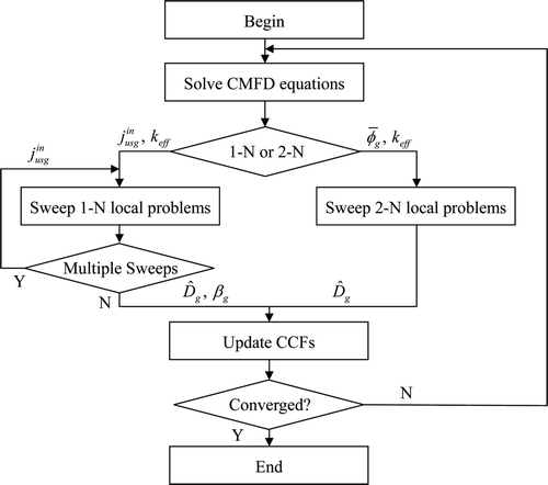
The nonlinear coarse mesh finite difference (CMFD) method uses global/local iterations to converge solutions which were connected by the current correction factors (CCFs) to preserve the interface neutron currents between neighboring nodes. Depending on the local kernel, there are two CMFD methods: one-node (1-N) CMFD and two-node (2-N) CMFD. The advantage of 1-N CMFD is a simpler implementation and the possibility of the direct 2-G CMFD formulation for multi-group (MG) problems, and the disadvantage is the fact that additional spatial sweeps are needed to make the convergence behavior more stable [1–4]. The advantage of 2-N CMFD is a stable convergence, and the disadvantage is the difficulty in applying the method to hexagonal lattice and the lack of applicability to direct 2-G CMFD for MG problems [1,4].

Depending on the situation, one method can be preferred to the other method. Sometimes both methods can be applied. In order to make a wise choice, we need to understand the convergence characteristics of the two methods. Once we know the exact (or converged) value of CCFs, then the solution can be obtained in one iteration with those CCFs. Therefore, the convergence of CCFs in the global/local update is the key element of the convergence analysis of CMFD methods, and this article focuses on the convergence rates of the CCFs.

The nonlinear CMFD algorithm [5] has been widely used for the acceleration of both diffusion and transport calculations [6–9]. For the acceleration of transport calculation, Cho and Park performed analytic studies on the convergence characteristics of CMFD method using Fourier analysis [10]. For the acceleration of diffusion calculation, Lee et al. reported the analytical convergence analysis of CMFD method which was performed by linearizing the nonlinear CMFD algorithm and applying Fourier analysis to the linearized algorithm, which means that their convergence analysis is applicable to the system in the asymptotic convergence region [11–14]. The key results of the previous theoretical analysis can be summarized as follows [13]:

–	One-node CMFD is stable for small mesh size and becomes unstable for large mesh size.
–	The instability of 1-N CMFD can be remedied to become unconditionally stable by introducing optimum under-relaxation and the expression of optimum value has been analytically derived.
–	Two-node CMFD is unconditionally stable regardless of what the mesh sizes are.
–	Overall, 2-N CMFD shows better performance than 1-N CMFD or coarse mesh rebalance.

However, the above analysis was limited to simple model problems, i.e., one-group (1-G) one-dimensional (1D) fixed source problems (FSPs), primarily because of the complexity of the analytic derivation of the spectral radius for MG multidimensional eigenvalue problems (EVPs). Therefore, the convergence studies in this article were performed ‘numerically’ with the ‘practical’ two-group (2-G) three-dimensional (3D) steady state and transient problems.

In this article, the stability/instability of the CMFD algorithms in the asymptotic convergence region is studied as a function of mesh size and relaxation parameter. When partial currents are used for CCF calculations, due to the weak coupling of the nodes, the 1-N CMFD becomes unstable as the mesh size increases. For small mesh size, both 1-N and 2-N CMFD methods are stable. But still even with small mesh sizes, depending on the magnitude of node average flux in the denominator of the CCF calculations, pathological CCFs can be obtained and the CMFD matrix cannot be converged due to the loss of diagonal dominance (or positive definiteness) of CMFD matrices. However, this is not the point of analysis in this article [4]. This aspect of CMFD convergence characteristics was reported elsewhere by Zika and Downar [15].

In Section 2, the nonlinear CMFD methodologies with 1-N and 2-N kernels and how to measure the convergence rates are presented, and the numerical convergence analysis is presented in Section 3. Section 4 concludes this article.

2. Methodology

The 2-G 3D steady state neutron diffusion equation can be written in Cartesian coordinates as:

where φ _g is a scalar flux, D_g is a diffusion coefficient, Σ_rg is a removal cross section, Σ_fg is a fission cross section, g represents the neutron energy group, ν is the average number of neutrons per fission, Σ₁₂ is the scattering cross section, and k _eff is the effective multiplication factor. The conventional transverse integrated nodal methods (TINMs) exploit the transverse integration of Equation (1) which yields a 1D diffusion equation [6]:

where , , and φ _ug (u) is the transverse integrated 1D flux, L_ug (u) is a u-directional transverse leakage, u = x,y,z, g = 1, 2, and D and A are 2 × 2 matrices representing diffusions and absorptions/fissions, respectively. The 1-N and 2-N kernels of CMFD method are presented in the following subsections.

2.1. 1-N kernel

The formulation of 1-N kernel based on the partial current coupling is rarer than the 2-N based kernel in the literatures. Especially, in the 1-N formulation of this article, all directions are coupled simultaneously. Therefore, the formulations are given here in detail. For the 1-N kernel purpose, the general solution of Equation (2) can be written as [6]:

where a_up ; p = 1, 2, 3, 4 ; g = 1, 2; u = x,y,z are six unknown coefficients to be determined per direction, are four coefficients of transverse leakage shape, and

and sn(κu) = sin(κu) or sinh(κu), cn(κu) = cos(κu) or cosh(κu), and are two bucklings, and , shape functions f ₁(ξ) = ξ, f ₂(ξ) = 3ξ² − 1/4, ξ = u/h_u , and h_u is the u-directional mesh size. In the conventional TINMs, the coefficients, s, are determined by node average transverse leakages of the previous iteration. In the 1-N approach of this article, however, they are determined by the solutions of current iteration together with other four coefficients, a_up , and therefore, the solutions to three directions are directly coupled and solved simultaneously. The constraints required to determine the total 18 unknown coefficients are 4 consistency conditions of node average fluxes, 2 nodal balance equations, and 12 incoming partial currents:

•	4 consistency conditions of the node average flux:
•	2 nodal balance equations:
•	12 incoming partial currents: where l and r represent left and right surfaces, respectively. The node average flux consistency conditions and nodal balance equations can be rewritten more compactly as: where ‘NB’ means ‘nodal balance.’ This can be expressed using the coefficients of the general solution as: where , , , and T and W are 6 × 6 matrices.

The incoming partial current conditions also can be rewritten as:

where M _u and P _u are 2 × 2 matrices and

where , B = diag(B _x ,B _y ,B _z ), P = 2 × diag(P _x ,P _y ,P _z ), and B _u and P _u ; u = x,y,z are 2 × 2 matrices.

Rearranging Equations (9) and (11) leads to

Equation (12) is solved for the even coefficients by Gaussian elimination of the 6 × 6 linear system of equations. The coefficients a are obtained from the even coefficients using Equation (13) and the odd coefficients are obtained by Equation (10) for each direction.

In the 1-N CMFD algorithm, two correction factors for each node interface are required and two different forms of the CCFs were considered:

•

Shin's CCF form [7] Two net currents at left and right interfaces of a node are corrected by the correction factors as: where J s, φs; s = l, r are currents and fluxes at left/right surfaces which are calculated from partial currents, , and the CCFs are defined by: and the relaxation of CCFs is defined as: where is the CCF from Equation (15), η is the relaxation parameter, and k is the iteration index.

•

Joo's CCF form [16] Net current and surface flux are corrected by two separate correction factors: where and α = θr/(θr + θl); θ = D/h. Two correction factors are defined as and the under-relaxation is defined by where is the CCF and β(k+1/2) is the surface flux correction factor (SFCF) obtained using Equation (18), η is the relaxation parameter, and k is the iteration index. The two forms of the CCFs are compatible in the sense that one form can be obtained from the other form, i.e., using Shin's CCFs, Equation (15), the net current and surface flux of Joo's form can be obtained as [17]: where

Joo's CCF form is the same as the conventional 2-N CCF in the PARCS code [6]. Therefore, the 1-N CMFD with Joo's form correction factors was implemented using the existing CCFs with additional SFCFs. The 1-N CMFD with Shin's form correction factors was also implemented using the 2-N CCFs and SFCFs after the conversion of Shin's correction factors to Joo's form by Equation (20).

2.2. 2-N kernel

The formulation of the 2-N kernel can be found in many literatures [6]. Only the essence of the method is briefly reviewed here. The constraints to solve 2-N problem are two node average fluxes and two continuity conditions of flux and current at the interface of the two nodes. From the solutions to the 2-N problems, the CCFs can be updated by

where is the interface current from the high-order 2-N nodal solution, is a standard finite difference coupling coefficients, is the CCF, and and represent node average fluxes at left and right nodes, respectively.

2.3. Estimate of convergence rate

The CMFD algorithm is a nonlinear algorithm of global/local iterations which achieves high-order accuracy using the CCFs updated progressively by the solution to local problems. The iteration can be written as below using operator notation:

where two matrices and F represent neutron removals and generations, respectively. Superscript (k) represents iteration index and K_n is either 1-N kernel (n = 1) or 2-N kernel (n = 2). Figure 1 shows the calculation flow of the global/local iterations. The 1-N CMFD can adopt multiple 1-N local sweeps as needed, which are the partial current updates of all nodes with the latest information of partial currents from neighboring nodes.

Figure 1. Flowchart of CMFD global–local iteration.

The convergence of CCFs can be measured using the formula:

The CCFs in each iteration can be written as

where is the exact CCFs and ε^(k) is the error in the CCFs at iteration k. By inserting Equation (25) into Equation (24), the convergence rate can be rewritten as:

where is the error reduction factor in each iteration.

In order to obtain a consistent numerical measurement of the convergence rate of CCFs, the iterations to solve Equation (2) between CCF updates are fully converged. However, the usual practice is to employ only three or four outer iterations between CCF updates in order to reduce the overall computational time. It is worthwhile to note that the convergence rate of Equation (24) is not like the dominance ratio of EVP, i.e., the dominance ratio is essentially dependent on the core size measured in diffusion length, but literally the convergence rate of CCFs is a function of the mesh size.

3. Convergence analysis

The convergence analysis was performed in two steps. The first step is to examine the general convergence behavior depending on various parameters using a simple geometry model problem, a cube. The behavior of numerically measured convergence rate was discussed with comparison to that of analytic study in the literature [11–14]. The second step is to examine the convergence of CMFD in a more realistic problem, the NEACRP benchmark [18].

3.1. Simple 2-G 3D problem

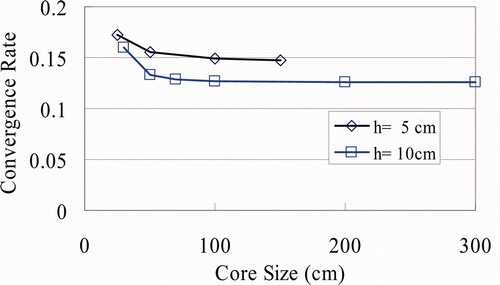
The first 2-G 3D model problem is an EVP of which the geometry is a cube with uniform meshes in all directions. The material is homogeneous with the cross section data given in Table 1, which were taken from NEACRP LWR transient benchmark. The ‘incoming current zero' boundary conditions are used at all boundaries. As indicated in Figure 2, the convergence rate of the CCFs becomes asymptotic for the core size greater than 100 cm. Test cases are listed in Table 2. The core sizes for each test case are greater than 100 cm and the number of total meshes in each direction is chosen to be greater than or equal to 10. It was noted that the measured convergence rates become asymptotic after three to four global–local iterations, and the values of convergence rates in Figures 2 – 7 are the asymptotic values of each case.

Figure 2. Sensitivity of convergence rate to core size (2-N CMFD; 2-G 3D model EVP).

Figure 3. Convergence rate vs. mesh size (2-N CMFD; 2-G 3D model problem).

Figure 4. Sensitivity of 1-N CMFD convergence rate to mesh size and relaxation parameter with 2-G 3D model EVP (Shin's CCF; Jacobi-style Jin update, single sweep). (a) Convergence rate vs. mesh size and (b) convergence rate vs. relaxation parameter.

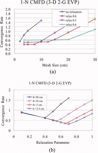
Figure 5. Sensitivity of 1-N CMFD convergence rate to sweep strategy for the 2-G 3D model EVP (Shin's CCF).

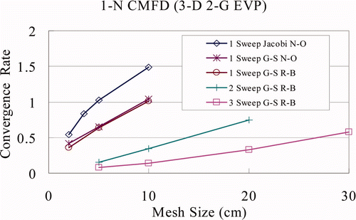
Figure 6. Sensitivity of 1-N CMFD convergence rate to CCF form (Jacobi/G–S-style double sweeps, R–B ordering).

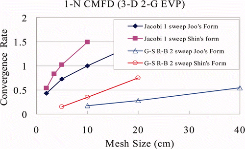
Figure 7. Sensitivity of 1-N CMFD convergence rate to CCF form (Shin's form B: CCF update after all the local 1-N sweeps).

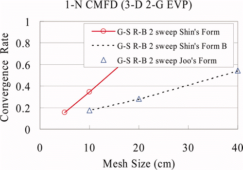
Table 1. Cross section data for 2-G problem.

Group g	Dg	Σrg	νΣfg	Σ12
1	1.500711	0.026968	0.00498277	0.0182498
2	0.415038	0.065255	0.0839026

Table 2. List of test cases (3D cubic core with uniform meshes).

# of meshes	Mesh size (cm)	Core size (cm)
50	2	100
30	3.5	105
20	5	100
14	7.5	105
10	10	100
10	20	200
10	40	400
10	80	800

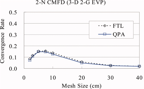
In Figure 3, the convergence rate of the CCFs vs. mesh size is plotted for 2-N CMFD algorithm. The FTL and QPA represent ‘flat transverse leakage’ and ‘quadratic polynomial approximation,’ respectively. The overall trend is the same as that of the 1-G 1D FSP obtained from the theoretical analysis [11,12] regardless of the transverse leakage approximation, i.e., (1) the convergence rates approach zero as the mesh size becomes smaller, (2) the convergence rates get bigger and then become smaller when the mesh size becomes even larger, and (3) the convergence rates are always smaller than unity.

As for the 1-N CMFD algorithm, there are several possible variants depending on the specific strategy used to implement it as in Table 3. In this table, ‘Jacobi Jin update’ denotes the partial current update strategy such that all the incoming currents of 1-N problem are provided from CMFD, and the ‘Gauss–Seidel (G–S) Jin update’ means if updated outgoing partial currents of the adjacent node are available, then they will be used as incoming currents of the node of interest instead of the ones from the CMFD. Therefore, in the natural ordering ‘G–S Jin update’ scheme, half of the incoming currents of a node are from the adjacent nodes and the other half are from the CMFD.

Table 3. Parameters for 1-N CMFD strategy.

Parameter	Value
CCF form	Shin's form/Joo's form
Jin update	Jacobi/G–S
# of sweeps	1–7
Under-relaxation	0 <  η  < 1
Sweep ordering	Natural/red–black

Shin's CCF with a single 1-N sweep (Jacobi-style Jin update) was used for a sensitivity study of the 1-N CMFD convergence rate to mesh sizes and relaxation parameters. The results shown in Figure 4 reveal the following trends:

•	As the mesh size increases, the convergence becomes slower and eventually the algorithm diverges (convergence rate >1.0) for large mesh size.
•	An under-relaxation can expand the stability domain of the algorithm. The more the under-relaxation, the larger becomes the stability domain.
•	As the mesh size approaches zero, the convergence rate approaches (1−η) when the under-relaxation of  η  is applied, which is consistent with the fact that the finite difference method solutions approach the exact solutions as the mesh size goes to zero [13].

The above observations and the trends of the convergence behavior shown in Figure 4 are the same as those of the 1-G 1D FSP model problem theoretically analyzed in [10]. The different convergence behaviors of the CCFs in the 1-N and 2-N CMFDs (for large mesh size, the 1-N CMFD diverges whereas the 2-N CMFD converges) can be attributed to the nature of local problems. The solutions to the 2-N local problems are tightly coupled, in other words, the high-order nodal current term in Equation (21) is calculated from the analytic expression of the fluxes over the two nodes. However, the current terms in Equation (15), 1-N CMFD, are mixed with the partial currents from the neighboring nodes which are not necessarily consistent with the analytic solutions of the current node. This inconsistency gets worse as the mesh size becomes bigger which explains the instability of 1-N CMFD for large mesh size.

In Figure 5, the test results of 1-N CMFD are shown with Shin's CCF form and for the 2-G 3D model EVP. The ‘N-O’ and ‘R–B’ represent ‘natural ordering’ and ‘red–black ordering,’ respectively. Based on this figure, the following observations are made:

•	The ‘G–S Jin update’ converges faster than the ‘Jacobi Jin update.’
•	The natural ordering and the red–black ordering show comparable performance which means the effect of sweeping order is small due to the high performance of CMFD.
•	The more sweeps of the 1-N local problems, the faster the convergence.

When evaluating the CCFs of 1-N CMFD, the net currents and surface fluxes are calculated from partial currents. The coupling of neighboring nodes is not as strong as the 2-N CMFD which uses flux and current continuity conditions. In order to achieve the stronger coupling of the nodes in 1-N CMFD formulation, multiple sweeps of partial current updates are needed.

As shown in Figure 6, the 1-N CMFD with Joo's CCF form converges faster than the one with Shin's CCF. However, as discussed earlier with Equation (20), the two CCF forms are equivalent. Then the difference of convergence performance observed in Figure 6 was turned out to be caused by the difference of how the CCFs are updated. Joo's CCFs are updated after the 1-N sweeps for all the nodes are finished since they are dependent on two nodes. Conversely, Shin's CCFs are updated right after each 1-N solution, which is more consistent with the concept of 1-N CMFD. If Shin's CCFs are also updated in the same way as Joo's CCF, then the convergence rates of the two CCFs are same, which is shown in Figure 7 .

3.2. NEACRP LWR transient problem

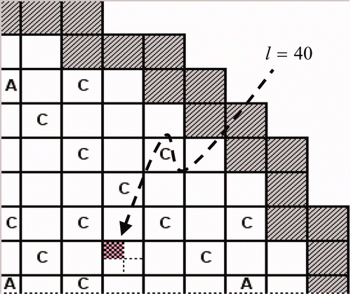
The NEACRP LWR transient benchmark is a well-known 2-G 3D rod ejection transient problem [18] and the quarter-core (QC) geometry is shown in Figure 8. The solutions to this problem obtained using PARCS 1-N kernel are confirmed to be consistent with those from 2-N kernel regardless of the number of 1-N local sweeps. For all cases in this section, the CCFs are updated in every three outer iterations.

Figure 8. PARCS quarter-core model for NEACRP A1 case (A: 100 steps, C: 200 steps).

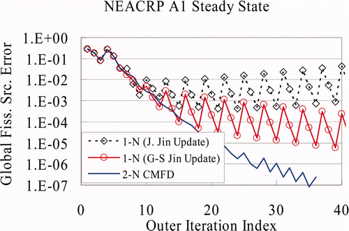
In Figure 9, the ‘Jacobi Jin update’ is compared with the ‘G–S Jin update’ in terms of the global fission source error reduction for the NEACRP A1 steady state problem. The global fission source error is defined as:

where 𝛙 ^(k) = vector of  𝛙 ^m,(k); m ∈ core, is a fission source at node m, and k is an outer iteration index.

Figure 9. Jacobi vs. G–S Jin update (Joo's CCF, triple sweeps).

Joo's CCF and a triple-sweep method were used with the 1-N kernel. As indicated, the ‘Jacobi Jin update’ diverges but the ‘G–S Jin update’ converges. Also, oscillations are observed for the global fission source of the 1-N CMFD algorithm but not for the 2-N CMFD algorithm.

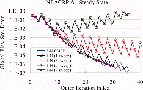
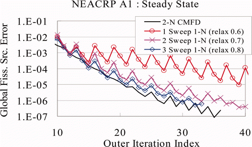
As indicated in Figure 10, a single-sweep 1-N CMFD algorithm diverges because of the oscillations of the fission source error. As the number of 1-N sweeps increases, the oscillations of the global fission source errors are damped out, and with seven sweeps, the oscillations almost disappear and the error reduction of the 1-N CMFD becomes comparable to the one of 2-N CMFD.

In Table 4, for the NEACRP A1 problem, the number of nodal updates and the execution time of PARCS are summarized for 1-N and 2-N CMFDs. Both 1-N and 2-N CMFD use the analytic nodal method as a higher-order nodal method for local problems. ‘Nodal update’ represents the number of CCF updates using the solutions to the local 1-N or 2-N problems, and ‘CMFD update’ represents the number of outer iterations to solve the EVP with CCFs in the steady state and to solve the FSP with CCFs in the transient calculations. As indicated in this table, a five-sweep 1-N CMFD is comparable to a 2-N CMFD in terms of the number of updates, for both steady state and transient calculations. However, the five-sweep 1-N CMFD algorithm takes longer time than 2-N CMFD because of the multiple sweeps. The CMFD execution time of 2-N CMFD and the five-sweep 1-N CMFD is similar to each other but the nodal update time of the five-sweep 1-N CMFD takes much longer.

Table 4. Summary of NEACRP A1 calculation (Joo's CCF, G–S Jin update, R–B ordering).

(a) Steady state
	2-N	1-N (# of sweeps)
		1	3	5	7
Critical Boron Concentration (CBC: ppm)	561.256	Diverge	561.256
Nodal update	13		35	12	10
CMFD update	36		99	35	30
Nodal time (s)	0.7		5.4	2.9	3.3
CMFD time (s)	1.9		4.3	1.9	1.8
Total time (s)	2.6		9.8	4.9	5.2
Time/nodal sweeps (s)	0.053	0.052	0.049	0.047
(b) Transient
	2-N	1-N (# of sweeps)
		3	5	7
Peak power (%)	125.87	125.86	125.84	125.99
Nodal update	31	49	28	24
CMFD update	274	292	278	270
Nodal time (s)	1.7	7.7	6.7	7.9
CMFD time (s)	19.9	20.5	19.6	19.4
Total time (s)	27.9	34.6	32.9	33.6
Time/nodal sweeps (s)	0.054	0.052	0.048	0.047

In Figure 11, various under-relaxation parameters were tested for the single-sweep 1-N CMFD algorithm using the NEACRP A1 steady state problem. As indicated in Figure 11(a), the optimum relaxation appears to be about 0.6. As shown in Figure 11(b), the CCF oscillations can be damped by under-relaxation. The CCF in this figure is from the thermal energy group at the west boundary of the node of axial plane index k = 9, and radial node index l = 40. Since the total number of axial plane is 18, the plane number of k = 9 represents almost the middle of the core and the radial location of l = 40 is shown in Figure 8. In Table 5, the optimum relaxation also seems to be 0.6 in terms of the number of nodal updates and total computation time. As indicated, even the optimized 1-N CMFD algorithm is slower than the 2-N CMFD.

Figure 10. Convergence rate of 1-N/2-N CMFD (Joo's CCF, G–S Jin update).

Figure 11. Convergence of single-sweep 1-N CMFD for NEACRP A1 steady state (Joo's CCF, G–S Jin update, R–B ordering). (a) Error reduction vs. relaxation parameter and (b) CCF convergence of node (k = 9, l = 40).

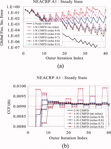
Table 5. Summary of NEACRP A1 steady state with single-sweep 1-N CMFD (Joo's CCF, G–S Jin update, R–B ordering).

	2-N	1-N (relaxation parameter)
		1.0–0.8	0.7	0.6	0.5
CBC (ppm)	561.256	Diverge	561.256
Nodal update	13		89	28	33
CMFD update	36		251	79	91
Nodal time (s)	0.7		6.42	2	2.3
CMFD time (s)	1.9		10.23	3.8	4.1
Total time (s)	2.6		16.7	5.9	6.5
Time/nodal sweeps (s)	0.053		0.072	0.072	0.070

The same tests were performed with double 1-N sweeps. As indicated in Table 6, the optimum value of relaxation is about 0.7, and the 1-N CMFD algorithm is comparable to the 2-N CMFD algorithm in terms of the number of nodal updates, but not in terms of the computation time. Again, the same tests were performed for triple local 1-N sweeps. The performance of the 1-N CMFD algorithm with triple 1-N sweeps and with a relaxation parameter of 0.8 is comparable to the 2-N CMFD in terms of the number of updates as indicated in Table 7.

Table 6. Summary of NEACRP A1 steady state with double-sweep 1-N CMFD (Joo's CCF, G–S Jin update, R–B ordering).

	2-N	1-N (relaxation parameter)
		1	0.9	0.8	0.7	0.6
CBC (ppm)	561.256	Diverge	561.256
Nodal update	13		80	23	14	16
CMFD update	36		226	65	40	46
Nodal time (s)	0.7		9.19	2.7	1.6	1.9
CMFD time (s)	1.9		10.58	3.3	2.4	2.5
Total time (s)	2.6		19.83	6.1	4.1	4.5
Time/nodal sweeps (s)	0.053		0.057	0.058	0.056	0.060

Table 7. Summary of NEACRP A1 steady state with triple-sweep 1-N CMFD (Joo's CCF, G–S Jin update, R–B ordering).

	2-N	1-N (relaxation parameter)
		1	0.9	0.8	0.7
CBC (ppm)	561.256	561.256
Nodal update	13	35	17	11	12
CMFD update	36	99	49	33	35
Nodal time (s)	0.7	5.4	2.6	1.7	1.9
CMFD time (s)	1.9	4.3	2.3	1.8	1.9
Total time (s)	2.6	9.8	4.9	3.6	3.8
Time/nodal sweeps (s)	0.053	0.052	0.050	0.052	0.052

In Figure 12, the 1-N CMFD algorithms with single, double, and triple 1-N sweeps are plotted with optimum relaxation parameter of each case. In terms of convergence rate (global fission source error reduction), the triple-sweep 1-N CMFD algorithm with a relaxation parameter of 0.8 shows the best performance.

Figure 12. Convergence of 1-N CMFD for NEACRP A1 steady state (Joo's CCF, G–S Jin update, R–B ordering).

As shown in Tables 8 and 9, the triple-sweep 1-N CMFD algorithm with a relaxation parameter of 0.8 was tested for NEACRP steady state and transient calculations. In terms of the number of CCF updates, the 1-N CMFD algorithm is comparable to the 2-N CMFD algorithm for both the steady state and transient problems. However, the computation time takes longer for the 1-N CMFD algorithm because of the multiple 1-N sweeps. This can be mitigated by further optimizations of the 1-N kernel coding. As indicated in these tables, the 1-N kernel has more potential for optimization.

Table 8. Summary of NEACRP steady state calculations (Joo's CCF; triple sweeps (1-N CMFD), G–S Jin update, R–B ordering, under-relaxation 0.8).

	A1		B1		C1		A2
	HZP, QC		HZP, QC		HZP, HC		HFP, QC
Parameters	2-N	1-N	2-N	1-N	2-N	1-N	2-N	1-N
Nodal update	13	11	11	11	11	19	13	11
CMFD update	36	33	31	32	31	58	37	33
Nodal time (s)	0.7	1.9	0.6	1.7	1.3	5.8	0.8	1.7
Total time (s)	2.8	3.8	2.4	3.8	4.9	12.1	3.5	4.1
Time/nodal sweep (s)	0.055	0.056	0.055	0.052	0.115	0.102	0.058	0.052

Table 9. Summary of NEACRP transient calculations (Joo's CCF; triple sweeps (1-N CMFD), G–S Jin update, R–B ordering, under-relaxation 0.8).

	A1		B1		C1		A2
	HZP, QC		HZP, QC		HZP, HC		HFP, QC
Parameters	2-N	1-N	2-N	1-N	2-N	1-N	2-N	1-N
Peak power (%)	125.9	126.0	125.9	126.0	482.2	482.4	108.6	108.6
Nodal update	31	29	30	28	19	15	10	10
CMFD update	274	277	262	261	327	322	182	208
Nodal time (s)	1.7	4.3	1.8	4.3	2.3	4.5	0.6	1.5
Total time (s)	27.9	29.7	27.3	29.5	81.3	83.3	19.1	20.1
Time/nodal sweep (s)	0.054	0.050	0.060	0.051	0.120	0.101	0.056	0.050

4. Conclusion

The 1-N CMFD and 2-N CMFD have their own strengths and weaknesses; The 1-N CMFD is unstable for large mesh size and its performance is at best just comparable to 2-N CMFD with multiple sweeps and by applying the optimum relaxation parameters, but the 1-N local solution can update neutron energy spectrum by itself such that a direct 2-G CMFD is applicable to MG problems.

The convergence characteristics of 1-N and 2-N CMFD algorithms were studied by numerical estimate of convergence rates with two test problems: a 2-G 3D (cube) EVP and the NEACRP LWR transient benchmark problem. The NEACRP benchmark is very close to realistic commercial LWRs. It was observed that the overall trends of the CCF convergence behavior are similar to those of the simple 1-G 1D FSPs analyzed in [13] by Fourier analysis applied to the linearized algorithms. Specifically,

•	The convergence rate of CCFs depends on the mesh size and the relaxation parameters.
•	The 2-N CMFD algorithm is always stable. However, the 1-N CMFD algorithm is stable only for small mesh sizes and diverges for large mesh sizes.
•	With under-relaxation of the CCFs, the stability domain of 1-N CMFD algorithm can be substantially expanded.
•	The larger the mesh size is, the more under-relaxation is required to stabilize.

Additional insights about the algorithms obtained from the numerical tests can be summarized as follows, which might be useful for the practical implementation of the 1-N CMFD algorithm:

•	As the number of local 1-N sweeps increases, the CCFs converge faster.
•	The ‘G–S Jin update’ is more effective than the ‘Jacobi Jin update’ as expected.
•	The CCF update after sweeping all nodes is more efficient than the instantaneous CCF updates right after solving each 1-N problem.

The previous analytical convergence study was done for FSPs [11–13]. The detail numerical investigation of convergence rates in this article as a function of parameters has been performed for EVPs and transient problems. The transient problem consists of multiple FSPs. The study in this article shows that the insights obtained from analytical study for 1-G 1D FSPs can be applied to 2-G 3D EVPs and also transient problems, and not much difference in the performances was observed between EVPs and transient problems. Currently, a theoretical convergence analysis for EVPs is just starting and the results will be reported later. The evaluation of the multiplication factor in the EVPs introduces another level of nonlinearity into the algorithm, which makes the analysis more difficult, but it appears that it can be treated like other nonlinearities in the analysis, i.e., by linearization and applying Fourier analysis.

Acknowledgements

This work was supported by National Research Foundation of Korea grant funded by the Korea Government (Ministry of Education, Science and Technology).

References

- Yoon , J.I. and Joo , H.G. 2008 . Two-level coarse mesh finite difference formulation with multigroup source expansion nodal kernels . J. Nucl. Sci. Technol , 45 : 668 – 682 .
- Yamamoto , A. , Endo , T. , Tabuchi , M. , Sugimura , N. , Ushio , T. , Mori , M. , Tatsumi , M. and Ohoka , Y. 2010 . AEGIS: an advanced lattice physics code for light water reactor analyses . Nucl. Eng. Technol , 42 : 500 – 519 .
- Shim , C.B. , Jung , Y.S. , Yoon , J.I. and Joo , H.G. 2011 . Application of backward differentiation formula to spatial reactor kinetics calculation with adaptive time step control . Nucl. Eng. Technol , 43 : 531 – 546 .
- Chao , Y.A. 2000 . Coarse Mesh Finite Difference Methods and Applications . PHYSOR 2000 . May 7–12 2000 .
- Smith , K.S. 1983 . Nodal method storage reduction by non-linear iteration . Trans. Am. Nucl. Soc , 44 : 265
- Joo , H.G. , Barber , D.A. , Jiang , G. and Downar , T.J. 1998 . PARCS: a multi-dimensional two-group reactor kinetics code based on the nonlinear analytic nodal method , Purdue University . PU/NE-98-26
- Shin , H.C. , Kim , Y.H. and Kim , Y.B. 1999 . One-node coarse-mesh finite difference algorithm for fine-mesh finite difference operator . Trans. Am. Nucl. Soc , 81 : 150
- Smith , K.S. and Rhodes , J.D. III . 2002 . Full-Core, 2-D, LWR Core Calculations with CASMO-4E . Proc. ANS Reactor Physics Topical Meeting, PHYSOR 2002 . October 7–10 2002 . [CD-ROM]
- Joo , H.G. , Cho , J.Y. , Kim , H.Y. , Zee , S.Q. and Chang , M.H. 2002 . Dynamic Implementation of the Equivalence Theory in the Heterogeneous Whole Core Transport Calculation . Proc. ANS Reactor Physics Topical Meeting, PHYSOR 2002 . October 7–10 2002 . [CD-ROM]
- Cho , N.Z. and Park , C.J. 2003 . A Comparison of Coarse Mesh Rebalance and Coarse Mesh Finite Difference Accelerations for the Neutron Transport Calculations . Nuclear Mathematical and Computational Sciences: A Century in Review, American Nuclear Society . April 6–11 2003 . [CD-ROM]
- Lee , D. , Downar , T.J. and Kim , Y. 2003 . Convergence Analysis of the Nonlinear Coarse Mesh Finite Difference Method . Nuclear Mathematical and Computational Sciences: A Century in Review, American Nuclear Society . April 6–11 2003 . [CD-ROM]
- Lee , D. 2003 . Convergence analysis of the coarse mesh finite difference method , West Lafayette , IN : School of Nuclear Engineering, Purdue University . Ph.D. thesis
- Lee , D. , Downar , T.J. and Kim , Y. 2004 . Convergence analysis of the coarse mesh finite difference method for one-dimensional fixed source neutron diffusion problem . Nucl. Sci. Eng , 147 : 127 – 147 .
- Lee , D. , Downar , T.J. and Kim , Y. 2004 . Numerical Convergence Analysis of the CMFD Method for the Three-Dimensional Two-group Diffusion Problem . PHYSOR2004 . April 25–29 2004 . [CD-ROM]
- Zika , M.R. and Downar , T.J. 1993 . Numerical divergence effects of equivalence theory in the nodal expansion method . Nucl. Sci. Eng , 115 : 219 – 232 .
- Joo , H.G. One-Node Solution Based Nonlinear Analytic Nodal Method . Proc. KNS Spr. Mtg . [CD-ROM].
- Lee , C.-H. 2001 . A multi-level acceleration method for the multi-group SP3 approximation to the neutron transport equation , West Lafayette , IN : School of Nuclear Engineering, Purdue University . Ph.D. thesis
- Finnemann , H. and Galati , A. 1992 . NEACRP 3-D LWR core transient benchmark , Nuclear Energy Agency . NEACRP-L-335 (Rev. 1)