Study on application of kriging to evaluation of radioactivity concentration for ensuring compliance with the criterion of site release

Abstract

In the field of safety regulation systems for the decommissioning of nuclear facilities, a reliable method for ensuring compliance with the criterion of site release is an important technical issue to be resolved in Japan. Considering that kriging can consider the spatial correlation of radioactivity concentrations between different points, we propose a method of applying kriging to ensure compliance with the site release criterion. Estimated radioactivity concentrations exhibit uncertainty, which results in a certain probability of the occurrence of decision errors regarding site release. We describe a method for calculating the uncertainty as a function of the number of measurement points and establish a minimum number of measurement points required for a given error probability. We applied the proposed method and a conventional statistical method to two sample cases. It was observed that the proposed method appropriately estimated the mean radioactivity concentration even if the measurement points were distributed inhomogeneously. This method was observed to lead to an efficient measurement requiring fewer measurement points relative to the conventional statistical method when spatial correlation existed.

Keywords:

• decommissioning
• site release
• kriging
• radioactivity
• uncertainty
• decision error
• measurement

1. Introduction

After a nuclear power plant has ceased the operation permanently, the plant is dismantled and the nuclear site is eventually released from regulatory control. To ensure safety of the nuclear site after site release, the Multi-Agency Radiation Survey and Site Investigation Manual (MARSSIM) [1] was developed in the United States (US), which provides a nationally consistent consensus approach for conducting radiation surveys and investigations at potentially contaminated sites. Several nuclear sites have been released from regulatory control in the US in accordance with the standards dictated by MARSSIM. While a number of nuclear power plants are at a decommissioning stage, in Japan, specific regulatory rules ensuring safe site release have not yet been established. It is therefore one of the important issues in Japan to establish regulations for site release and a procedure of ensuring compliance with the site release criterion. Discussions conducted by the Ministry of Economy, Trade, and Industry regarding confirmation of decommissioning termination including site release began in 2011 [2].

As a component for ensuring compliance with site release criterion, radioactivity concentrations of the soil on the site are measured and evaluated. For effective measurement and evaluation, a sampling method is applied to extract a number of measurement points in a survey unit and a statistical analysis of the measured data is conducted. Here it must be noted that a spatial correlation of radioactivity concentrations generally exists between different measurement points. However, this spatial correlation is not addressed using conventional statistical methods (CSMs) in which the radioactivity concentrations are assumed to be independent and distributed randomly. The method employed in MARSSIM is based on a CSM. On the other hand, kriging [3], originally developed in the mining industry, accounts for spatial correlation by introducing a variogram, which is expressed by one-half of the expected squared difference between two data values separated by a distance (see Equation (A.6) in Appendix A). Kriging is therefore expected to more accurately estimate the radioactivity concentration distribution using data obtained from a sampling method, and to better ensure compliance with the site release criterion.

The objective of this study is to propose a method to apply kriging to the evaluation of the mean radioactivity concentration for determination of site release. We address the uncertainty in the estimated mean radioactivity concentration, show a method of calculating the minimum number of measurement points required for a given occurrence probability of decision errors, and apply the method to two sample cases to demonstrate its validity.

2. Postulated procedure for ensuring compliance with release criterion

To ensure public safety after site release, public exposure must be assured to not exceed site release criterion (e.g., regulatory limit in terms of dose or risk). The radioactivity concentration corresponding to the release criterion is called the derived concentration guideline level (DCGL) in MARSSIM, and is defined therein as “the DCGL, based on pathway modeling, is the uniform radioactivity concentration level within a survey unit that corresponds to the release criterion (e.g., regulatory limit in terms of dose or risk)” [1].

However, the radioactivity concentration in a survey unit is generally not distributed uniformly. This condition yields a question as to what is an appropriate statistical quantity of the radioactivity concentration to be compared with the DCGL. We have proposed that the mean of the radioactivity concentration [4] is an appropriate quantity for consistency with the DCGL. We use Equations (1) and (2), referred to as the unity rule, to judge whether a survey unit complies with the site release criterion. (1) $$f\le 1,$$(1) (2) $$f=\sum _k\bar{z}\left(k\right)/d\left(k\right).$$(2)

Here $\bar{z}\left(k\right)$ is the mean concentration of radionuclide k in the survey unit and d(k) is the DCGL for radionuclide k. The mean concentrations $\bar{z}\left(k\right)$ and the quantity f estimated based on values measured at a number of measurement points in the survey unit exhibit uncertainties. The uncertainties originate from several causes. These uncertainties are associated with, for example, (1) a number of measurement points that do not rigorously cover all points in the survey unit, and (2) measured data that inherently include measurement error. We first focus on addressing the uncertainty due to (1), and then discuss considering that due to (2). Uncertainties in the estimation of f result in a certain probability of the occurrence of decision errors in site release. Because the decision error probability depends on the number of measurement points, it is important to obtain a relationship between the decision error probability and the number of measurement points. This relationship has been established for CSMs [1,5], but not for kriging. We therefore discuss the appropriate number of measurement points in a survey unit when kriging is applied.

The overall postulated procedure for ensuring compliance with the release criterion is described in Figure 1, which is the result of a previous study [6]. The procedure begins with a historical site assessment, where the operator investigates the presence or absence of radionuclide leakage or discharge during the period of operation and dismantling of the facility. Areas are then divided into non-impacted and impacted areas. Non-impacted areas are judged to meet the release criterion. Impacted areas are divided into three classes, Classes 1, 2, and 3, based on a classification survey. Areas demonstrating a possibility of f > 1 are assigned Class 1, those where f ⩽ 1 are expected are assigned Class 2, and those where the radioactivity concentration is as low as background level are assigned Class 3.

Figure 1. Schematic of the postulated procedure for ensuring compliance with release criterion in Japan (edited from [6]).

After areas are classified, Class 1 areas are remediated, a remedial action support survey is performed, and then the areas are reclassified as Class 2. Regarding Class 2 or Class 3 areas, a survey unit is assigned, methods of measurement and determination for site release are determined, and then a final status survey is conducted. The final status survey comprises scanning measurements and static measurements. Scanning measurement involves gross γ-ray measurement to locate hot spots. The area over which scanning measurements are conducted is larger for the higher radioactivity concentration class. The static measurement is employed to obtain radioactivity concentration data for determining the survey unit's compliance with the site release criterion. For that purpose, a number of samples are collected and measured by a radiation detector, such as a high-purity germanium detector, to obtain radioactivity concentration.

After the radioactivity concentrations in all survey units are determined to comply with the site release criterion, confirmation by the regulatory body is conducted, and the process of decommissioning is terminated.

The three types of surveys, where measurement and evaluation of radioactivity concentrations are conducted in the above procedure, are given as the classification survey, the remedial action support survey for Class 1 areas, and the final status survey for Class 2 and Class 3 areas. In this study, we specifically address the static measurement conducted in the final status survey and the subsequent decision on whether all survey units comply with the criterion of site release.

3. The relationship between ordinary kriging and mean kriging I

In order to estimate the mean of radioactivity concentration in a survey unit, we apply mean kriging I (MK-I) [7] and mean kriging II (MK-II) [3] which estimate the mean value of a physical quantity on an area-wide basis. In MK-I, the estimation variance of the difference between the estimator of the mean and the true mean is minimized to obtain kriging solutions. Variograms among all points are considered to estimate the mean. On the other hand, in MK-II, the estimation variance of the estimator of the mean is minimized. Variograms among only the measurement points are considered to estimate the mean.

In discussing the number of measurement points required to be given in Section 4, it is needed to establish the relationship between ordinary kriging and MK-I solutions. This section describes the relationship that we have established. The general explanation on kriging including ordinary kriging, MK-I, and MK-II is provided in Appendix A. We refer to some equations in Appendix A in the following discussion.

A variogram model used in MK-I is the same as that in ordinary kriging. Using the solutions, the normalized weighting factor wⁱ_α (see Equations (A.1) and (A.2)), and the Lagrange parameter μⁱ (see Equation (A.7)) of ordinary kriging, we introduce the following quantities given by Equations (3) and (4): (3) $$w_{\alpha }=\frac{1}{N}\sum _{i=1}^N{w}_{\alpha }^i,$$(3) (4) $$\mu =\frac{1}{N}\sum _{i=1}^N{\mu }^i,$$(4) where N is the total number of meshes in the survey unit. Summing all equations in Equation (A.7) from i = 1 to N and dividing the summed quantity by N, we obtain (5) $$\begin{array}{c}\sum _{\beta =1}^n\frac{1}{N}\sum _{i=1}^N{w}_{\beta }^i\gamma ({\mathbf{x}}_{\alpha }-{\mathbf{x}}_{\beta })+\frac{1}{N}\sum _{i=1}^N{\mu }^i\hfill \\ =& \frac{1}{N}\sum _{i=1}^N\gamma ({\mathbf{x}}_{\alpha }-{\mathbf{x}}_i),\hfill \end{array}$$(5) where γ(x_α − x_β) is a variogram between two points x_α and x_β, and n is the number of measurement points. Substituting Equations (3) and (4) into Equation (5), we obtain (6) $$\sum _{\beta =1}^n{w}_{\beta }\gamma ({\mathbf{x}}_{\alpha }-{\mathbf{x}}_{\beta })+\mu =\frac{1}{N}\sum _{i=1}^N\gamma ({\mathbf{x}}_{\alpha }-{\mathbf{x}}_i).$$(6)

Furthermore, we obtain the condition on w_α as (7) $$\begin{array}{c}\hfill \sum _{\alpha =1}^n{w}_{\alpha }=\sum _{\alpha =1}^n\frac{1}{N}\sum _{i=1}^N{w}_{\alpha }^i=\sum _{i=1}^N\frac{1}{N}\sum _{\alpha =1}^n{w}_{\alpha }^i=\sum _{i=1}^N\frac{1}{N}=1.\end{array}$$(7)

Comparing Equations (6) and (7) with Equations (A.20) and (A.18) for MK-I, respectively, we recognize that the introduced quantities, w_α and μ, satisfy the same equation as ${\bar{w}}_{\alpha }$ and $\bar{\mu }$, which indicates that w_α and μ are solutions of MK-I.

Using the MK-I solutions expressed by those of ordinary kriging given by (8) $${\bar{w}}_{\alpha }=\frac{1}{N}\sum _{i=1}^N{w}_{\alpha }^i,$$(8) (9) $$\bar{\mu }=\frac{1}{N}\sum _{i=1}^N{\mu }^i,$$(9) the estimated mean and its standard error are expressed as (10) $${\bar{z}}_n^{*}=\frac{1}{N}\sum _{\alpha =1}^n\sum _{i=1}^N{w}_{\alpha }^{i}z\left({\mathbf{x}}_{\alpha }\right),$$(10) (11) $$\begin{array}{ccc}\hfill {\sigma }_n^2& =& \frac{1}{N}\sum _{i=1}^N{\mu }^i+\frac{1}{N^2}\sum _{\alpha =1}^n\sum _{i=1}^N{w}_{\alpha }^i\sum _{j=1}^N\gamma ({\mathbf{x}}_{\alpha }-{\mathbf{x}}_j)\hfill \\ -\frac{1}{N^2}\sum _{i,j=1}^N\gamma ({\mathbf{x}}_i-{\mathbf{x}}_j).\hfill \end{array}$$(11)

4. Method for application of kriging

4.1. Equation to determine the minimum number of measurement points required

By employing a random variable $\bar{Z}\left(k\right)$ corresponding to $\bar{z}\left(k\right)$, a random variable F corresponding to the quantity f is expressed as (12) $$F=\sum _k\bar{Z}\left(k\right)/d\left(k\right).$$(12)

By replacing $\bar{Z}\left(k\right)$ by ${\bar{Z}}_n^{*}\left(k\right)$ (see Equations (A.14) or (A.22)), F is approximated by (13) $$F_n^{*}=\sum _k{\bar{Z}}_n^{*}\left(k\right)/d\left(k\right),$$(13) and the estimated value f*_n for the random variable F*_n is given by (14) $$f_n^{*}=\sum _k{\bar{z}}_n^{*}\left(k\right)/d\left(k\right),$$(14) where subscript n denotes the number of measurement points. The estimated mean of the radioactivity concentration ${\bar{z}}_n^{*}\left(k\right)$ exhibits uncertainty as expressed in terms of the standard error. The standard error depends on the number of measurement points. As a result, f*_n also exhibits uncertainty depending on the number of measurement points. Two types of errors, denoted as Type I and Type II errors, in decisions regarding the site release are considered. The Type I error determines that the value of f is less than or equal to 1 when the true value is above 1. The Type II error correspondingly determines that the value of f is above 1 when the true value is less than or equal to 1. It is necessary to control error probabilities to make decisions that maintain safety within an intended confidence level. This can be achieved by adjusting the number of measurement points in accordance with the relationship between error probabilities and the number of measurement points. Using statistical hypothesis testing and assuming that the estimated mean value ${\bar{z}}_n^{*}\left(k\right)$ follows a normal distribution, the minimum number of measurement points required to control error probabilities within a chosen range is given by the solution to the following equation [4]: (15) $$f_n^{*}+(k_{\alpha }+k_{\beta }){\sigma }_n\left(f_n^{*}\right)=1$$(15) for given probabilities α and β for Type I and Type II errors, respectively. Here σ_n(f*_n) is a standard error of f*_n for the number of measurement points n, and k_α and k_β are the upper α-point and β-point in the standard normal distributions, respectively. When we address only one objective radionuclide (radionuclide k) to be evaluated, Equation (15) is rewritten as (16) $${\bar{z}}_n^{*}\left(k\right)+(k_{\alpha }+k_{\beta }){\sigma }_n\left(k\right)=d\left(k\right).$$(16)

Because f*_n and ${\bar{z}}_n^{*}\left(k\right)$ are somewhat dependent on n and, as n increases, σ_n(f*_n) and σ_n(k) generally decrease, the left-hand side of Equation (15) or (16) – denoted here as a comparison function – has a tendency to be a decreasing function of n. The minimum number of measurement points required is given by the point of intersection between the curve of the comparison function and the line of y = 1 or y = d(k) in the orthogonal coordinate system with horizontal axis corresponding to n and vertical axis corresponding to the value of the comparison function and y.

4.2. Method to determine the minimum number of measurement points required

To determine the minimum number of measurement points required, it is necessary to express σ_n(f*_n) in Equation (15) as an explicit function of n. Using solutions of MK-I or MK-II, the estimation variance of f*_n or σ_n(f*_n)² is expressed as given by Equations (17)–(20) [4]: (17) $$\begin{array}{c}\hfill {\sigma }_n{\left(f_n^{*}\right)}^2=E\left[{\left(F_n^{*}-E\left[F\right]\right)}^2\right]=\sum _k{\sigma }_n{\left(k\right)}^2/d{\left(k\right)}^2+C\left(f\right)\end{array}$$(17) (18) $$C\left(f\right)=\sum _{\genfrac{}{}{0pt}{}{k,k^{\text{'}}\hfill }{(k\ne k^{\text{'}})\hfill }}\mathrm{Cov}(k,k^{\text{'}})/\left(d\left(k\right)·d\left(k^{\text{'}}\right)\right)$$(18) (19) $$\begin{array}{ccc}\hfill \mathrm{Cov}(k,k^{\text{'}})& =& E[({\bar{Z}}_n^{*}\left(k\right)-E\left[\bar{Z}\left(k\right)\right])·({\bar{Z}}_n^{*}\left(k^{\text{'}}\right)-E\left[\bar{Z}\left(k^{\text{'}}\right)\right])]\hfill \\ =& \sum _{\beta ,{\beta }^{\text{'}}=1}^n{\bar{w}}_{\beta }\left(k\right){\bar{w}}_{{\beta }^{\text{'}}}\left(k^{\text{'}}\right)C_{k{k}^{\text{'}}}({\mathbf{x}}_{{\beta }^{\text{'}}}-{\mathbf{x}}_{\beta })\hfill \end{array}$$(19) (20) $$\begin{array}{c}\hfill C_{k{k}^{\text{'}}}({\mathbf{x}}_{{\beta }^{\text{'}}}-{\mathbf{x}}_{\beta })=E\left[(Z(k,{\mathbf{x}}_{\beta })-\bar{z}\left(k\right))(Z(k^{\text{'}},{\mathbf{x}}_{{\beta }^{\text{'}}})-\bar{z}\left(k^{\text{'}}\right))\right]\end{array}$$(20)

The quantity C(f) expresses the contribution from the correlation of radioactivity concentrations of two radionuclides. The function $C_{k{k}^{\text{'}}}({\mathbf{x}}_{{\beta }^{\text{'}}}-{\mathbf{x}}_{\beta })$ can be calculated by approximating $\bar{z}\left(k\right)$ by ${\bar{z}}_n^{*}\left(k\right)$ and using the measured value for Z(k, x_β), as is the case for the experimental variogram.

In the following subsections, we describe how to express σ_n(k)², given as the first term in Equation (17), as a function of n in MK-I and MK-II.

4.2.1. Mean kriging I

To approximately express the n-dependency of σ_n(k)², we use the ordinary kriging solution and the relationship between ordinary kriging and MK-I, where the fact that ordinary kriging is an exact interpolator plays an essential role. Namely, if the point to be estimated coincides with a measurement point, the estimated value at that point exactly equals to the corresponding measured value, where the weighting factor and the Lagrange parameter at the point x_β are given by (21) $$w_{\alpha }^{\beta }\left(k\right)={\delta }_{\alpha \beta },$$(21) (22) $${\mu }^{\beta }\left(k\right)=0,$$(22) with (23) $${\delta }_{\alpha \beta }=\left\{\begin{array}{ccc}\hfill 1& \hfill \mathrm{for}& \hfill \alpha =\beta \\ \hfill 0& \hfill \mathrm{for}& \hfill \alpha \ne \beta \end{array}.\right.$$(23)

We now record measurement points in x_β(β = 1, 2, …, n), points other than the measurement points in x_s(s = n + 1, n + 2, …, N), and both points in x_i(i = 1, 2, …, N).

Using Equations (A.7), (9), and (22), we rewrite the first term on the right-hand side of Equation (A.21) for the estimation variance as (24) $$\begin{array}{ccc}\hfill \frac{1}{N}\sum _{i=1}^N{\mu }^i\left(k\right)& =& \frac{1}{N}\sum _{s=n+1}^N{\mu }^s\left(k\right)=\frac{1}{N}\sum _{s=n+1}^N{\gamma }_k({\mathbf{x}}_{\alpha }-{\mathbf{x}}_s)\hfill \\ -\frac{1}{N}\sum _{s=n+1}^N\sum _{\beta =1}^n{w}_{\beta }^s\left(k\right){\gamma }_k({\mathbf{x}}_{\alpha }-{\mathbf{x}}_{\beta }).\hfill \end{array}$$(24)

The number of values contributing to the summation for the first and second terms on the right-hand side of Equation (24) are (N − n) and (N − n)(n − 1), respectively, because of the fact that the value of the variogram at the origin is zero, i.e., γ_k(x_α − x_β) = 0 for x_α = x_β. Considering that the mean of w^s_β(k) is 1/n (see Equation (A.8)), we introduce the following averaged quantities for the first and second terms on the right-hand side of Equation (24): (25) $$⟨{\gamma }_{\alpha }\left(k\right)⟩=\frac{1}{N-n}\sum _{s=n+1}^N{\gamma }_k({\mathbf{x}}_{\alpha }-{\mathbf{x}}_s),$$(25) (26) $$\begin{array}{ccc}\hfill ⟨w{\gamma }_{\alpha }\left(k\right)⟩& =& \frac{1}{(N-n)(n-1)}\frac{1}{1/n}\hfill \\ \times \sum _{s=n+1}^N\sum _{\beta =1}^n{w}_{\beta }^s\left(k\right){\gamma }_k({\mathbf{x}}_{\alpha }-{\mathbf{x}}_{\beta }).\hfill \end{array}$$(26)

We then obtain (27) $$\begin{array}{ccc}\hfill \frac{1}{N}\sum _{i=1}^N{\mu }^i\left(k\right)& =& \left(1-\frac{n}{N}\right)\{\frac{1}{n}⟨w{\gamma }_{\alpha }\left(k\right)⟩+⟨{\gamma }_{\alpha }\left(k\right)⟩\hfill \\ -⟨w{\gamma }_{\alpha }\left(k\right)⟩\}.\hfill \end{array}$$(27)

While the quantities ⟨γ_α(k)⟩ and ⟨wγ_α(k)⟩ in Equation (27) depend on the measurement point x_α, Equation (27) does not depend on the measurement point x_α because it originates from μⁱ(k) which does not depend on x_α. To eliminate the dependency of ⟨γ_α(k)⟩ and ⟨wγ_α(k)⟩ on the measurement point x_α, we average ⟨γ_α(k)⟩ and ⟨wγ_α(k)⟩ over all measurement points x_α(α = 1, 2, …, n) and rewrite Equation (27) as given by Equations (28)–(30). (28) $$\frac{1}{N}\sum _{i=1}^N{\mu }^i\left(k\right)=\left(1-\frac{n}{N}\right)\left(\frac{1}{n}{\gamma }_{1w}\left(k\right)+{\gamma }_1\left(k\right)-{\gamma }_{1w}\left(k\right)\right)$$(28) (29) $$\begin{array}{ccc}\hfill {\gamma }_{1w}\left(k\right)& =& \frac{1}{n}\sum _{\alpha =1}^n⟨w{\gamma }_{\alpha }\left(k\right)⟩=\frac{1}{(N-n)(n-1)}\hfill \\ \times \sum _{\alpha =1}^n\sum _{s=n+1}^N\sum _{\beta =1}^n{w}_{\alpha }^s\left(k\right){\gamma }_k({\mathbf{x}}_{\alpha }-{\mathbf{x}}_{\beta })\hfill \end{array}$$(29) (30) $$\begin{array}{c}\hfill {\gamma }_1\left(k\right)=\frac{1}{n}\sum _{\alpha =1}^n⟨{\gamma }_{\alpha }\left(k\right)⟩=\frac{1}{N-n}\frac{1}{n}\sum _{\alpha =1}^n\sum _{s=n+1}^N{\gamma }_k({\mathbf{x}}_{\alpha }-{\mathbf{x}}_s)\end{array}$$(30)

Similarly, the sum of the second and third terms on the right-hand side of Equation (A.21) is rewritten as given by Equations (31)–(33). (31) $$\begin{array}{c}\sum _{\beta =1}^n\frac{1}{N}\sum _{i=1}^N{w}_{\beta }^i\left(k\right)\frac{1}{N}\sum _{j=1}^N{\gamma }_k({\mathbf{x}}_{\beta }-{\mathbf{x}}_j)-\frac{1}{N^2}\sum _{i,j=1}^N{\gamma }_k({\mathbf{x}}_i-{\mathbf{x}}_j)\hfill \\ =-\left(1-\frac{1}{N}\right)\left(1-\frac{n}{N}\right)({\gamma }_2\left(k\right)-{\gamma }_{2w}\left(k\right))\hfill \end{array}$$(31) (32) $${\gamma }_2\left(k\right)=\frac{1}{(N-1)(N-n)}\sum _{s=n+1}^N\sum _{i=1}^N{\gamma }_k({\mathbf{x}}_s-{\mathbf{x}}_j)$$(32) (33) $$\begin{array}{c}\hfill {\gamma }_{2w}\left(k\right)=\frac{1}{(N-1)(N-n)}\sum _{\beta =1}^n\sum _{s=n+1}^N{w}_{\beta }^s\left(k\right)\sum _{i=1}^N{\gamma }_k({\mathbf{x}}_{\beta }-{\mathbf{x}}_i)\end{array}$$(33)

Combining Equations (28)–(33) yields Equations (34) and (35), (34) $${\sigma }_n{\left(k\right)}^2=\left(1-\frac{n}{N}\right)\left(\frac{1}{n}{\gamma }_{1w}\left(k\right)+\gamma \left(k\right)\right)$$(34) (35) $$\begin{array}{c}\hfill \gamma \left(k\right)={\gamma }_1\left(k\right)-{\gamma }_{1w}\left(k\right)-\left(1-\frac{1}{N}\right)({\gamma }_2\left(k\right)-{\gamma }_{2w}\left(k\right))\end{array}$$(35)

It is noted that, as expected, σ_n(k)² is zero for n = N because no uncertainty exists when measurements are executed at all mesh points. It should be recognized that, thus far, σ_n(k)² has been expressed without approximation, and the n-dependence of σ_n(k)² has not been explicitly extracted because – to be exact – the factors γ₁(k), γ_1w(k), γ₂(k), γ_2w(k) are dependent on n. To explicitly express the n-dependency of σ_n(k)², we make the following approximation in calculating those factors. We calculate them using the measured data that include the number of initial measurement points (NIMP) n₀ because the quantities are averaged values and their n-dependency is considered to be weak. Hence, the n-dependency of σ_n(k)² is approximately expressed in the form of Equation (34) with γ_1w(k) and γ(k) being constant.

Substituting Equations (17) and (34) into Equation (15) and approximating f*_n by the value calculated using n₀ measured data, we obtain a quadratic equation reflecting the value of n given by (36) $$\begin{array}{c}\sum _k\left(1-\frac{n}{N}\right)\left\{\frac{1}{n}{\gamma }_{1w}\left(k\right)+\gamma \left(k\right)\right\}/d{\left(k\right)}^2+C\left(f\right)\hfill \\ =& {\left(\frac{1-f_{n_0}^{*}}{k_{\alpha }+k_{\beta }}\right)}^2,\hfill \end{array}$$(36) (37) $$f_{n_0}^{*}=\sum _k{\bar{z}}_{n_0}^{*}\left(k\right)/d\left(k\right).$$(37)

The minimum number of measurement points required, denoted as n_min, is given by a solution of Equation (36).

4.2.2. Mean kriging II

As is the case in MK-I, we rewrite Equation (A.27) and obtain the equations (38) $${\sigma }_n{\left(k\right)}^2=\sigma {\left(k\right)}^2-(1-1/n)\bar{\gamma }\left(k\right),$$(38) (39) $$\bar{\gamma }\left(k\right)=\frac{n}{n-1}\sum _{\alpha ,\beta }^n{\bar{w}}_{\alpha }\left(k\right){\bar{w}}_{\beta }\left(k\right){\gamma }_k({\mathbf{x}}_{\alpha }-{\mathbf{x}}_{\beta }),$$(39) where σ(k)² is the variance of Z(x) for radionuclide k. We calculate the quantity $\bar{\gamma }\left(k\right)$ using n₀ measured data. Then, σ_n(k)² is approximately expressed in the form of Equation (38) with $\bar{\gamma }\left(k\right)$ being constant. Substituting Equations (17) and (38) into Equation (15), we obtain a linear equation reflecting the value of n given by (40) $$\begin{array}{c}\sum _k\left\{\sigma {\left(k\right)}^2-(1-1/n)\bar{\gamma }\left(k\right)\right\}/d{\left(k\right)}^2+C\left(f\right)\hfill \\ =& {\left(\frac{1-f_{n_0}^{*}}{k_{\alpha }+k_{\beta }}\right)}^2.\hfill \end{array}$$(40)

The value of n_min is given by a solution of Equation (40).

4.2.3. Discussion of the case with consideration for measurement error

When the measured value z(x_α) includes a measurement error σ_α expressed by the square root of the variance, kriging can address the error. The ordinary kriging equation corresponding to Equation (A.7) is given by [3] (41) $$\begin{array}{c}\hfill \sum _{\beta =1}^n{w}_{\beta }^i\left\{\gamma ({\mathbf{x}}_{\alpha }-{\mathbf{x}}_{\beta })-{\sigma }_{\alpha }^2{\delta }_{\alpha \beta }\right\}+{\mu }^i=\gamma ({\mathbf{x}}_{\alpha }-{\mathbf{x}}_i),\end{array}$$(41) using the constraint given by Equation (A.8). Similar equations for MK-I and MK-II corresponding to Equations (A.20) and (A.25), respectively, are obtained.

In proceeding to a discussion of the case with consideration for the measurement error, we note that measurement error can be addressed in the same way in MK-II as has been discussed, because only the property of the variogram has been employed to derive Equations (38) and (39). On the other hand, it is difficult to derive equations corresponding to Equations (34) and (35) in MK-I, because the property of the exact interpolator in ordinary kriging is not satisfied in the case involving consideration for measurement error, which has played an essential role in MK-I. However, we can determine whether n₀ is sufficient. We first calculate the comparison function, i.e., the left-hand side of Equation (15) or (16), and compare the calculated value with the right-hand side value. If the calculated value is less than or equal to the right-hand side value, n₀ is larger than or equal to the minimum number required. If the calculated value is larger than the right-hand side value, we must increase the number of measurement points. To obtain a rough estimate of this number, we first calculate n_min for the case without consideration for measurement error. Second, we set a somewhat larger number of measurement points than n_min, and add the measurement points to reach the larger number. Third, we perform the kriging calculation using the measured data at both initial and added measurement points, calculate the comparison function, and compare the calculated value with the right-hand side value of Equation (15) or (16). In this manner, we can ensure compliance with the site release criterion.

5. Application to sample cases

To discuss the applicability of kriging to ensure compliance with the release criterion, we apply the proposed method using MK-I and MK-II and the CSM to two sample cases wherein measurement error is not considered. One case involves the measured counting rate of ¹³⁷Cs (cps) at an area surrounding plutonium research facility No.2 (Pu2 facility) on the Japan Atomic Energy Agency (JAEA) site [8], and the other case involves the measured radioactivity concentrations of ¹³⁷Cs and ⁶⁰Co (Bq/g) at a survey unit (ID code: G1054E) on the Trojan site [9].

5.1. Area surrounding the Pu2 facility on the JAEA site

5.1.1. Objective area and data

The Pu2 facility was constructed in 1968 and began operation in 1969. After completion of its role, the decommissioning of the facility was executed from April 2007 to February 2008. After dismantling and removing equipments, radiation survey was conducted for the release of controlled areas. Surface density was measured by indirect and direct methods for alpha nuclides and beta nuclides. The measured results showed that surface density was below the detection limit. The radiation controlled areas in the facility were released in April 2008. Subsequently, an in situ radiation survey using a portable germanium semiconductor detector was conducted for the area surrounding the Pu2 facility in 2009. The measured data were counting rates of ¹³⁷Cs.

Figure 2(a) shows the objective area composed of 98 meshes of a 1 × 1 m² mesh area with 30 measurement points reflecting the counting rates of ¹³⁷Cs in cps. The figure indicates that the region where the counting rate is relatively high is located within width numbers 6–11 and height numbers 1–4. It can be observed that the measured counting rates decrease with distance from that region and that measurement points of relatively high counting rates are disproportionally selected.

Figure 2. Objective area and counting rate of ¹³⁷Cs in cps for the area surrounding the Pu2 facility at the JAEA site for the number of initial measurement points (NIMP) specified as (a) 30, (b) 25, and (c) 20.

5.1.2. Calculation cases and conditions

In this study, we postulate that the area can be released when the mean counting rate over the entire area is less than or equal to a reference value d(¹³⁷Cs) in cps and treat the reference value as a variable parameter. For discussing the release of the area, we focus on the following points.

1. What are the differences in the calculated results when using the different methods MK-I, MK-II, or CSM?

2. It is desirable that the calculated n_min does not depend strongly on n₀ to assure reliability of the applied method and the results. To investigate the dependency of the calculated n_min on n₀, we focus on what are the differences in the calculated results of n_min when n₀ is varied.

Table 1 lists the NIMP for each calculation case used in this study and the calculation method employed. The calculation conditions are as follows.

Table 1. Calculation cases for the area surrounding the Pu2 facility.

Case	NIMP*	Method
30-1	30	MK-I
30-2	30	MK-II
30-3	30	CSM
25-1	25	MK-I
25-2	25	MK-II
25-3	25	CSM
20-1	20	MK-I
20-2	20	MK-II
20-3	20	CSM

*NIMP: number of initial measurement points.

1. In the kriging calculations, we employed a spherical variogram model with a nugget-effect, where the three parameters of a, b, c in the model were determined using the cross-validation method that employed the mean squared cross-validation errors (Equation (A.12)) as the objective function and using the Nelder–Mead method [10] for optimization. The initial values of the three parameters were set to the values derived from a variogram model optimally fitted to the experimental variogram. Here we used the technique developed by Dubrule [11] for calculating z*(a, b, c; x_α) of the kriging equation at the point x_α using all other measurement points. The obtained variogram model is hereafter denoted as the optimized variogram model.

2. The probabilities α and β of Type I and Type II errors were set to 0.05 and 0.1, respectively, as an example. Here α-value was set to be less than β-value in consideration of putting more focus on safety.

3. Initial measurement points of 20 and 25 were selected randomly from the 30 points shown in Figure 2(a). The selected initial measurement points are shown in Figure 2(b) and 2(c).

5.1.3. Results and discussion

5.1.3.1. The variogram model

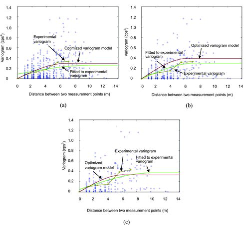
Figure 3 shows the variogram cloud, experimental variogram, variogram model optimally fitted to the experimental variogram (denoted as the fitted variogram model hereafter), and optimized variogram model for the cases involving (a) 30, (b) 25, and (c) 20 initial measurement points. As can be observed, the optimized variogram model is different from the fitted variogram model. This indicates that cross validation has provided more suitable model parameter values than the fitted variogram model. Table 2 lists the values of the three calculated parameters in the optimized variogram model. It is found that the nugget-effect established by the optimized variogram model is negligibly small in all cases. On the other hand, the nugget-effect is realized from the fitted variogram model except for the case involving 25 initial measurement points (Figure 3). It is noted that the range and sill values are similar but not equal among the three cases. This indicates that the variogram model parameters depend somewhat on the measurement points selected.

Table 2. Calculated values for the three parameters in the optimized variogram model for the area surrounding the Pu2 facility.

Case	Range (m)	Sill (cps^2)	Nugget-effect (cps^2)
30-1,2	6.62	0.290	8.60E-07
25-1,2	6.40	0.394	9.56E-07
20-1,2	6.13	0.332	1.76E-05

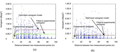
Figure 3. Variogram clouds, experimental variograms, optimally fitted variogram models for the experimental variograms, and optimized variogram models for the number of initial measurement points (NIMP) specified as (a) 30, (b) 25, and (c) 20.

5.1.3.2. Estimated mean, standard error, and distribution of counting rate

Table 3 lists the results for the estimated means, standard errors, and the ratios ${\sigma }_{n_0}/{\bar{z}}_{n_0}^{*}$ for the various NIMP considered, as calculated by MK-I, MK-II, and CSM. Each method yields nearly the same mean regardless of the NIMP employed. In contrast, the standard error has a tendency to increase with a decreasing NIMP. Regarding the estimated mean, CSM provides higher values than MK-I and MK-II. This is because the measurement points are not selected uniformly from the area but are biased in the region with higher counting rates. Therefore, the mean estimated by CSM is calculated using predominantly higher counting rate data. On the other hand, MK-I and MK-II account better for the lower counting rate data by utilizing spatial correlation effects. MK-I, in particular, considers the points over the entire area and estimates the mean by averaging all values in the area, as has been described in Section 3 and Appendix A.2. Therefore, even if the measurement points are biased, the results suggest that MK-I may provide a reasonable result for the estimated mean. It is noted that MK-II presents a larger standard error and ${\sigma }_{n_0}/{\bar{z}}_{n_0}^{*}$ than MK-I and CSM.

Table 3. Estimated means, standard errors, and ratios of standard error to mean for the area surrounding the Pu2 facility.

	Estimated mean	Estimated standard
Case	${\bar{z}}_{n_0}^{*}$ (cps)	error ${\sigma }_{n_0}$ (cps)	${\sigma }_{n_0}/{\bar{z}}_{n_0}^{*}$
30-1	0.408	0.0694	0.17
30-2	0.294	0.230	0.78
30-3	0.714	0.0814	0.11
25-1	0.415	0.0934	0.23
25-2	0.319	0.273	0.86
25-3	0.694	0.0888	0.13
20-1	0.402	0.0938	0.23
20-2	0.327	0.246	0.75
20-3	0.709	0.106	0.15

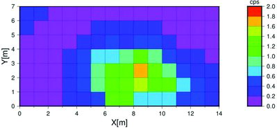
Figure 4 shows the estimated distribution of the counting rate of ¹³⁷Cs by ordinary kriging for an NIMP of 30. The figure indicates that the distribution in the survey unit is not uniform where a region exhibiting higher counting rates is observed around the center of the survey unit. The distribution ranges from ca. 0.1 to ca. 1.6 cps, which are one-fourth and quadruple of the mean (ca. 0.4 cps), respectively.

Figure 4. Estimated distribution of the counting rate of ¹³⁷Cs in cps obtained by ordinary kriging for 30 initial measurement points.

5.1.3.3. Comparison function and minimum number of measurement points required

Figure 5 shows the comparison functions (i.e., the left-hand side of Equation (16)) calculated by MK-I, MK-II, and CSM for an NIMP of (a) 30, (b) 25, and (c) 20. The figure indicates that MK-I provides the lowest value of the comparison function of the three methods, which results in the smallest value of n_min. The differences in the comparison functions between MK-I and CSM are mainly caused by the differences in estimated means because the standard errors are nearly equivalent, as has been shown in Table 3. Figures 6 and 7 show values of n_min as a function of the reference value for an NIMP of (a) 30, (b) 25, and (c) 20 (Figure 6) as calculated by (a) MK-I, (b) MK-II, and (c) CSM (Figure 7). It is observed that MK-II yields the largest value of n_min, whereas MK-I provides the smallest n_min value of the three methods, which suggests that MK-I leads to the most efficient measurement. The value of n_min depends strongly on the reference value, and n_min increases rapidly as the reference value decreases. This is understood from Figure 5 by considering that n_min is given by the point of intersection between the curve of the comparison function and the line y = d(¹³⁷Cs), and that the comparison function decreases gradually with increasing n. It is also observable that n_min is weakly dependent on the NIMP for MK-1 and CSM, but is more strongly dependent on it in the case of MK-II. This is because, in MK-II, σ(¹³⁷Cs)², which is equal to the sill parameter (see Table 2), and $\bar{\gamma }\left({}^{137}\mathrm{Cs}\right)$ (the values of $\bar{\gamma }\left({}^{137}\mathrm{Cs}\right)$ are 0.245, 0.333, and 0.286, for Case 30-2, Case 25-2, and Case 20-2, respectively) are somewhat different for Case 25-2 relative to Case 30-2 and Case 20-2, and because σ(¹³⁷Cs)² and $\bar{\gamma }\left({}^{137}\mathrm{Cs}\right)$ affect n_min, as is appreciated by consideration of Equation (40).

Figure 5. Comparisons of the calculated comparison functions with respect to the number of measurement points among MK-I, MK-II, and CSM for the number of initial measurement points (NIMP) specified as (a) 30, (b) 25, and (c) 20.

Figure 6. Comparison of the calculated minimum number of measurement points required as a function of the reference value among MK-I, MK-II, and CSM for the number of initial measurement points (NIMP) specified as (a) 30, (b) 25, and (c) 20.

Figure 7. Comparison of the calculated minimum number of measurement points required as a function of the reference value among the numbers of initial measurement points n₀ specified as 30, 25, and 20 by (a) MK-I, (b) MK-II, and (c) CSM.

5.2. Survey unit ID code: G51045E on the Trojan site

5.2.1. Objective area and data

Another sample case applied in this study is adopted from the site release experience data from the Trojan site [9] in the US. The Trojan nuclear power plant was a pressurized water reactor with the power of 1155 MWe. Construction of the plant began in 1970, commercial operation began in 1976, and the plant ceased operation permanently in 1993. The decommissioning of the plant began in 1996, and the site release terminated in 2005.

In the study, we use the measured radioactivity data taken from the soil of the survey unit ID code: G51045E denoted as the “Southeast Industrial Yard Area #3”. Figure 8 schematically describes the survey unit comprising 39 sections of section area 9 × 9 m². The radionuclides in question are ¹³⁷Cs and ⁶⁰Co. The concentration data of ¹³⁷Cs and ⁶⁰Co measured and evaluated at each section are listed in Table 4. It is observed that the measurement points are selected homogeneously, that the concentrations of ¹³⁷Cs and ⁶⁰Co are distributed rather uniformly, and are considerably lower than the corresponding DCGLs, which are 0.407 and 0.141 Bq/g for ¹³⁷Cs and ⁶⁰Co on the Trojan site, respectively.

Table 4. Radioactivity concentrations of ¹³⁷Cs and ⁶⁰Co at the survey unit on the Trojan site (data from [9], units were converted from pCi/g to Bq/g).

Section	^137Cs	^60Co	Section	^137Cs	^60Co
1	2.55E-03	2.74E-03	21	2.81E-03	2.07E-03
2	2.29E-03	2.59E-03	22	2.33E-03	2.18E-03
3	2.22E-03	2.29E-03	23	1.04E-03	2.48E-03
4	2.33E-03	2.22E-03	24	2.96E-03	3.03E-03
5	2.33E-03	2.04E-03	25	2.52E-03	2.22E-03
6	2.52E-03	2.92E-03	26	9.62E-04	2.29E-03
7	1.85E-03	2.59E-03	27	2.78E-03	3.48E-03
8	2.59E-03	2.55E-03	28	1.55E-03	2.26E-03
9	2.29E-03	2.00E-03	29	1.52E-03	2.55E-03
10	2.55E-03	1.89E-03	30	1.96E-03	2.55E-03
11	3.18E-03	3.11E-03	31	3.15E-03	2.70E-03
12	2.29E-03	2.29E-03	32	2.37E-03	2.37E-03
13	2.44E-03	2.33E-03	33	1.11E-03	2.37E-03
14	2.59E-03	2.55E-03	34	2.74E-03	2.48E-03
15	1.22E-03	2.55E-03	35	2.07E-03	2.48E-03
16	8.88E-04	2.00E-03	36	2.29E-03	2.48E-03
17	2.74E-03	2.52E-03	37	2.66E-03	2.89E-03
18	3.03E-03	2.52E-03	38	2.81E-03	3.00E-03
19	3.44E-03	2.26E-03	39	2.18E-03	2.15E-03
20	1.48E-03	3.15E-03

Figure 8. Objective area of the survey unit on the Trojan site (edited from [9]).

5.2.2. Calculation conditions

We applied the MK-I, MK-II, and CSM methods. The kriging calculations require that we define a mesh where the survey unit population is composed of the collection of all meshes, and the number of all meshes N in the survey unit is given by the survey unit area divided by the mesh area. We assume a mesh size of 30 × 30 cm², which provides 900 meshes for each section yielding a total of 35,100 meshes for the overall survey unit. The measurement point for each section is assumed to be located at the center of the section.

The calculation conditions for determining an optimized variogram model and the probabilities of Type I and Type II errors were the same as was applied to our study of the area surrounding the Pu2 facility. Because the ¹³⁷Cs and ⁶⁰Co concentrations of the Trojan site are too low to evaluate n_min, we used intentionally higher concentration values obtained by multiplying the original values by a scaling factor L, which was treated as a variable parameter.

Owing to the property of the kriging equation, for sample data multiplied by the factor L, the weighting factor based on the original data remains unchanged, whereas the Lagrange parameter based on the original data is multiplied by a factor L². As such, the estimated mean and the standard error values based on the original data are multiplied by L. Then equations calculating the minimum number for higher concentrations multiplied by L are given by $$\begin{array}{c}\sum _k\left(1-\frac{n}{N}\right)\left(\frac{1}{n}{\gamma }_{1w}\left(k\right)+\gamma \left(k\right)\right)/d{\left(k\right)}^2+C\left(f\right)\hfill \\ =& {\left(\frac{1/L-f_{n_0}^{*}}{k_{\alpha }+k_{\beta }}\right)}^2\hfill \end{array}$$and $$\begin{array}{c}\sum _k\left\{\sigma {\left(k\right)}^2-(1-1/n)\bar{\gamma }\left(k\right)\right\}/d{\left(k\right)}^2+C\left(f\right)\hfill \\ =& {\left(\frac{1/L-f_{n_0}^{*}}{k_{\alpha }+k_{\beta }}\right)}^2,\hfill \end{array}$$for MK-I and MK-II, respectively, with the use of results for L = 1. An equation for CSM is given by Equation (A.34) in Appendix B. We therefore conducted calculations for determining an optimized variogram model and for solving the kriging equations using the original data-set (i.e., for L = 1).

5.2.3. Results and discussion

5.2.3.1. The variogram model

Figure 9(a) and 9(b) shows variogram clouds, experimental variograms, fitted variogram models, and optimized variogram models for ¹³⁷Cs and ⁶⁰Co, respectively for L = 1. It is observed that the optimized variogram model for ¹³⁷Cs is different from the fitted variogram model. Values of three parameters, the nugget-effect, range, and sill, in the optimized variogram model are larger than those in the fitted variogram model. Especially the value of sill in the optimized variogram model is about twice as that in the fitted variogram model. This indicates that it is necessary to employ the cross validation and the optimized method for determining the appropriate variogram model. On the other hand, the optimized model for⁶⁰Co is equivalent to the fitted variogram model. This indicates that the initial values for the model parameters given by the fitted variogram model to optimize the variogram model happen to be the most suitable values. Experimental variograms for both radionuclides indicate that the variogram value becomes nearly equivalent when the points are slightly distanced from the origin, which suggests that there is little spatial correlation. Table 5 lists the values of the three calculated parameters in the optimized variogram models. It is observed that the nugget-effect is realized for the optimized variogram model for both radionuclides. This indicates that the values of the radionuclide concentration change abruptly at a very small scale.

Table 5. Calculated values for the three parameters in the optimized variogram model for the survey unit on the Trojan site with L = 1.

	Range	Sill	Nugget-effect
Radionuclide	(m)	[(Bq/g)^2]	[(Bq/g)^2]
^137Cs	13.5	8.74E-07	2.40E-07
^60Co	7.47	1.27E-07	8.43E-08

Figure 9. Variogram clouds, experimental variograms, optimally fitted variogram models for the experimental variograms, and optimized variogram models for (a) ¹³⁷Cs and (b) ⁶⁰Co with L = 1.

5.2.3.2. Estimated mean, standard error, and radioactivity distribution

Table 6(a) lists the results of the estimated means, standard errors, and the ratios ${\sigma }_{n_0}\left(k\right)/{\bar{z}}_{n_0}^{*}\left(k\right)$ for radioactivity concentrations of ¹³⁷Cs and ⁶⁰Co calculated by MK-I, MK-II, and CSM for L = 1, and Table 6(b) lists those of $f_{n_0}^{*}$, ${\sigma }_{n_0}\left(f_{n_0}^{*}\right)$, and ${\sigma }_{n_0}\left(f_{n_0}^{*}\right)/f_{n_0}^{*}$. Each method yields equivalent means within three significant figures. This is because the measurement points are distributed homogeneously and the distributions of radioactivity concentrations are nearly uniform. On the other hand, the standard errors presented by MK-II are larger than those by MK-I and CSM, which exhibits the same tendency as was observed in calculations of the area surrounding the Pu2 facility. It is observed that MK-I and CSM provide nearly equivalent results for both means and standard errors because of the minimal spatial correlation between the different points. Furthermore, it was observed that the calculated correlation effect C_f between ¹³⁷Cs and ⁶⁰Co, which could affect the value of n_min, was negligibly small at 1.63 × 10^{− 11}.

Table 6. Estimated means, standard errors, and ratios of standard error to mean for (a) concentrations of ¹³⁷Cs and ⁶⁰Co, and for (b) $f_{n_0}^{*}$ for the survey unit on the Trojan site with L = 1.

(a) Concentrations of ^137Cs and ^60Co
Radionuclide	Method	Estimated mean ${\bar{z}}_{n_0}^{*}$(Bq/g)	Estimated standard error ${\sigma }_{n_0}\left(k\right)$ (Bq/g)	${\sigma }_{n_0}\left(k\right)/{\bar{z}}_{n_0}^{*}$
^137Cs	MK-I	2.27E-03	9.83E-05	0.043
	MK-II	2.27E-03	1.73E-04	0.076
	CSM	2.27E-03	1.03E-04	0.045
^60Co	MK-I	2.49E-03	5.25E-05	0.021
	MK-II	2.49E-03	5.70E-05	0.023
	CSM	2.49E-03	5.63E-05	0.023
(b) $f_{n_0}^{*}$
Method	Estimated value $f_{n_0}^{*}$ (–)	Estimated standard error ${\sigma }_{n_0}\left(f_{n_0}^{*}\right)$ (–)	${\sigma }_{n_0}\left(f_{n_0}^{*}\right)/f_{n_0}^{*}$
MK-I	2.32E-02	4.44E-04	0.019
MK-II	2.32E-02	5.86E-04	0.025
CSM	2.32E-02	4.72E-04	0.020

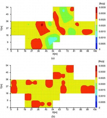
Figure 10(a) and 10(b) shows the distributions of the estimated radioactivity concentrations of ¹³⁷Cs and ⁶⁰Co, respectively, by ordinary kriging with L = 1. It is observed that the radioactivity concentrations of ¹³⁷Cs and ⁶⁰Co vary within a narrow range (from ca. 0.001 to ca. 0.003 (Bq/g) for ¹³⁷Cs and from ca. 0.002 to ca. 0.003 (Bq/g) for ⁶⁰Co). In other words, the distributions of both radionuclides in the survey unit are nearly uniform.

Figure 10. Estimated distributions of the radioactivity concentrations of (a) ¹³⁷Cs and (b) ⁶⁰Co by ordinary kriging with L = 1.

5.2.3.3. Comparison function and the minimum number of measurement points required

Figure 11 shows the comparison functions calculated by MK-I, MK-II, and CSM with L = 40. Differences among the results of the three methods in this case are observed to be less than the differences observed in the case of the area surrounding the Pu2 facility because of the minimal spatial correlation of the Trojan site. The MK-II result exhibits a somewhat higher value because of the larger standard error, which was also observed to be the case for the area surrounding the Pu2 facility. Figure 12 shows the value of n_min as a function of L calculated by MK-I, MK-II, and CSM. It is observed that the dependence of n_min on L significantly increases with increasing L, and the value of n_min calculated by MK-II becomes somewhat larger than that calculated by MK-I or CSM.

Figure 11. Comparison of the calculated comparison function with respect to the number of measurement points among MK-I, MK-II, and CSM with L = 40.

Figure 12. Comparison of the calculated minimum number of measurement points required as a function of L among MK-I, MK-II, and CSM.

5.3. Summary of results

The results calculated by MK-I, MK-II, and CSM for two sample cases are summarized as follows.

1. The optimized variogram models determined by the cross validation and optimized method were significantly different from the fitted variogram models in some cases. It is desirable to employ the optimized model in kriging calculations.

2. When the measurement points were not selected uniformly but selected from the region with higher counting rates data (the case of the area surrounding the Pu2 facility), the estimated mean by CSM was a higher value. However, the estimated mean by MK-I was reasonable because a spatial correlation between two different points could be considered. On the other hand, MK-II provided larger standard error of the estimated mean than MK-I and CSM. This results in decreasing the reliability of the estimated mean.

3. MK-I and CSM results showed minimum dependency of n_min on n₀, but MK-II results showed significant dependency. This means that the results by MK-I and CSM are more reliable than those by MK-II.

4. When there was little spatial correlation (the case of the survey unit on the Trojan site), MK-I and CSM provided similar results of the mean, standard error, and n_min. When there was spatial correlation and further when the measurement points were distributed inhomogeneously (the case of the area surrounding the Pu2 facility), MK-I provided smaller n_min than MK-II and CSM. This indicates that MK-I is a more efficient measurement method than MK-II and CSM.

6. Procedure for applying kriging to ensure compliance with release criterion

We here propose a procedure to determine if a survey unit complies with the site release criterion with consideration for Type I and Type II errors. In the proposed procedure, we assume that the radioactivity concentrations of radionuclides at some measurement points have been measured and evaluated. We omit a detailed procedure for estimating the mean radioactivity concentrations and standard errors of radionuclides in the survey unit that are obtained by solving the kriging equations under the variogram models determined, and focus on a procedure to apply the results. Through the application of kriging to the sample cases discussed in Section 5, it is suggested that MK-I is more appropriate than MK-II for use in ensuring compliance with the release criterion. Therefore, MK-I is employed in the following procedure. The procedure consists of three steps.

• Step 1: Estimate the mean radioactivity concentration ${\bar{z}}_{n_0}^{*}\left(k\right)$ and the standard error ${\sigma }_{n_0}\left(k\right)$ of each radionuclide by MK-I using a data-set of radioactivity concentrations obtained for n₀ measurement points in a survey unit.

• Step 2: Calculate $f_{n_0}^{*}$, ${\sigma }_{n_0}\left(f_{n_0}^{*}\right)$, and the comparison function with the controlled probabilities of Type I and Type II errors, α and β, respectively.

• Step 3: Compare the calculated value with the right-hand side value of Equation (15) or (16). If the calculated value is less than or equal to the right-hand side value, the survey unit is judged to be released. If the calculated value is larger than the right-hand side value, two options exist. One option (Option 1) is to add measurement points, and the other option (Option 2) is to conduct decontamination work on the survey unit. In Option 1, first calculate n_min for the case without consideration for measurement error. Second, set a somewhat larger number of measurement points n₁ than n_min, and add the measurement points to reach n₁. Third, return to Step 1 to obtain the revised mean radioactivity concentration ${\bar{z}}_{n_1}^{*}\left(k\right)$ and standard error ${\sigma }_{n_1}\left(k\right)$ using the measured data at both initial and added measurement points. In Option 2, after measuring and evaluating radioactivity concentrations for the decontaminated survey unit, return to Step 1 with the data-set for the survey unit reflecting lower radioactivity concentrations than those prior to decontamination.

7. Concluding remarks

In an effort to consider the spatial correlation of radioactivity concentrations between two points not considered in CSMs, we have discussed and proposed the application of two methods of kriging – MK-I and MK-II – considering the spatial correlation, to evaluate the mean radioactivity concentration for ensuring compliance with the site release criterion.

Because the estimated mean radioactivity concentration includes uncertainty that depends on the number of measurement points in a survey unit, site release should be determined with consideration for the decision error associated with this uncertainty to ensure public safety. We developed a method for calculating the uncertainty as a function of the number of measurement points. Furthermore, we derived equations to determine the minimum number of measurement points corresponding to the controlled error probability by revealing the relationship between ordinary kriging and MK-I, and using the properties of ordinary kriging (exact interpolator) and the variogram (where the value at the origin is zero).

We applied three methods, MK-I, MK-II, and CSM, to two sample cases. MK-I appropriately estimated the mean concentration even if the measurement points were distributed inhomogeneously over the survey unit (the case of the area surrounding the Pu2 facility), however MK-II and CSM estimated lower and higher values, respectively. Both of MK-I and CSM provided results of n_min that demonstrated a minimal dependence on the NIMP, which were desirable to apply the methods. The estimated standard error and n_min by MK-I were smaller than those calculated by MK-II, which suggests that MK-I leads to an efficient measurement. MK-I also provided a fewer number of measurement points than CSM when spatial correlation existed and further when the measurement points were distributed inhomogeneously (the case of the area surrounding the Pu2 facility). We therefore conclude that MK-I is a promising method that can be applied to ensure compliance with the site release criterion.

Appendix A. Kriging

A.1. Ordinary kriging

Ordinary kriging is employed for estimating the value of a physical quantity at a point of interest that has not been specifically subjected to measurement.

A.1.1. The variogram and kriging equation

In kriging, a variable corresponding to sample data such as radioactivity concentration obtained by measurement is treated as a random variable. Denoting a radioactivity concentration at a measurement point x_α(α = 1, …, n) in a survey unit as Z(x_α), the concentration at the point x_i is approximated by (A.1) $$Z^{*}\left({\mathbf{x}}_i\right)=\sum _{\alpha =1}^n{w}_{\alpha }^{i}Z\left({\mathbf{x}}_{\alpha }\right),$$(A.1) with the constraint condition (A.2) $$\sum _{\alpha =1}^n{w}_{\alpha }^i=1,$$(A.2) where indexes α and i represent numbers assigned to the measurement point and an arbitrary point, respectively, and wⁱ_α is a normalized weighting factor. The estimation variance is given by (A.3) $${\sigma }_E^2=\mathrm{var}[Z^{*}\left({\mathbf{x}}_i\right)-Z\left({\mathbf{x}}_i\right)],$$(A.3) where $\mathrm{var}\left[Z\right(\mathbf{x}\left)\right]$ denotes the variance of Z(x). The variation in space of Z(x) is described by taking the differences between values at pairs of points x and x + h: Z(x + h) − Z(x) [3]. Under the hypothesis of intrinsic stationarity of order 2, which consists of the two assumptions given by (A.4) $$E\left[Z\right(\mathbf{x}+\mathbf{h})-Z(\mathbf{x}\left)\right]=0$$(A.4) and (A.5) $$\mathrm{var}\left[Z\right(\mathbf{x}+\mathbf{h})-Z(\mathbf{x}\left)\right]=2\gamma \left(\mathbf{h}\right),$$(A.5) the theoretical variogram γ(h) is defined by (A.6) $$\gamma \left(\mathbf{h}\right)=E\left[{\{Z(\mathbf{x}+\mathbf{h})-Z\left(\mathbf{x}\right)\}}^2\right]/2,$$(A.6) where E[Z(x)] denotes the expectation value of Z(x). Using the least-squares method to minimize σ²_E under the condition of Equation (A.2), the equation for determining wⁱ_α at x_i (denoted as the kriging equation hereafter) is obtained as (A.7) $$\sum _{\beta =1}^n{w}_{\beta }^i\gamma ({\mathbf{x}}_{\alpha }-{\mathbf{x}}_{\beta })+{\mu }^i=\gamma ({\mathbf{x}}_{\alpha }-{\mathbf{x}}_i),$$(A.7) (A.8) $$\sum _{\alpha =1}^n{w}_{\alpha }^i=1,$$(A.8) where μⁱ is the Lagrange parameter. Using the solution of the kriging equation, the estimation variance is given by (A.9) $${\sigma }_E^2={\mu }^i-\gamma ({\mathbf{x}}_i-{\mathbf{x}}_i)+\sum _{\alpha =1}^n{w}_{\alpha }^i\gamma ({\mathbf{x}}_{\alpha }-{\mathbf{x}}_i).$$(A.9)

The theoretical variogram is not known, and an experimental variogram is introduced using sample data z(x_α)(α = 1, …, n) as (A.10) $$\widehat{\gamma }\left({\mathbf{h}}_k\right)=\frac{1}{2n\left({\mathbf{h}}_k\right)}\sum _{\alpha ,\beta =1}^n{\left\{z\left({\mathbf{x}}_{\alpha }\right)-z\left({\mathbf{x}}_{\beta }\right)\right\}}^2,$$(A.10) where h_k denotes a class that groups vectors whose lengths are within a specified interval of length and whose orientations are within a specified interval of angle, n(h_k) is the number of paired data belonging to the class h_k, and the sum is composed of the paired data. In the calculation of the experimental variogram, distance and orientation are both divided into several classes. An isotropic variogram is a function of only the distance, and is frequently used in practical calculations. Based on the experimental variogram, the theoretical variogram is approximated by a variogram model, which is expressed as a function of the distance of h = |h|. The variogram model depends on a model function and three parameters (a, b, c), and several variogram models have been proposed such as a spherical model, an exponential model, and a Gaussian model. The spherical model, for example, is given by $$\begin{array}{c}{\gamma }_M\left(h\right)=\hfill \\ \left\{\begin{array}{c}0\hfill \\ c+b\left\{3/2\times (h/a)-1/2\times {(h/a)}^3\right\}\\ c+b\end{array}\begin{array}{c}\mathrm{for}h=0\hfill \\ \mathrm{for}0<h\le a\hfill \\ \mathrm{for}h>a,\hfill \end{array}\right.\hfill \end{array}$$where a, b + c, and c are termed the range, the sill, and the nugget-effect, respectively.

A.1.2. Cross validation and determination of the variogram model

A variogram model is a key factor affecting the calculated results by kriging such as estimated values at points other than measurement points, standard errors of the estimated values, and estimated mean of the objective area. However, some arbitrariness exists in determining the model, i.e., its model function and parameters. Therefore, the question of how to choose the most appropriate model is significant. To determine parameters (a, b, c), an objective variable to be optimized should be assigned. Two candidates of objective variables are considered, one is the experimental variogram, and the other is the actual sample data. Regarding the former candidate, Pardo-Iguzquiza [12] discussed and developed a computer program using the simplex method of function minimization of Nelder and Mead [10]. However it is not possible to verify that the model obtained is the most appropriate because estimated values by kriging are not compared with the sample data. Regarding the latter candidate, cross validation is known to be an effective method. In this study, we employ cross validation and the simplex method to determine the variogram model.

Cross validation is summarized as follows. When a variogram model function is given, an estimated value of Z(x_i) at the point x_i, denoted by z*(x_i), is represented as a function of the three parameters (a, b, c): (A.11) $$z^{*}\left({\mathbf{x}}_i\right)=z^{*}(a,b,c;{\mathbf{x}}_i).$$(A.11)

Choosing the point x_i as a measurement point x_α and, in turn, solving the kriging equation at the point x_α using all other measurement points, we obtain an estimated value z*(a, b, c; x_α). We can then compare z*(a, b, c; x_α) with the corresponding actual data z(x_α). The values of the three parameters are determined as the magnitude of the mean squared cross-validation errors given by (A.12) $$Y=\frac{1}{n}\sum _{\alpha =1}^n{\left\{z\left({\mathbf{x}}_{\alpha }\right)-z^{*}(a,b,c;{\mathbf{x}}_{\alpha })\right\}}^2$$(A.12) is minimized.

A.2. Mean Kriging I

The mean of Z(x) over an area R of a survey unit is given by [7] (A.13) $$\bar{Z}=\frac{1}{R}{\int }_{R}d\mathbf{x}Z\left(\mathbf{x}\right),$$(A.13) where x varies within R. MK-I approximates the quantity $\bar{Z}$ by (A.14) $${\bar{Z}}_n^{*}=\sum _{\alpha =1}^n{\bar{w}}_{\alpha }Z\left(x_{\alpha }\right).$$(A.14)

Requiring that the expectation values of $\bar{Z}$ and ${\bar{Z}}^{*}$ are equal leads to the relation (A.15) $$\sum _{\alpha =1}^n{\bar{w}}_{\alpha }=1.$$(A.15)

In MK-I, the estimation variance is defined by the variance of the difference between the approximated mean and the true mean: (A.16) $$\begin{array}{c}\hfill {\sigma }_n^2={\sigma }_n{({\bar{Z}}_n^{*}-\bar{Z})}^2=E\left[{\left(\sum _{\alpha =1}^n{\bar{w}}_{\alpha }Z({\mathbf{x}}_{\alpha })-\frac{1}{R}{\int }_{R}d\mathbf{x}Z\left(\mathbf{x}\right)\right)}^2\right].\end{array}$$(A.16)

Minimizing the estimation variance under the condition of Equation (A.15), the kriging equation is given by (A.17) $$\sum _{\beta =1}^n{\bar{w}}_{\beta }\gamma ({\mathbf{x}}_{\alpha }-{\mathbf{x}}_{\beta })+\bar{\mu }=\frac{1}{R}{\int }_{R}d\mathbf{x}\gamma ({\mathbf{x}}_{\alpha }-\mathbf{x}),$$(A.17) (A.18) $$\sum _{\alpha =1}^n{\bar{w}}_{\alpha }=1.$$(A.18)

Here $\bar{\mu }$ represents the Lagrange parameter, and the estimation variance is given by (A.19) $$\begin{array}{ccc}\hfill {\sigma }_n^2& =& \bar{\mu }+\sum _{\alpha =1}^n{\bar{w}}_{\alpha }\frac{1}{R}{\int }_{R}d\mathbf{x}\gamma ({\mathbf{x}}_{\alpha }-\mathbf{x})\hfill \\ -\frac{1}{R^2}{\int }_{R}d\mathbf{x}d{\mathbf{x}}^{\text{'}}\gamma (\mathbf{x}-{\mathbf{x}}^{\text{'}}).\hfill \end{array}$$(A.19)

In a numerical calculation, the area R is divided into small area units denoted as meshes, and Equations (A.17) and (A.19) are rewritten as (A.20) $$\sum _{\beta =1}^n{\bar{w}}_{\beta }\gamma ({\mathbf{x}}_{\alpha }-{\mathbf{x}}_{\beta })+\bar{\mu }=\frac{1}{N}\sum _{i=1}^N\gamma ({\mathbf{x}}_{\alpha }-{\mathbf{x}}_i),$$(A.20) (A.21) $$\begin{array}{c}\hfill {\sigma }_n^2=\bar{\mu }+\sum _{\alpha =1}^n{\bar{w}}_{\alpha }\frac{1}{N}\sum _{i=1}^N\gamma ({\mathbf{x}}_{\alpha }-{\mathbf{x}}_i)-\frac{1}{N^2}\sum _{i,j=1}^N\gamma ({\mathbf{x}}_i-{\mathbf{x}}_j),\end{array}$$(A.21) where N is the total number of meshes in the survey unit.

A.3. Mean Kriging II

Mean kriging II approximates the mean of Z(x) over an area R of a survey unit by [3] (A.22) $${\bar{Z}}_n^{*}=\sum _{\alpha =1}^n{\bar{w}}_{\alpha }Z\left({\mathbf{x}}_{\alpha }\right).$$(A.22)

Requiring that expectation values of $\bar{Z}$ and ${\bar{Z}}^{*}$ are equal leads to the relation (A.23) $$\sum _{\alpha =1}^n{\bar{w}}_{\alpha }=1.$$(A.23)

In MK-II, the estimation variance is defined by (A.24) $$\sigma {\left({\bar{Z}}_n^{*}\right)}^2=\mathrm{E}\left[{\left(\sum _{\alpha =1}^n{\bar{w}}_{\alpha }Z({\mathbf{x}}_{\alpha })-m\right)}^2\right],$$(A.24) where m is the true mean. Minimizing the estimation variance under the condition of Equation (A.23), we obtain the kriging equation given by (A.25) $$\sum _{\beta =1}^n{\bar{w}}_{\beta }\gamma ({\mathbf{x}}_{\alpha }-{\mathbf{x}}_{\beta })+\bar{\mu }=0,$$(A.25) (A.26) $$\sum _{\alpha =1}^n{\bar{w}}_{\alpha }=1.$$(A.26)

Here $\bar{\mu }$ is the Lagrange parameter, and the estimation variance is given by (A.27) $${\sigma }_n^2={\sigma }_n{\left({\bar{Z}}_n^{*}\right)}^2={\sigma }^2-\sum _{\alpha ,\beta =1}^n{\bar{w}}_{\alpha }{\bar{w}}_{\beta }\gamma ({\mathbf{x}}_{\alpha }-{\mathbf{x}}_{\beta }),$$(A.27) where σ² is the variance of Z(x).

Appendix B. Statistical quantities in the conventional statistical method

We summarize the statistical quantities in the conventional statistical method that have been employed for calculations in Section 5, where measurement error is not considered. The presentation here uses the same notation as that used in the main text.

The estimated mean of the radioactivity concentration of a radionuclide and its standard error are given by (A.28) $${\bar{z}}_n^{*}=\sum _{\alpha =1}^{n}z\left({\mathbf{x}}_{\alpha }\right)/n,$$(A.28) (A.29) $${\sigma }_n=s_n/\sqrt{n},$$(A.29) with (A.30) $$s_n^2=\sum _{\alpha =1}^n{\left(z\left({\mathbf{x}}_{\alpha }\right)-{\bar{z}}_n^{*}\right)}^2/(n-1).$$(A.30)

The estimated value of F and its standard error are given by (A.31) $$f_n^{*}=\sum _k{\bar{z}}_n^{*}\left(k\right)/d\left(k\right),$$(A.31) (A.32) $${\sigma }_n\left(f_n^{*}\right)=\sqrt{{\sum }_k{\sigma }_n{\left(k\right)}^2/d{\left(k\right)}^2}.$$(A.32)

The minimum numbers of measurement points required for L = 1 and for higher concentration multiplied by L are given by (A.33) $$n_{min}=\frac{{(k_{\alpha }+k_{\beta })}^2}{{(1-f_{n_0}^{*})}^2}\sum _k{s}_{n_0}{\left(k\right)}^2/d{\left(k\right)}^2$$(A.33) and (A.34) $$n_{min}=\frac{{(k_{\alpha }+k_{\beta })}^2}{{(1/L-f_{n_0}^{*})}^2}\sum _k{s}_{n_0}{\left(k\right)}^2/d{\left(k\right)}^2,$$(A.34) respectively.

References

- Multi-agency radiation survey and site investigation manual (MARSSIM). Washington, DC: United States Department of Energy, Environmental Protection Agency, Nuclear Regulatory Commission and Department of Defense; 2000. (NUREG-1575, Rev.1, EPA 402-R-97-016, Rev.1, DOE/EH-0624, Rev.1).
- Decommissioning Safety Subcommittee, Nuclear Safety-Security Committee, Advisory Committee on Energy and Natural Resources. [Basic concept of decommissioning termination confirmation (interim report) – on main issues and direction of future discussion]. Tokyo, Japan: Ministry of Economy, Trade and Industry (METI); 2011. Japanese.
- Wackernagel H. Multivariate geostatistics: an introduction with applications. Berlin, Germany: Springer; 2003. ISBN 3-540-44142-5.
- Ishigami T, Shimada T. [Study on calculation method of the number of measurement points and procedure of decision-making for site release verification]. Tokai, Japan: Japan Atomic Energy Agency; 2014. (JAEA-Research 2013-048). Japanese.
- Berger JD. Manual for conducting radiological surveys in support of license termination. Oak Ridge, TN: Oak Ridge Associated Universities; 1992. (NUREG/CR-5849).
- Sukegawa T, Shimada T, Katsurai K, Tanaka T, Nakayama S. [Study on technical issues of site release of nuclear power plants – criteria for site release, procedures and verification requirements based on experiences in the U.S. – (contract research)]. Tokai, Japan: Japan Atomic Energy Agency; 2009. (JAEA-Review 2009-075). Japanese.
- Wang JF, Li LF, Christakos G. Sampling and kriging spatial means: efficiency and conditions. Sensors. 2009;9:5224–5240.
- Terunuma A, Naito A, Nemoto K, Usami J, Tomii H, Shiraishi K, Ito S. [Decommissioning five facilities in nuclear science research institute]. Tokai, Japan: Japan Atomic Energy Agency; 2010. (JAEA-Review 2010-038). Japanese.
- Trojan nuclear plant final survey report for support facilities and site grounds. Rainier, OR: Portland General Electric; 2004. (Docket 50-344).
- Nelder JA, Mead R. A simplex method for function minimization. Comput J. 1965;7:308–313.
- Dubrule O. Cross validation of kriging in a unique neighborhood. Math Geol. 1983;15:687–699.
- Pardo-Iguzquiza E. VARFIT: a fortran-77 program for fitting variogram models by weighted least squares. Comput Geosci. 1999;25:251–261.