Cross section adjustment method based on random sampling technique

Abstract

A cross section adjustment method based on the random sampling technique is proposed. In the proposed method, correlations among cross sections and core parameters are used instead of sensitivity coefficients of cross sections, which are necessary in the conventional method. The correlations are statistically estimated by the random sampling technique. The proposed method is theoretically consistent with the conventional method and provides comparable adjusted cross sections when sufficient number of random sampling is taken into account. The proposed method would be suitable for practical light water reactor (LWR) core analysis since estimation of sensitivity coefficients, which requires considerable computational cost in typical LWR problems, is not necessary. Through a benchmark problem in simple pin-cell geometry, adjusted cross sections by the present and the conventional cross section adjustment method are compared. The adjusted cross sections by the present method well reproduce the conventional ones, thus the feasibility of the present method is confirmed.

Keywords:

• cross section adjustment
• random sampling
• uncertainty
• covariance
• correlation

1. Introduction

Accurate prediction of core characteristics using core analysis is essential for safe and efficient operation of nuclear reactors. For higher prediction accuracy, reduction of uncertainties in core analysis is important. Uncertainties in core analysis consist of various factors, e.g., modeling of physical phenomena, approximations in numerical calculations, fabrication tolerance, and cross section data. They still have large impact on the results of core analysis though improvements of calculation methods and computer performances that has been going on. Among the above sources, uncertainties of cross sections could be a major contributor. Thus, estimation and reduction of uncertainties caused by uncertainties of cross sections is a major issue.

The cross section adjustment method is one of the techniques for improvement of prediction accuracy and reduction of uncertainties caused by cross sections [1,2]. The cross section adjustment method improves prediction accuracy of design core parameters by adjusting cross sections so that predicted neutronics characteristics well reproduce the measurement results in experiment. The cross section adjustment method has been widely applied to fast reactors. But its application to light water reactors (LWRs) is still limited because the typical calculation flow for LWR core analysis is rather complicated than that for fast reactors [3–5]. LWR core analysis includes complicated calculation flow with non-linear effect, e.g., lattice-core two-step calculation, thermal–hydraulics feedback calculation, and fine-step burn-up calculation. The complexity of the flow of LWR core analysis introduces difficulties for calculations of sensitivity coefficients, which is necessary to propagate cross section uncertainties and to perform cross section adjustment. Since numbers of input variables (i.e., number of energy groups multiplied by types of cross sections) and output variables (i.e., core characteristics and design parameters) are considerably large, both the forward and the adjoint-based approaches encounter difficulty in numerical calculations. Furthermore, the adjoint-based approach, which is commonly used for calculations of sensitivity coefficients, is not fully established for LWR analysis, including burn-up and thermal–hydraulics effects. Therefore, a new cross section adjustment method without estimation of sensitivity coefficients is highly desirable for practical applications of cross section adjustment to LWRs.

In this study, a cross section adjustment method based on the random sampling (RS) technique is proposed. The present method performs cross section adjustment without calculation of sensitivity coefficients but using correlations among cross sections and core parameters. The correlations among cross sections and core parameters are estimated by the RS technique using only forward calculations. In other words, the (generalized) adjoint calculation capability, which is not usually implemented in a typical core analysis system, is not necessary, thus the present method would facilitate application of cross section adjustment to LWRs. The present method offers three advantages. First, no (generalized) adjoint calculation is necessary. Second, accuracy of adjusted cross section can be appropriately chosen by the number of random samples thus the present method would be a practical approach for realistic problems. Finally, estimation of the sensitivity matrix, which requires large computational cost for typical LWR problems, is not necessary.

In Section 2, the theoretical background of the present method is described. In Section 3, numerical results of the present method compared with the conventional method using the sensitivity coefficients are shown. Finally, concluding remarks are summarized in Section 4.

2. Theory

2.1. Conventional cross section adjustment method

In this section, the conventional cross section adjustment method is described since it is a fundamental theory behind the present method [6]. A symbol P(X) is a prior probability for an event X and P(Y/X) is a posterior probability that an event Y is caused after the event X occurred. From the Bayes theorem, a relationship between a prior probability and a posterior probability is represented as: (1)

Using Equation (1), a posterior probability P(T/R_e) that the cross section set T takes the true value when the integral experimental data R_e is given, is written as: (2) where P(T) and P(R_e) are the prior probabilities that T and R_e take the true value, respectively, and P(R_e/T) is the posterior probability that R_e takes the true value under the condition that T is given.

In cross section adjustment method, it is assumed that a cross section set obeys a normal distribution and P(T) satisfies the following equation: (3) where T₀ is evaluated (nominal) value of cross sections; M is the covariance matrix of cross section set; and the superscript T means transposition. Equation (3) represents that the true value of cross section set has normal distribution around T₀ in a range of M.

Experimental data is also assumed to obey a normal distribution around the true value, thus P(R_e) satisfies the following equation: (4) where R_e0 is the true value of integral experimental data and V_e is the covariance matrix caused by experimental error. Moreover, it is assumed that P(R_e/T) is distributed around R_c(T), which is the predicted value of integral experiment, with a variance of V_e + V_m. It is noted that V_m is the covariance caused by the calculation method and no correlation is assumed between calculation and experimental errors. With these assumptions, the following equation holds: (5)

Substituting Equations (3)–(5) into Equation (2), the following equation is obtained: (6) where J(T) is defined as: (7)

Since the cross section set T does not appear in the denominator of Equation (6), the function J(T) should be minimized to maximize P(T/R_e). Hence, the adjusted cross section set should satisfy the following condition: (8)

Using the first-order approximation of the Taylor expansion, the calculation value R_c(T) is represented as: (9) where G is the sensitivity coefficient matrix for cross sections and consists of derivative coefficients of neutronics parameters around T₀. The function J(T) can be differentiated by substituting Equation (9) into Equation (7). By applying Equation (8) for T, the adjusted cross section set T_CA is finally derived as: (10)

In addition, M_CA, which is the covariance matrix of adjusted cross section T_CA, is obtained by calculating the variance of (T_CA − T₀) as: (11)

2.2. Random sampling technique for multivariate normal distribution

In this section, the typical theory of the RS technique for multivariate normal distribution is described, since it is one of the essential tools in the present method [7]. If a vector x consists of stochastic variables and it obeys the multivariate normal distribution with a mean vector μ and a covariance matrix Σ, x can be sampled by the following equation: (12) where z is a vector whose elements are independent random numbers of standard normal distribution N(0,1), and A is a square matrix that satisfies the following equation: (13)

Matrix A cannot be uniquely defined due to insufficient constraints but there are some numerical techniques for matrix decomposition shown in Equa-tion (13). In the present study, the singular value decomposition (SVD) method is used [8]. The covariance matrix Σ is decomposed as Equation (14) using the SVD since Σ is a real symmetric matrix: (14) where U is a unitary matrix whose columns are eigenvectors of Σ² and W is a diagonal matrix with singular values that corresponds to square roots of eigenvalues of Σ²: (15)

Since W is a nonnegative matrix, W is decomposed as follows: (16) where W^1/2 is (17)

By substituting Equation (16) into Equation (14), Σ is rewritten as: (18) where the mathematical properties of transpose matrix A^TB^T = (BA)^T and of diagonal matrix W^1/2 = (W^1/2)^T are utilized. Comparing Equation (18) with Equa-tion (13), the square matrix A in Equation (12) is obtained as (19)

Note that the matrix A written as Equation (19) is one of the matrixes that satisfy Equation (13) when the SVD is used. Finally, random sampling of stochastic variables x obeying the multivariate normal distribution with the mean vector μ and the covariance matrix Σ is carried out using the SVD as follows: (20)

In the following sections, x, μ and Σ correspond to a sampled cross section set T_i, an evaluated (i.e., nominal) value of cross section set T₀, and a covariance matrix of cross section set M, respectively.

2.3. Cross section adjustment method based on random sampling technique

As described in the Introduction, the most difficult part of cross section adjustment for LWRs is the estimation of the sensitivity coefficient matrix G for cross sections. Thus, in order to avoid this difficulty, we try to eliminate the sensitivity coefficient matrix G from Equation (10), which is the fundamental equation of the cross section adjustment method. The RS technique is used as an essential tool during the following theoretical derivation.

First, perturbed cross section sets T_1, T₂,…,T_N are obtained by random sampling with mean vector T₀ and covariance matrix M. N indicates the number of samples. The matrix ΔT, whose columns consist of variations of each sampled cross section set from T₀, is written as: (21)

Since T_1, T₂, … ,T_N are sampled using M, the covariance matrix estimated by statistical processing of T_1, T₂, … ,T_N should correspond to M. Therefore, if N is appropriately large, the following equation is satisfied: (22) where the right-hand side of Equation (22) represents statistical processing to estimate the covariance matrix. Note that unbiased variance is considered in Equation (22).

Secondary, predicted neutronics characteristics of integral experiment R_c(T₁), R_c(T₂), … ,R_c(T_N) are obtained by performing ordinary (i.e. forward) calculation with T₁, T₂, … ,T_N, respectively. The matrix ΔR, whose columns consist of variations of each predicted value from R_c(T₀), is written as: (23)

Then, introducing the sensitivity coefficient matrix G, the following relation between ΔT and ΔR is satisfied by applying the linear approximation: (24)

Based on the above equations, Equation (10) can be transformed. MG^T in Equation (10) is written as follows using Equation (22): (25) where the mathematical property of transpose matrix A^TB^T = (BA)^T is utilized. By substituting Equation (24) into Equation (25), MG^T is represented as (26)

Using Equation (22) and the property of transpose matrix, GMG^T in Equation (10) is also transformed as follows: (27)

Consequently, GMG^T is rewritten as follows by substituting Equation (24) into Equation (27): (28)

Finally, by substituting Equations (26) and (28) into Equation (10), the adjusted cross section set of the present method T’_CA is given by: (29)

Similarly, by substituting Equations (26) and (28) into Equation (11), M’_CA, which is the covariance matrix of T’_CA, is given by: (30)

2.4. Discussion

Differences between the conventional and the proposed methods are represented only by Equations (26) and (28). The elements of ΔT and ΔR, defined in Equations (21) and (23), respectively, can be expressed as follows: (31) (32) where the subscript n is the number of elements in cross section set and m is the number of elements in core parameter set. In other words, n is generally equal to the number of cross section types multiplied by the number of energy groups, m corresponds to the number of target core parameters. Equations (26) and (28) can be expressed as follows: (33) (34) where T_1, T₂, … ,T_n are elements in cross section set T and R₁, R₂, … ,R_m are elements in core parameter set R. Symbols of var(X) and cov(X,Y) represent variance of X and covariance between X and Y, respectively. It is noted that the variances and covariances in Equations (33) and (34) are caused by the uncertainties of cross sections. Equations (33) and (34) suggest that the present cross section adjustment method utilizes covariances among cross sections and core parameters, and covariances (or variances) among core parameters. In the conventional cross section adjustment method, they are estimated by propagating uncertainties of cross sections using the sensitivity coefficient matrix G. In the present method, on the other hand, they are statistically estimated withfinite samples of ΔT and ΔR using the RS technique. This is the major difference between the conventional and the proposed methods. Both methods include linear approximation between cross sections and core parameters, which is shown in Equations (9) and (24), respectively. Additionally, the proposed method includes statistical approximation in the evaluation of covariance among cross sections shown in Equation (22), covariance among cross sections and core parameters shown in Equation (33), and covariance among core parameters shown in Equation (34). The approximations shown in Equations (22), (33), and (34) indicate these statistical approximations.

The present and the conventional methods have different characteristics from the viewpoint of computational cost. For the conventional method, G should be evaluated by sensitivity calculations. In this case, considerable computational cost is necessary unless some technique is used. For estimation of sensitivity coefficients, there are mainly two approaches. One is the forward-based approach that uses forward calculations with perturbed cross sections. The other is the adjoint-based approach that uses adjoint calculations based on the generalized perturbation theory. The number of forward or adjoint calculations is identical to the number of cross sections types or the number of core characteristics, respectively. In practical LWR problems, the number of cross section types or core characteristics is considerably large. On the contrary, for the proposed method, only ΔR should be evaluated instead of G. Note that ΔT is generated during the application of the RS technique. The most important point is that, an arbitrary number of forward calculations can be used to evaluate ΔR. Therefore, the proposed method could be a feasible approach especially for practical problems considering many cross sections and core characteristics. However, accuracy of the adjusted cross section will depend on the number of samples since the present method is essentially a stochastic approach. Validity and accuracy of the present method will be confirmed through a benchmark problem in the next section.

3. Numerical verification

In order to verify the present cross section adjustment method based on the RS technique, a verification calculation is carried out. The present and conventional methods are applied to a simple pin-cell calculation with virtual integral experimental data. In the present paper, we focus on the verification of the fundamental feasibility of the present method.

3.1. Verification condition

In this verification calculation, the CASMO-4 code is used and multi-group microscopic cross sections provided in L-library, which is a 70-group microscopic cross section library for CASMO-4, are used for adjustment [9]. Types of reaction cross section for adjustment include capture, fission, scattering, number of neutrons per fission (ν) of U-235 and capture and scattering of U-238. Thus, the total number of cross sections for adjustment is 420 (= 70 × 6; “70” and “6” is the number of energy groups and types of reaction, respectively).

The number of core parameter is one and only a k-infinity of pin-cell at beginning of life is considered. A typical PWR pin-cell, which consists of fuel (UO₂), gap, cladding, and moderator (light water), is used. Pin-cell configuration and calculation conditions are shown in Tables 1 and 2. A part of them is taken from unit cell specification of TMI-1 in the UAM benchmark problem [10].

Table 1. Configuration of fuel pin-cell.

Parameter	Value
Fuel pellet material	UO2
Fuel density [g/cm^3]	10.283
Fuel enrichment [wt%]	4.85
Fuel pellet diameter [mm]	9.391
Cladding material	Zircaloy-2
Cladding outside diameter [mm]	10.928
Cladding thickness [mm]	0.673
Unit cell pitch [mm]	14.427

Table 2. Conditions of pin-cell calculation.

Parameter	Value
Fuel temperature [K]	900
Moderator temperature [K]	600
Cladding temperature [K]	636
Boron concentration [ppm]	0

Actual measurement data of integral experiment are not used in this verification. Instead, k-infinity obtained by a pin-cell calculation using a randomly sampled cross section set is considered as the virtual “experimental” value. Using the virtual experimental value, cross section adjustment is carried out by the present and the conventional method. Thus, when the adjusted cross sections by the present method reproduces well those by the conventional method, the present cross section adjustment can be considered as a feasible method at least for a small-scale problem.

The number of maximum samples in the RS technique is 500, that is to say, 500 sets of perturbed L-library for CASMO-4 are generated by the RS technique and 500 pin-cell calculations are carried out by CASMO-4 with perturbed L-libraries. In order to investigate the impact of the number of samples on the adjusted cross section, the present cross section adjustment is carried out with various numbers of samples from 5 to 500 (5, 10, 20, 30, 40, 50, 100, 200, 500) by altering the number of samples considered in the matrixes ΔT and ΔR described in Section 2.3. In other words, only five pin-cell calculation results are used in the coarsest cross section adjustment but 500 results are used in the finest adjustment case.

For the comparison of the present and conventional cross section adjustment methods, the conventional method using the sensitivity coefficients is carried out with the identical calculation conditions. Sensitivity coefficient matrix G is obtained by forward sensitivity calculations where each cross section is directly perturbed. Each sensitivity coefficient is calculated by the centered difference approximation, that is to say, ∂R_c(T₀)/∂T_i, which is the sensitivity coefficient of the core parameter R_c(T₀) to the focused cross section T_i, is evaluated as: (35) where x represents perturbation of T_i, and R_c(T_i,+x) and R_c(T_i,−x) are the calculated values with perturbed cross sections, respectively. In this verification, each cross section is perturbed by 5% to estimate the sensitivity coefficient by Equation (35).

Details of each vector or matrix used in this verification are described as follows:

• T₀ is the cross section in L-library and the number of elements is 420 (= 70 × 6).

• R_c(T) is obtained by a pin-cell calculation with T and the number of elements is 1.

• M is derived from the covariance data of JENDL-4.0u [11,12]. The covariance data for each nuclide and reaction are processed into the 70 group structure for L-library by the NJOY code and the results of the NJOY code is rearranged to M whose size is 420 × 420 matrix [13].

• ΔT is obtained by the RS technique using T₀ and M, and is 420 × N matrix (N is number of randomly sampled cross section sets).

• ΔR is obtained by pin-cell calculations with perturbed cross section sets that are generated by the RS technique, and is 1 × N matrix.

• G is obtained by pin-cell calculations with the perturbed (± 5%) cross section, and is 1×420 matrix. Note that G is not necessary for the present cross section adjustment but is used for the conventional cross section adjustment for comparison.

• R_e is the virtual “experimental” value of k-infinity. It is obtained by a pin-cell calculation with a cross section set, which is generated by the additional random sampling.

• V_e and V_m are assumed to be zero matrixes for simplicity in the present study. However, these covariance matrixes would have considerable impact in actual applications. Thus, further study considering V_e and V_m will be desirable using actual experimental (measurement) values as R_e.

Finally, differences of the adjusted cross sections by the present and the conventional methods are evaluated to verify feasibility of the proposed method. When the differences of the adjusted cross sections by the present and the conventional methods are small, the present adjustment method is considered as feasible. Moreover, calculation values of k-infinity with the adjusted cross sections are also evaluated to confirm the adequacy of the adjusted cross sections.

3.2. Results

In Table 3, k-infinity obtained by the adjusted cross section sets of the conventional and the present methods and their differences from the virtual experimental value are shown. The virtual experimental value of k-infinity is 1.28652, which is the target value. In Table 3, “Conventional” means the conventional cross section adjustment method using the sensitivity coefficients and “Number of samples” means the number of random samples used in the present method. The difference of k-infinity with the unadjusted cross section is the order of 10⁻³, but is reduced to the order of 10⁻⁵ with the adjusted cross section. The differences of k-infinity with the adjusted cross sections by the present method are comparable regardless of the number of samples. The present result shows the fundamental adequacy of the present method since cross sections are adjusted to reproduce the virtual experimental value. However, in order to confirm the validity of the present method, adjusted cross sections should be compared with those obtained by the conventional method.

Table 3. k-infinity and their differences from the virtual experimental value.

			After adjustment
			Present
	Virtual experimental value	Before adjustment	5	50	200	500	Convectional
k-infinity	1.28652	1.27703	1.28655	1.28651	1.28652	1.28653	1.28655
Difference	–	−9.5×10^−3	3×10^−5	−1×10^−5	0	1×10^−5	3×10^−5

Note: Difference is defined by (calculation value)–(virtual experimental value). Each of 5, 50, 200, and 500 means the number of random samples in the present method.

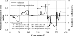
Next, the variations of cross sections by the conventional method are shown in Figure 1 with sensitivity coefficients. Here, the variation of cross section represents the difference between the adjusted and the unadjusted cross section. The scale for variations of cross sections is normalized by the standard deviations of each unadjusted cross section. For example, when the variation of a cross section (i.e., the difference between the adjusted and the unadjusted cross section) equals to the standard deviation of the cross section, it is shown as 1.0 in Figure 1. The horizontal axis shows each cross section in order of energy group (Cross section ID: 1∼70 = U-235 capture, 71∼140 = U-235 fission, 141∼210 = U-235 scattering, 211∼280 = U-235 ν, 281∼350 = U-238 capture, 351∼420 = U-238 scattering). Figure 1 indicates that the cross sections, whose sensitivity is relatively large (e.g. U-235 ν, U-238 capture), are adjusted. This is a characteristic of the cross section adjustment method that minimizes variation of cross sections.

Figure 1. Variations of cross sections by the conventional method (normalized by standard deviation of cross section) and sensitivity coefficients.

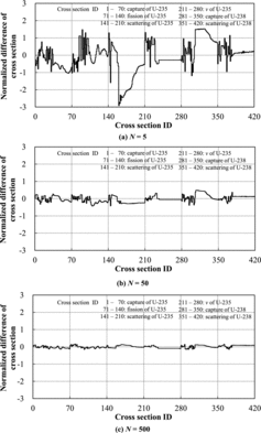
Then the differences of adjusted cross sections obtained by the present and the conventional methods are shown in Figure 2. The vertical axis of Figure 2 is also normalized by the standard deviation of each cross section. In the present verification, we focus on the differences of adjusted cross section between the present and the conventional methods since the “true” cross section cannot be reproduced even by the conventional method in the present benchmark condition. Figure 2 indicates that the differences of adjusted cross sections are large in a small sample case, i.e., when N = 5; N means the number of samples. On the other hand, the differences of adjusted cross sections are small in a large sample case, i.e., when N = 500. This result suggests that the adjusted cross sections obtained by the present method are comparable to those obtained by the conventional method when the sufficient number of samples is taken in the RS technique. The differences of the adjusted cross sections are within one standard deviation of cross section uncertainty when N = 50. Thus, appropriate adjustment of cross sections would be possible with only tens of random samples in this verification condition, which is clearly smaller than the number of cross section types, i.e., 420. In other words, we can expect further computational efficiency of the present method than that of the conventional method using forward-based sensitivity calculations. It should be reminded that sensitivity coefficients for k-infinity without burn-up and thermal–hydraulics feedback can be easily estimated through an adjoint calculation. However, in actual LWR problems, we should evaluate the sensitivity coefficients of core parameters including nonlinear burn-up and thermal–hydraulics feedback effect. Application of the adjoint theory would be difficult in this situation; thus, the finite–difference approximation with forward calculations would be necessary to estimate the sensitivity coefficients. The present method could be adequate for such a situation.

Figure 2. Differences of adjusted cross sections of the proposed method from those of the conventional method for 5, 50, and 500 samples. The vertical axis is normalized by the standard deviation of cross section.

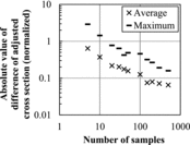
In the present method, accuracy of the adjusted cross section depends on the number of samples. Figure 3 shows the average and maximum differences of the adjusted cross sections between the present and the conventional methods for various numbers of samples. Note that an absolute value of the differences of the adjusted cross sections is considered and then the average and maximum of the absolute values are shown in Figure 3. Figure 3 clearly shows that the adjusted cross sections by the present method converge to those by the conventional method as the number of samples increases. This result means the equivalence of the present and the conventional methods. It is noted that the adjusted cross sections would not precisely converge to those obtained by the conventional method. Since the sensitivity coefficients used in the conventional method are approximately estimated by the direct perturbation with finite difference approximation thus the adjusted cross sections by the conventional method are not the rigorous ones.

Figure 3. The average and maximum differences of adjusted cross sections obtained by the present and the conventional methods for various numbers of samples. The vertical axis is normalized by the standard deviation of cross section.

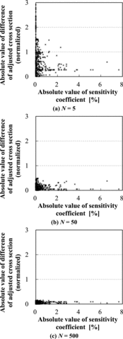
In the above results, k-infinity obtained by the adjusted cross section (N = 5) in Table 3 reproduces well the virtual experimental value, but the adjusted cross sections show considerable difference in Figure 2. These results suggest that the cross sections that have strong impact on a core parameter (k-infinity in this study) tend to be adequately adjusted even if the number of samples is relatively small. Figure 4 shows the relationship between the absolute value (magnitude) of the sensitivity coefficient and the difference of the adjusted cross section obtained by the conventional and the present methods. Apparently, the cross sections with large sensitivity coefficients are appropriately adjusted even if the number of samples is small. On the contrary, the cross sections with small sensitivity coefficients show larger discrepancy for small sample case. Anyway, difference of the adjusted cross section between the conventional and the present methods reduces for all range of sensitivity coefficients as the number of samples increases. The above results suggest that the present method tends to appropriately adjust cross sections with large sensitivity coefficients since correlation between a cross section with large sensitivity coefficient and a core parameter is easily estimated by statistical analysis through the random sampling technique.

Figure 4. Relationship between differences of adjusted cross sections by the present and the conventional methods and sensitivity coefficients. The vertical axis is normalized by the standard deviation of cross section.

4. Conclusion

The cross section adjustment method based on the random sampling technique is proposed. In the present method, two covariance matrixes are statistically estimated using the random sampling technique, i.e., the covariance among cross sections and core parameters, and the covariance among core parameters. These two covariance matrixes are used in the cross section adjustment instead of the sensitivity coefficients in the conventional cross section adjustment. The present method has three advantages. First, no (generalized) adjoint calculation is necessary, which is not usually implemented in common core analysis codes. Second, accuracy of adjusted cross section can be controlled by the number of random samples thus the present method would be a practical approach for realistic problems. Finally, estimation of the sensitivity matrix is not necessary, which requires large computational resources for typical LWR problems.

The proposed method is applied for pin-cell calculations with simple calculation conditions where the number of cross section types is 420 and the numbers of core parameters is 1. The virtual experimental value of k-infinity, which is calculated by a perturbed cross section set, is used as a target parameter. The conventional cross section adjustment is also carried out for comparison. The results indicate that the proposed cross section adjustment appropriately reproduces the adjusted cross sections obtained by the conventional method when the number of samples used in the random sampling technique is appropriate. Thus feasibility of the proposed method is confirmed.

In the present method, accuracy of the adjusted cross sections depends on the number of samples. In this study, which takes only 420 cross sections and 1 core parameter into consideration, cross sections are appropriately adjusted with tens of samples, which is practical. However, appropriate number of samples would be increased for a practical problem such as LWR core analysis, which should take more cross sections and core parameters into consideration, because the estimation accuracy of covariance matrixes among cross sections and core parameters, among core parameters could depend on the numbers of cross sections and core parameters to be considered. Moreover, the complicated process of LWR core analysis, e.g., energy group collapsing and homogenization of cross section, burn-up calculation, and thermal–hydraulic feedback, might have some impact on the results of adjustment. However, since the present method uses only forward calculations, there would be no particular difficulty in the application of the present method to LWR core analysis. Applicability of the present method to practical LWR problems will be confirmed as a future study.

Additional information

Funding

This work was supported in part by JSPS KAKENHI, Grant-in-Aid for Scientific Research [(C) (24561040)].

References

- Dragt JB, Dekker JWM, Guppelaar H, Janssen AJ. Methods of adjustment and error evaluation of neutron capture cross sections. Application to fission product nuclides. Nucl Sci Eng. 1977; 62:117.
- Takeda T, Yoshimura A, Kamei T. Prediction uncertainty evaluation methods of core performance parameters in large liquid-metal fast breeder reactors. Nucl Sci Eng. 1989;103:157.
- Abdel-khalik HS. Adaptive core simulation [dissertation]. Raleigh: North Carolina State University; 2004.
- Jessee MA, Turinsky P, Abdel-khalik HS. Many-group cross-section adjustment techniques for boiling water reactor adaptive simulation. Nucl Sci Eng. 2011 Sep; 169: 40–55.
- Kato S, Endo T, Yamamoto A, Yamauchi H, Kimura Y. Random sampling-based cross-section adjustment technique for LWR core analysis. Paper presented at: Proceedings ICAPP 2013; 2013 Apr 14–18; Jeju Island, Korea. [CD-ROM].
- Yokoyama K, Ishikawa M, Kugo T. Extended cross-section adjustment method to improve the prediction accuracy of core parameters. J Nucl Sci Technol. 2012;49:1165–1174.
- Muirhead RJ. Aspects of multivariate statistical theory. New York: John Wiley & Sons; 1982.
- Bai Z, Demmel J, Dongarra J, Ruhe A, van der Vorst H. Templates for the solution of algebraic eigenvalue problems: a practical guide. Philadelphia: SIAM; 2000.
- CASMO-4 A Fuel Assembly Burn-up Program. User's Manual. SSP-09/443 - U Rev 0: Studvik Scandpower, Inc: 2009.
- Ivanov K, Avramova M. Benchmark for Uncertainty Analysis in Modeling (UAM) for design, operation and safety analysis of LWRs. NEA/NSC/DOC(2007)23: Nuclear Energy Agency; 2007.
- Shibata K, Iwamoto O, Nakagawa T, Iwamoto N, Ichihara A, Kunieda S, Chiba S, Furukawa K, Otuka N, Ohsawa T, Murata T, Matsunobu H, Zukaran A, Kameda S, Katakura J. JENDL-4.0: A new library for nuclear science and engineering. J Nucl Sci Technol. 2011 Jan; 48:1–30.
- JENDL-4.0u. Available from: http://wwwndc.jaea.go.jp/jendl/j40/update/. Japan Atomic Energy Agency; 2013.
- Macfarlane RE, Muir DW. The NJOY Nuclear Data Processing System Version 91. LA-12740-M; October 1994.