Correction of count-loss effect in neutron correlation methods that employ single neutron counting system for subcriticality measurement

Abstract

It is well known that the count-loss effect produces serious problems for the neutron correlation methods that employ a single neutron counting system, e.g. the variance-to-mean and the auto-correlation methods, since it deteriorates the information extracted from the subcritical reactor system. New formulae of the variance-to-mean and auto-correlation methods were hence obtained on the basis of a rigorous theoretical approach for treating the count-loss process. It is expected that the present formulae work better than conventional ones for determination of the neutron decay constant.

Keywords:

• neutron correlation method
• variance-to-mean (or Feynman-α) method
• auto-correlation (or Rossi-α) method
• count-loss effect
• neutron decay constant
• subcriticality
• measurement
• nuclear criticality safety

1. Introduction

Measurement of subcriticality (i.e. negative reacti-vity) is one of the most important subjects in the field of reactor physics since it is closely related to the nuclear criticality safety. The neutron correlation methods that can measure the subcriticality through determination of the neutron decay constant [1–7] are useful tools and have been applied to many subcritical reactor systems [8–14]. Investigations on neutron correlation methods are still being pursued to meet a renewed necessity of subcriticality measurement (or monitoring) for accelerator-driven systems [15–27]. In future research works on criticality management of fuel debris generated in a severe accident of light water reactors [28], it is expected that the neutron correlation methods will play an important role.

In the neutron correlation methods, the temporal fluctuation in neutron population is of interest and is measured by using the neutron counting system that consists of a neutron detector and instrumentation circuits. Researchers have, however, revealed that the variance-to-mean (or the Feynman-α) method that employs a single neutron counting system often fails to determine the neutron decay constant owing to the count-loss effect [12,29,30]. Several authors tackled this problem and obtained different formulae of the variance-to-mean method with a correction of the count-loss effect [12,20,31,32].

The semi-empirical formula by Yamane and Ito [31] is one of thus obtained and has been frequently used in recent years [29,30,33–35]. However, the concrete expression of the factor D, which is included in their semi-empirical formula to empirically take the count-loss process into account, is obscure. Hence, no one has verified their semi-empirical formula yet. Likewise, the formula of the auto-correlation (or the Rossi-α) method based on the semi-empirical approach of Yamane and Ito has not been verified, since it also includes the unknown factor D. In the present paper, hence, on the basis of not empirical approaches but a rigorous theoretical one for treating the count-loss process [36], new and alternative formulae of the variance-to-mean and auto-correlation methods with a correction of the count-loss effect are obtained.

Brief reviews of the variance-to-mean and auto-correlation methods are provided in the following section. The one-time-point and two-time-point neutron observation probabilities that explicitly consider the count-loss process are then derived in Section 3. By using the neutron observation probabilities thus derived, the new formulae of the variance-to-mean and auto-correlation methods with a correction of the count-loss effect are obtained in the same section. Verification of neutron observation probabilities by a series of Monte Carlo calculations is described in Section 4. The present new formulae are also verified in the same section. Finally, the conclusion is summarized in Section 5.

2. Brief reviews of the variance-to-mean and auto-correlation methods

2.1. Variance-to-mean method

It is well known that there are two different types of models for the count-loss process that correspond to the idealized responses of a radiation counting system, i.e. the paralyzable and the non-paralyzable ones [37]. In the present paper, the paralyzable count-loss process is considered for simple discussion. We would like to mention here that the real counting system involves a count-loss process that is not one of either of these two models but an intermediate one between them. However, the difference between these two models is small when the frequency of neutron capture events in a neutron detector is low, so that this assumption leads to few problems for this region.

Let us suppose a zero-power subcritical reactor system that contains an extraneous stationary neutron source and J sets of neutron counting systems. One understands that considering the case of J = 1 is enough for the present paper since the neutron correlation methods that employ a single neutron counting system are discussed. However, the multiple neutron counting systems are considered throughout for the convenience of future works that will be dealing with two or more counting systems.

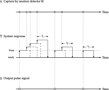
Each neutron counting system is supposed to be composed of a neutron detector and instrumentation circuits and to involve the paralyzable count-loss process with dead time τ_j (j = 1, 2, … , J). It is well known that such a neutron counting system cannot generate the output pulse signal for τ_j after every neutron capture event in the neutron detector, as illustrated in Figure 1 [37]. As a result, the number of neutrons “observed” disagrees with that of neutrons “captured” by a neutron detector when the frequency of capture events in the neutron detector is high. One hence often fails to acquire the accurate information on the temporal fluctuation in neutron population that is required by the neutron correlation methods.

Figure 1. Illustration of the paralyzable count-loss process.

In the variance-to-mean (or the Feynman-α) method, the number of neutrons observed by a single neutron counting system within a certain length of gate width is repeatedly registered to quantify the temporal fluctuation in neutron population by the correlation index Y_var, i.e. the variance-to-mean ratio of the number of neutrons observed minus unity: (1) where and are the first- and second-order moments of the number of neutrons observed by the jth neutron counting system within the gate width T. These two kinds of moment quantities can be calculated as (2) (3) where p_j(t₁)dt₁ is the one-time-point neutron observation probability that one neutron is observed within an infinitesimal time interval dt₁ around t₁, and p_{j, j}(t₁, t₂)dt₁dt₂ the two-time-point probability that a pair of neutrons are observed within respective infinitesimal time intervals dt₁ around t₁ and dt₂ around t₂ (t₁ < t₂).

In 1949, within the one-point reactor approximation model with one group of neutron energy and no delayed neutrons, de Hoffmann derived the one-time-point and two-time-point neutron observation probabilities without considering the count-loss process [38]: (4) (5) with the following notations: (6) (7) (8) (9) (10) (11) where S is the intensity of the extraneous stationary neutron source, α the neutron decay constant, ρ the reactivity, Λ the neutron generation time, λ_c the probability that one neutron is captured per unit time by materials excluding the neutron detectors in the subcritical reactor system, λ_f the probability that one neutron undergoes a fission reaction per unit time, λ_{d, j} the probability that one neutron is captured per unit time by the jth neutron detector, v the velocity of neutrons, and Σ_x the macroscopic cross-sections of corresponding interaction types x = c, f, d. The notations ⟨ν⟩ and ⟨ν(ν − 1)⟩ are the first two factorial moments of the number of neutrons generated per fission reaction and are defined as (12) (13) where (14) is the probability that n neutrons are generated per fission reaction.

By substituting Equations (4(4) ) and (5(5) ) into Equations (1(1) )–(3(3) ), one obtains Y_var without any correction of the count-loss effect as (15) where (16) This is the original formula of the variance-to-mean method that was used in the first experiment by Feynman et al. [8].

On the basis of the idea proposed by Srinivasan and Sahni [39,40], Yamane and Ito modified the one-time-point and two-time-point neutron observation probabilities as follows [31]: (17) (18) where the factor D_j ranges from zero to unity and takes unity when the dead time τ_j is zero to empirically take a reduction of the frequency of neutron observation due to the count-loss process into consideration. Owing to the count-loss process, no neutrons are observed during (t₁, t₁ + τ_j) under the condition that one neutron is observed at time t₁. Hence, p_{j, j}(t₁, t₂)dt₁dt₂ for 0 ≤ t₂ − t₁ < τ_j is set to be zero in Equation (18(18) ). By substituting Equations (17(17) ) and (18(18) ) into Equations (1(1) )–(3(3) ), the formula of the variance-to-mean method with a correction of the count-loss effect is hence obtained as follows: (19) with the following notations: (20) (21) where the superscript is the abbreviation for semi-empirical. This semi-empirical formula has been frequently used by many researchers in recent experiments [29,30,33–35].

2.2. Auto-correlation method

In the auto-correlation (or the Rossi-α) method, the number of neutrons observed within (t₁ − Δ₀ + Δ, t₁ + Δ) under the condition that one neutron is observed at time t₁ is registered to quantify the temporal fluctuation in neutron population by the auto-correlation function R_auto, where Δ is the time after the observation of a neutron at t₁, and Δ₀ the fundamental time interval corresponding to the coincidence gate of Orndoff’s instrumentation circuits [9]. The auto-correlation function with respect to the jth neutron counting system thus measured can be calculated as follows: (22) By substituting Equations (4(4) ) and (5(5) ) into Equation (22(22) ), one obtains R_auto (Δ₀ ≤ Δ) without any correction of the count-loss effect as (23) where (24) (25) This is the original formula of the auto-correlation method that was used in the first experiment by Orndoff [9]. On the other hand, on the basis of the semi-empirical approach of Yamane and Ito, by substituting Equations (17(17) ) and (18(18) ) into Equation (22(22) ), the formula of the auto-correlation method with a correction of the count-loss effect is obtained as follows: (26) (27) (28) One finds that this semi-empirical formula is practically equivalent to the original one when one determines the neutron decay constant by the least-square fitting technique.

3. New formulae with a correction of the count-loss effect

3.1. Degweker’s formulation

In 1989, Degweker paid attention to the fact that the jth neutron counting system that involves the paralyzable count-loss process with dead time τ_j can generate an output pulse signal at time t when the neutron detector captures no neutrons within the preceding time interval (t − τ_j, t), and developed a rigorous formulation approach for treating the count-loss process [36] on the basis of the backward master equation formalism [18,41–43]. 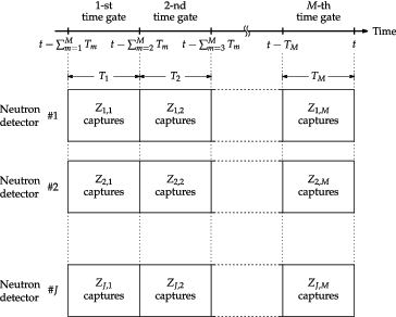In the present paper, to derive the one-time-point and two-time-point neutron observation probabilities by Degweker’s formulation, the following probability is introduced: (29) where (30) (31) (32) This is the source-induced probability that Z_{j, m} neutrons are captured by the jth neutron detector (j = 1, 2, … , J) within the mth time gate (m = 1, 2, … , M) under the condition that an extraneous stationary neutron source is introduced into the subcritical reactor system at time 0, and t the closing time of the Mth time gate. Here, as illustrated in Figure 2, the time gates that have respective durations T_m (m = 1, 2, … , M) are supposed to be mutually adjacent and non-overlapping.

Figure 2. Timing diagram of .

According to Degweker’s formulation, the one-time-point neutron observation probability is derived by introducing of two-interval version (M = 2). As illustrated in Figure 3, one derives the one-time-point neutron observation probability with respect to the jth neutron counting system, i.e. 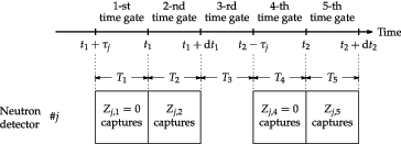p_j(t₁)dt₁, as the expectation of the number of neutron capture events in the jth neutron detector within an infinitesimal time interval dt₁ around t₁ under the condition that no neutrons are captured within the preceding time interval (t₁ − τ_j, t₁) that is observed in a steady state realized by the extraneous stationary neutron source after a long waiting time: (33) where (34) (35) On the other hand, as illustrated in Figure 4, one similarly derives the two-time-point neutron observation probability p_{j, j}(t₁, t₂)dt₁dt₂ by introducing of five-interval version (M = 5) as (36) (37) One easily understands that no neutrons can be observed during (t₁, t₁ + τ_j). Hence, p_{j, j}(t₁, t₂)dt₁dt₂ for 0 ≤ t₂ − t₁ < τ_j is set to be zero in Equation (36(36) ).

Figure 3. Timing diagram of the one-time-point neutron observation probability p_j(t₁)dt₁.

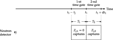
Figure 4. Timing diagram of the two-time-point neutron observation probability p_{j, j}(t₁, t₂)dt₁dt₂.

As seen in Equations (33(33) ) and (36(36) ), one understands that the one-time-point and two-time-point neutron observation probabilities can be derived when the analytical expression of is obtained. In Degweker’s formulation, however, one does not obtain but the following probability generating function for simple mathematical manipulation: (38) (39) where (40) Using of two-interval version, Equation (33(33) ) can be rewritten as follows: (41) (42) where T′ is given in Equation (35(35) ). On the other hand, Equation (36(36) ) can be rewritten by using of five-interval version as (43) (44) where T′ is given in Equation (37(37) ).

In the following subsections, to derive the one-time-point and two-time-point neutron observation probabilities that explicitly consider the count-loss process, the analytical expression of is obtained within the one-point reactor approximation model with one group of neutron energy and no delayed neutrons.

3.2. Source-induced probability generating function

Let us introduce the following probability: (45) This is the source-induced probability that Z_{j, m} neutrons are captured by the jth neutron detector (j = 1, 2, … , J) within the mth time gate (m = 1, 2, … , M) under the condition that the extraneous stationary neutron source is introduced into the subcritical reactor system at time t₀, and t the closing time of the Mth time gate (t₀ ≤ t). The terminal condition of is read as (46) The corresponding probability generating function and its terminal condition are as follows: (47) (48) Let us further introduce another probability, (49) (50) This is the single-particle-induced probability that Z_{j, m} neutrons are captured by the jth neutron detector (j = 1, 2, … , J) within the mth time gate (m = 1, 2, … , M) under the condition that an initial neutron is injected into the subcritical reactor system at time 0, and t the closing time of the Mth time gate.

Let us consider where introduction of the extraneous stationary neutron source is delayed by Δt0. Assuming that the time interval (t0, t0 + Δt0) is small enough to neglect any two-fold source events, one can establish the following probability balance equation [43]: (51) where (52) (53) Multiplying xZ1, 11, 1xZ1, 21, 2⋅⋅⋅xZJ, MJ, M and then performing a summation from zero to infinity with respect to Z1, 1, Z1, 2, … , ZJ, M, one obtains the following equation from Equation (51(51) ): (54) where (55) (56) By letting Δt0 → 0 after some rearrangement, the following differential equation is obtained: (57)

This equation can be solved with the terminal condition given in Equation (48(48) ), i.e. (58) where (59) (60) When setting t₀ = 0, the following equation: (61) is obtained. Therefore, by substituting Equation (61(61) ) into Equation (38(38) ), is obtained as (62)

In the following subsection, the analytical expression of g(x, T, t) that is included on the right-hand side of Equation (62(62) ) is obtained by considering the elementary processes of neutron interactions in a subcritical reactor system.

3.3. Single-particle-induced probability generating function

Let us consider P(Z, T, t − Δt) where injection of an initial neutron is delayed by Δt. Neglecting any two-fold neutron interactions within an infinitesimal time interval (0, Δt), the following probability balance equation can be established [18]: (63) The respective terms on the right-hand side correspond to mutually exclusive neutron interactions within (0, Δt). Here, R_n(Z, T, t) is the multi-particle-induced probability that Z_{j, m} neutrons are captured by the jth neutron detector (j = 1, 2, … , J) within the mth time gate (m = 1, 2, … , M) under the condition that n neutrons are simultaneously injected at time 0, and t the closing time of the Mth time gate. This probability can be easily constructed with P(Z, T, t). For example, R_n(Z, T, t) with respect to n = 0, 1, 2, 3 are written as follows: (64) (65) (66) (67) where (68) (69) On the other hand, by using Heaviside’s step function H(t), Δ_m(t) is defined as (70) where (71) This function is introduced to describe the status of time gate by taking zero when closed or unity when opened. Furthermore, is defined as follows: (72)

Multiplying xZ1, 11, 1xZ1, 21, 2⋅⋅⋅xZJ, MJ, M and then performing a summation from zero to infinity with respect to Z1, 1, Z1, 2, … , ZJ, M, one obtains the following equation from Equation (63(63) ): (73) Hence, the following backward master equation is obtained by making some rearrangement and then letting Δt → 0: (74) Rewriting Equation (74(74) ) by using g(x, T, t), the Pál–Bell equation [41,42] of J-detector and M-interval version is obtained as (75) where ⟨ν(ν − 1)(ν − 2)⋅⋅⋅(ν − r + 1) ⟩ is the rth-order factorial moment of the number of neutrons generated per fission reaction which is defined as (76)

To solve the Pál–Bell equation of J-detector and M-interval version, the two-forked approximation that neglects the components of order higher than third of the second term on the right-hand side of Equation (75(75) ) is introduced, i.e. (77) Regarding the two-forked approximation, Furuhashi and Izumi pointed out that the contributions from higher order components than third are negligible except in reactor systems with far large subcriticalities [44,45].

To solve Equation (77(77) ) efficiently, let us divide g(x, T, t) into M + 1 regions as (78) (79) (80) with the following boundary conditions: (81) Although Equation (79(79) ) is non-linear, it is of Ricatti type that can be solved analytically. One hence obtains the solution as follows: (82) (83) (84) (85) Therefore, one can now perform an integration on the right-hand side of Equation (62(62) ) as (86) (87) The analytical expression of is hence obtained as (88)

As seen in subsection 3.1, of two-interval and five-interval versions are required to derive the one-time-point and two-time-point neutron observation probabilities. The concrete expressions of Γ(x, T) of respective versions, i.e. Γ₂(x, T) and Γ₅(x, T), are hence provided as follows: (89) (90)

3.4. One-time-point neutron observation probability

In this subsection, the one-time-point neutron observation probability p_j(t₁)dt₁ is derived by substituting Equations (88(88) ) and (89(89) ) into Equation (41(41) ).

The T₂ → dt₁ limitation of of two-interval version is calculated as the Maclaurin expansion with elimination of higher order terms of dt₁ as (91) where (92) (93) Therefore, by substituting Equation (91(91) ) into Equation (41(41) ), p_j(t₁)dt₁ is derived as follows: (94) (95) (96)

To verify the one-time-point neutron observation probability derived, let us substitute τ_j = 0. As a result, it becomes identical to Equation (4(4) ).

3.5. Two-time-point neutron observation probability

In this subsection, the two-time-point neutron observation probability p_{j, j}(t₁, t₂)dt₁dt₂ is derived by substituting Equations (88(88) ) and (90(90) ) into Equation (43(43) ).

The T₂ → dt₁ and T₅ → dt₂ limitations of of five-interval version are calculated as the Maclaurin expansion with elimination of higher order terms of dt₁ and dt₂ as follows: (97)

where (98) (99)

(100) (101)

(102)

(103) Therefore, by substituting Equation (97(97) ) into Equation (43(43) ), p_{j, j}(t₁, t₂)dt₁dt₂ is derived as follows: (104) (105) (106)

To verify the two-time-point neutron observation probability derived, let us substitute τ_j = 0. As a result, it becomes identical to Equation (5(5) ).

3.6. New formulae of the variance-to-mean and auto-correlation methods

To obtain new formulae of the variance-to-mean and auto-correlation methods with a correction of the count-loss effect, let us suppose ατ_j ≪ 1 and then approximate , , and as (107) (108) (109) Typical values of α and τ_j in actual experiments for measuring the neutron decay constant are 10¹ ∼ 10⁵ s⁻¹ and less than 10 μs, respectively. It is hence expected that this approximation would be widely applicable.

Using Equations (107(107) )–(109(109) ) in Equations (94(94) ) and (104(104) ), one obtains the new formula of the variance-to-mean method with a correction of the count-loss effect from Equations (1(1) )–(3(3) ) as follows: (110) where (111) (112) (113) One finds here that the present formula of the 0th-order approximation is practically equivalent to the semi-empirical one obtained by Yamane and Ito when one determines α by the least-square fitting technique.

On the other hand, the new formula of the auto-correlation method with a correction of the count-loss effect is obtained from Equation (22(22) ) as follows: (114) where (115) (116) (117) One finds here that the present formulae of the 0th- and first-order approximations are practically equivalent to the original and semi-empirical ones for determination of α.

4. Discussions

4.1. Verification of neutron observation probabilities

To verify the one-time-point and two-time-point neutron observation probabilities derived in the previous section, a series of mono-energy analogue Monte Carlo calculations, where a typical thermal subcritical reactor system for neutron correlation methods with subcriticality of 3%Δk/k and neutron decay constant of 1566.3 s⁻¹ was supposed, was carried out. The parameters for these Monte Carlo calculations are listed in Table 1. In these Monte Carlo calculations, the time of every neutron capture event in respective neutron detectors was tallied to obtain time series data. By simulating the paralyzable count-loss process [37], the time-series data thus obtained were converted into those with respect to various dead times τ_j. We would like to mention here that the binomial-type distribution by Diven et al. [46] was supposed in determining the number of neutrons generated per fission reactionand the intensity of an extraneous stationary neutron source S was selected so as to result in R_j = 1.0 × 10³, 1.8 × 10³, … , 1.0 × 10⁵ s⁻¹.

Table 1. Parameters for Monte Carlo calculations.

Parameter	Value
λc (s^−1)	33196.2315
λf (s^−1)	21685.7490
λd (s^−1)	334.8504
λd, j (s^−1)	λd/2 (j = 1, 2)
J	2
p(n):	0.0329091534 (n = 0)
	0.1611584430 (n = 1)
	0.3156817007 (n = 2)
	0.3091831067 (n = 3)
	0.1514091461 (n = 4)
	0.0296584501 (n = 5)
S (s^−1)	, , , ,
	, , , ,
τj (μs)	2, 4, 6, 8, 10 (j = 1, 2)
Δ0 (s)	1.0 × 10^−5

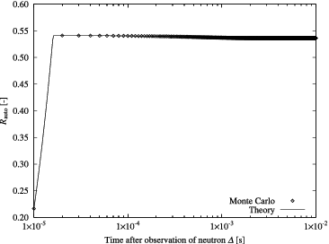
In Figures 5–7, examples of Y_var curves of the variance-to-mean method obtained by the Monte Carlo calculations are shown. To efficiently obtain the Y_var curves, the bunching technique was introduced [13]. On the other hand, examples of R_auto curves of the auto-correlation method are provided in Figures 8–10. Corresponding theoretical curves calculated on the basis of the one-time-point and two-time-point neutron observation probabilities and the parameters listed in Table 1 are also plotted in these figures. The integral in Equation (3(3) ) and that in Equation (22(22) ) could not be obtained analytically, so that they were evaluated numerically by the trapezoidal rule. In these figures, one confirms that the theoretical curves based on neutron observation probabilities agree well with those by the Monte Carlo calculations.

Figure 5. Example of Y_var curves calculated by Monte Carlo and theory (R_j = 1.0 × 10³ s⁻¹, τ_j = 2 μs).

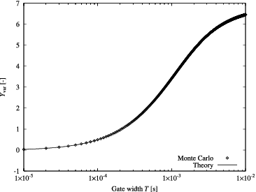
Figure 6. Example of Y_var curves calculated by Monte Carlo and theory (R_j = 1.0 × 10⁴ s⁻¹, τ_j = 4 μs).

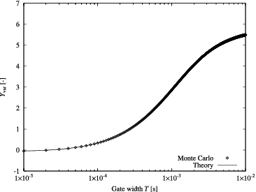
Figure 7. Example of Y_var curves calculated by Monte Carlo and theory (R_j = 1.0 × 10⁵ s⁻¹, τ_j = 6 μs).

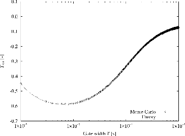
Figure 8. Example of R_auto curves calculated by Monte Carlo and theory (R_j = 1.0 × 10³ s⁻¹, τ_j = 2 μs).

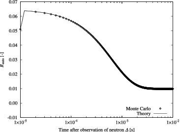
Figure 9. Example of R_auto curves calculated by Monte Carlo and theory (R_j = 1.0 × 10⁴ s⁻¹, τ_j = 4 μs).

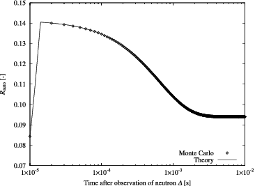
Figure 10. Example of R_auto curves calculated by Monte Carlo and theory (R_j = 1.0 × 10⁵ s⁻¹, τ_j = 6 μs).

4.2. Verification of the new formulae

To verify the formulae obtained in the previous section, the theoretical curves with respect to Y_var and R_auto that were calculated on the basis of the one-time-point and two-time-point neutron observation probabilities and the parameters listed in Table 1 were plotted again, and then α was determined by the least-square fitting technique using Equations (110(110) ) and (114(114) ) as well as the original formulae given in Equations (15(15) ) and (23(23) ) and the semi-empirical ones given in Equations (19(19) ) and (26(26) ). We would like to mention here that the fitting parameters of the present formula of the variance-to-mean method were for the 0th-order approximation, for the first-order approximation, and for the second-order approximation. Similarly, the fitting parameters of the present formula of the auto-correlation method were for the 0th- and first-order approximations, and for the second-order approximation. The deviations of the determined α from the reference are tabulated in Table 2 for the variance-to-mean method and in Table 3 for the auto-correlation method.

Table 2. Deviation of α determined by formulae of the variance-to-mean method from the reference.

		Deviation from the reference α (%)
Rj (s^−1)	Formula^*	τj = 2 μs	τj = 4 μs	τj = 6 μs	τj = 8 μs	τj = 10 μs
1.0 × 10^3	Orig	−1.373	−2.694	−3.965	−5.184	−6.365
	S-E/0th	+0.013	+0.038	+0.089	+0.160	+0.243
	First	+0.013	+0.051	+0.115	+0.198	+0.300
	Second	+0.000	+0.000	+0.000	+0.000	+0.000
1.8 × 10^3	Orig	−1.539	−3.026	−4.456	−5.848	−7.202
	S-E/0th	+0.013	+0.045	+0.102	+0.179	+0.275
	First	+0.013	+0.057	+0.128	+0.223	+0.338
	Second	+0.000	+0.000	+0.000	+0.000	+0.000
3.2 × 10^3	Orig	−1.832	−3.614	−5.357	−7.055	−8.728
	S-E/0th	+0.013	+0.057	+0.121	+0.217	+0.332
	First	+0.019	+0.070	+0.153	+0.268	+0.409
	Second	+0.000	+0.000	+0.000	+0.000	+0.000
5.6 × 10^3	Orig	−2.362	−4.693	−7.004	−9.309	−11.601
	S-E/0th	+0.019	+0.070	+0.160	+0.281	+0.434
	First	+0.019	+0.089	+0.198	+0.345	+0.536
	Second	+0.000	+0.000	+0.000	+0.000	+0.000
1.0 × 10^4	Orig	−3.320	−6.685	−10.119	−13.624	−17.213
	S-E/0th	+0.026	+0.102	+0.230	+0.409	+0.632
	First	+0.032	+0.128	+0.281	+0.504	+0.779
	Second	+0.000	+0.000	+0.000	+0.000	−0.006
1.8 × 10^4	Orig	−5.082	−10.483	−16.242	−22.390	−28.966
	S-E/0th	+0.038	+0.160	+0.364	+0.658	+1.047
	First	+0.045	+0.198	+0.447	+0.811	+1.290
	Second	+0.000	+0.000	+0.000	−0.006	−0.013
3.2 × 10^4	Orig	−8.415	−18.094	−29.190	−41.816	−56.033
	S-E/0th	+0.064	+0.268	+0.645	+1.219	+2.056
	First	+0.077	+0.332	+0.792	+1.494	+2.522
	Second	+0.000	+0.000	−0.006	−0.013	−0.032
5.6 × 10^4	Orig	−15.016	−34.617	−59.377	−89.999	N/A
	S-E/0th	+0.115	+0.511	+1.341	+2.918	+5.950
	First	+0.140	+0.626	+1.647	+3.575	+7.253
	Second	+0.000	+0.000	−0.013	−0.051	−0.185
1.0 × 10^5	Orig	−29.081	−74.411	N/A	N/A	N/A
	S-E/0th	+0.217	+1.181	+4.386	+19.658	+104.673
	First	+0.268	+1.449	+5.363	+23.310	+104.897
	Second	+0.000	−0.006	−0.083	−1.283	−3.422

Note: ^* “Orig” and “S-E” mean the original formula and the semi-empirical one, respectively.

Table 3. Deviation of α determined by formulae of the auto-correlation method from the reference.

		Deviation from the reference α (%)
Rj (s^−1)	Formula^*	τj = 2 μs	τj = 4 μs	τj = 6 μs	τj = 8 μs	τj = 10 μs
1.0 × 10^3		+0.019	+0.077	+0.166	+0.287	+0.434
	Second	+0.000	+0.000	+0.000	+0.000	+0.000
1.8 × 10^3		+0.019	+0.083	+0.185	+0.319	+0.492
	Second	+0.000	+0.000	+0.000	+0.000	+0.000
3.2 × 10^3		+0.026	+0.102	+0.223	+0.383	+0.587
	Second	+0.000	+0.000	+0.000	+0.000	−0.006
5.6 × 10^3		+0.032	+0.128	+0.287	+0.504	+0.773
	Second	+0.000	+0.000	+0.000	+0.000	−0.006
1.0 × 10^4		+0.045	+0.185	+0.409	+0.728	+1.130
	Second	+0.000	+0.000	+0.000	−0.006	−0.006
1.8 × 10^4		+0.070	+0.281	+0.645	+1.168	+1.858
	Second	+0.000	+0.000	+0.000	−0.006	−0.019
3.2 × 10^4		+0.115	+0.479	+1.143	+2.164	+3.633
	Second	+0.000	+0.000	−0.006	−0.026	−0.057
5.6 × 10^4		+0.204	+0.913	+2.388	+5.152	+10.362
	Second	+0.000	−0.006	−0.026	−0.096	−0.351
1.0 × 10^5		+0.383	+2.100	+7.693	+31.641	+106.040
	Second	+0.000	−0.019	−0.153	−1.864	+4.393

Note: ^* “Orig” and “S-E” mean the original formula and the semi-empirical one, respectively.

Regarding the original formula of the variance-to-mean method, one finds a clear dependency on the dead time τ_j and the source intensity S, i.e. as τ_j and S are become larger, this formula brings a larger underestimation and finally fails to determine α. On the other hand, it is seen that the present formula of the 0th-order approximation (that is practically equivalent to the semi-empirical one by Yamane and Ito) and that of the first-order approximation give better results, although the latter provides worse results than the former. One further finds that the present formula of the second-order approximation always provides the best results. A similar result is observed also in Table 3; the present formula of the second-order approximation works best.

5. Conclusion

On the basis of not empirical approaches but a rigorous theoretical one, one-time-point and two-time-point neutron observation probabilities that explicitly consider the count-loss process were derived and verified by a series of Monte Carlo calculations. By introducing an approximation that would be widely applicable to actual experiments for measuring the neutron decay constant into the neutron observation probabilities thus derived, new and alternative formulae of the variance-to-mean and auto-correlation methods were obtained. It is expected that the present formulae of the second-order approximation work better than conventional ones for determination of the neutron decay constant.

Acknowledgements

The authors would like to express their thanks to Dr Yasunobu Nagaya for his careful examination and valuable comments.

Notes

1. The probability that n neutrons are generated per fission reaction was defined by the following distribution: where n_max and ⟨ν⟩ are the maximum and the first-order moments of the number of neutrons generated. They were set to be 5 and 2.474, respectively.

References

- Thie JA. Reactor noise. New York (NY): Rowman & Littlefield; 1963.
- Pacilio N. Reactor-noise analysis in the time domain (TID-24512). Oak Ridge (TN): US Atomic Energy Commission/Division of Technical Information; 1969.
- Saito K. Rozatsuon-no-riron (I) [Theory of reactor noise (I)] (JAERI 1187). Tokyo: Japan Atomic Energy Research Institute; 1970.
- Uhrig RE. Random noise techniques in nuclear reactor systems. New York (NY): Ronald Press; 1970.
- Otsuka M. Genshiro-butsuri [Nuclear reactor physics]. Tokyo: Kyoritsu Shuppan; 1972.
- Williams MMR. Random processes in nuclear reactors. Oxford: Pergamon Press; 1974.
- Pázsit I, Pál L. Neutron fluctuations: a treatise on the physics of branching processes. Amsterdam: Elsevier; 2008.
- Feynman RP, de Hoffman F, Serber R. Dispersion of the neutron emission in U-235 fission. J Nucl Energy. 1956;3:64–69.
- Orndoff JD. Prompt neutron periods of metal critical assemblies. Nucl Sci Eng. 1957;2:450–460.
- Albrecht RW. The measurement of dynamic nuclear reactor parameters using the variance of the number of neutrons detected. Nucl Sci Eng. 1962;14:153–158.
- Gotoh Y. Measurement of neutron life in a D2O-system by neutron fluctuation. J Nucl Sci Technol. 1964;1:193–196.
- Edelmann M, Ehrhardt J, Väth W. Investigations of the two-detector covariance method for the measurement of coupled reactor kinetics parameters. Ann Nucl Energy. 1975;2:207–216.
- Misawa T, Shiroya S, Kanda K. Measurement of prompt neutron decay constant and large subcriticality by the Feynman-α method. Nucl Sci Eng. 1990;104:53–65.
- Por G, Szappanos G. Feynman-alpha measurement in a 100kW research reactor. Prog Nucl Energy. 1998;33:439–455.
- Pázsit I, Yamane Y. Theory of neutron fluctuations in source-driven subcritical systems. Nucl Instruments Methods Phys. Res. Section A. 1998;403:431–441.
- Pázsit I, Yamane Y. The variance-to-mean ratio in subcritical systems driven by a spallation source. Ann Nucl Energy. 1998;25:667–676.
- Yamane Y, Pázsit I. Heuristic derivation of Rossi-alpha formula with delayed neutrons and correlated source. Ann Nucl Energy. 1998;25:1373–1382.
- Pázsit I, Yamane Y. The backward theory of Feynman- and Rossi-alpha methods with multiple emission sources. Nucl Sci Eng. 1999;133:269–281.
- Behringer K, Wydler P. On the problem of monitoring the neutron parameters of the fast energy amplifier. Ann Nucl Energy. 1999;26:1131–1157.
- Degweker SB. Some variants of the Feynman alpha method in critical and accelerator driven subcritical systems. Ann Nucl Energy. 2000;27:1245–1257.
- Kitamura Y, Yamauchi H, Yamane Y. Derivation of variance-to-mean formula for periodic and pulsed neutron source. Ann Nucl Energy. 2003;30:897–909.
- Kitamura Y, Yamauchi H, Yamane Y, Misawa T, Ichihara C, Nakamura H. Experimental investigation of variance-to-mean formula for periodic and pulsed neutron source. Ann Nucl Energy. 2004;31:163–172.
- Pázsit I, Kitamura Y, Wright J, Misawa T. Calculation of the pulsed Feynman-alpha formulae and their experimental verification. Ann Nucl Energy. 2005;32:986–1007.
- Kitamura Y, Taguchi K, Misawa T, Pázsit I, Yamamoto A, Yamane Y, Ichihara C, Nakamura H, Oigawa H. Calculation of the stochastic pulsed Rossi-alpha formula and their experimental verification. Prog Nucl Energy. 2006;48:37–50.
- Kitamura Y, Pázsit I, Wright J, Yamamoto A, Yamane Y. Calculation of the pulsed Feynman- and Rossi-alpha formulae with delayed neutrons. Ann Nucl Energy. 2005;32:671–692.
- Kitamura Y, Misawa T, Yamamoto A, Yamane Y, Ichihara C, Nakamura H. Feynman-alpha experiment with stationary multiple emission sources. Ann Nucl Energy. 2006;48:569–577.
- Kitamura Y, Taguchi K, Yamamoto A, Yamane Y, Misawa T, Ichihara C, Nakamura H, Oigawa H. Application of variance-to-mean technique to subcriticality monitoring for accelerator-driven subcritical reactor. Int J Nucl Energy Sci Tech. 2006;2:266–284.
- Izawa K, Uchida Y, Ohkubo K, Totsuka M, Sono H, Tonoike K. Infinite multiplication factor of low-enriched UO2-concrete system. J Nucl Sci Technol. 2012;49:1043–1047.
- Hashimoto K, Ohya K, Yamane Y. Experimental investigations of dead time effect on Feynman-α method. Ann Nucl Energy. 1996;23:1099–1104.
- Kitamura Y, Matoba M, Misawa T, Unesaki H, Shiroya S. Reactor noise experiments by using acquisition system for time series data of pulse train. J Nucl Sci Technol. 1999;36:653–660.
- Yamane Y, Ito D. Feynman-α formula with dead time effect for a symmetric coupled-core system. Ann Nucl Energy. 1996;23:981–987.
- Hazama T. Practical correction of dead time effect in variance-to-mean ratio measurement. Ann Nucl Energy. 2003;30:615–631.
- Wallerbos EJM, Hoogenboom JE. The forgotten effect of the finite measurement time on various noise analysis techniques. Ann Nucl Energy. 1998;25:733–746.
- Wallerbos EJM, Hoogenboom JE. Experimental demonstration of the finite measurement time effect on the Feynman-α technique. Ann Nucl Energy. 1998;25:1247–1252.
- Kitamura T, Misawa T, Unesaki H, Shiroya S. General formulae for the Feynman-α method with the bunching technique. Ann Nucl Energy. 2000;27:1199–1216.
- Degweker SB. Effect of deadtime on the statistics of time correlated pulses – application to the passive neutron assay problem. Ann Nucl Energy. 1989;16:409–416.
- Knoll GF. Radiation detection and measurement. 2nd ed. New York (NY): Wiley; 1979; p. 95–99.
- de Hoffmann F. The science and engineering of nuclear power. Vol. II. Cambridge: Addison Wesley; 1949.
- Srinivasan M, Sahni DC. A modified statistical technique for the measurement of α in fast and intermediate reactor assemblies. Nukleonik. 1967;9:155–157.
- Srinivasan M. On the measurement of α by a simple dead time method. Nukleonik. 1967;10:224–225.
- Pál L. On the theory of stochastic processes in nuclear reactors. Nuovo Cimento. 1958;Supplement to 7:25–42.
- Bell GI. On the stochastic theory of neutron transport. Nucl Sci Eng. 1965;21:390–401.
- Pázsit I. The backward theory of stochastic particle transport with multiple emission sources. Physica Scripta. 1999;59:344–351.
- Furuhashi A, Izumi A. Third moment of the number of neutrons detected in short time intervals. J Nucl Sci Technol. 1968;5:48–59.
- Furuhashi A. Analyzing neutron count trios into two- and three-forked components. J Nucl Sci Technol. 1969;6:156–158.
- Diven BC, Martin HC, Taschek RF, Terrell J. Multiplicities of fission neutrons. Phys Rev. 1956;101:1012–1015.