Two viewpoints for software failures and their relation in probabilistic safety assessment of digital instrumentation and control systems

Abstract

As the use of digital systems in nuclear power plants increases, the reliability of the software becomes one of the important issues in probabilistic safety assessment. In this paper, two viewpoints for a software failure during the operation of a digital system or a statistical software test are identified, and the relation between them is provided. In conventional software reliability analysis, a failure is mainly viewed with respect to the system operation. A new viewpoint with respect to the system input is suggested. The failure probability density functions for the two viewpoints are defined, and the relation between the two failure probability density functions is derived. Each failure probability density function can be derived from the other failure probability density function by applying the derived relation between the two failure probability density functions. The usefulness of the derived relation is demonstrated by applying it to the failure data obtained from the software testing of a real system. The two viewpoints and their relation, as identified in this paper, are expected to help us extend our understanding of the reliability of safety-critical software.

Keywords:

• PSA
• reliability
• safety assessment
• digital instrumentation and control
• software reliability
• software testing

1. Introduction

Probabilistic safety assessment (PSA) provides a macroscopic view of the safety of nuclear power plants (NPPs) by systematically combining the likelihood of initiating events, potential scenarios, and their consequences. As more and more digital systems are used in the safety-critical instrumentation and control (I&C) systems in NPPs, the PSA of digital I&C systems becomes more important because concerns about the reliability and safety of digital I&C systems increase. Lu and Jiang [1] provided an overview of PSA applications in three areas of digital I&C systems in NPPs. Kang et al. [2] described the risk quantification issues related to digitalized safety systems in NPPs. The state-of-the-art of the PSA of digital I&C systems in NPPs was reviewed by Authen and Holmberg in [3].

One of the important issues in the PSA of digital I&C systems in NPPs is the reliability of the software inside digital I&C systems [4]. Software reliability is defined as the probability of a failure-free operation for a specified period of time in a specified environment [5], and is one of the attributes of software quality. Failure data from the operational history or software testing have been used for software reliability analysis. In order to use failure data from software tests for software reliability analysis, the operational profile should be designed so that the information domain (or input domain) can be reflected properly in the operational profile [6].

Many approaches have been reviewed and applied to find a consensus method for software reliability analysis of digital I&C systems in NPPs. Chu et al. [7] reviewed various approaches for software reliability analysis of safety-critical software. They identified test-based software reliability analysis as one of the two most technically sound approaches for the reliability analysis of safety-critical software in NPPs. Keeping in mind the increasing focus on test-based software reliability analysis, the establishment of a firm theoretical basis is very important.

According to Myers [8], software testing is defined as the process of executing a program or system with the intention of finding errors. In IEEE Std 829-1998 [9], software testing is defined as the process of analyzing a software item to detect the differences between existing and required conditions (i.e., bugs) and to evaluate the features of the software item. Software testing can also be used to estimate or demonstrate the reliability of software. This form of software testing is called statistical software testing.

The idea of using statistical software testing to demonstrate the reliability of software was first suggested by Currit et al. [10] and Musa et al. [11]. As explained by Chillarege [12], the central goal of statistical software testing is to assess the reliability of software, as opposed to the popular application of software testing as a debugging method. Therefore, instead of preparing the test cases based on specifications, requirements, and testers’ expectations of what an implementation is most likely to do wrong [13], test cases should be prepared based on the operational profile of the software.

The analysis of failure data from the operational history or software testing is an important issue in estimating the quality of software. According to Musa et al. [11], binomial-type models and Poisson-type models occupy an important position in software reliability work. The Jelinski–Moranda model [14] and the Goel–Okumoto model [15] are generally considered to be the two most representative models for binomial-type models and Poisson-type models, respectively. In most of the conventional software reliability growth models such as the Jelinski–Moranda model or the Goel–Okumoto model, time-to-system-failure data or the number of system failures during a predefined time period is used. This means that a failure in these conventional models is viewed only with respect to the system operation.

In this paper, a new viewpoint for a software failure with respect to system input is introduced. The relation between the viewpoint for a failure with respect to the system operation and that with respect to system input is also derived and explained. The author's understanding is that the viewpoint for a failure with respect to the system input is not widely recognized. This is partly because clear distinction has not been significantly required when an exponential distribution is assumed as a failure probability density function, since the failure probability density functions from the two viewpoints are identical (as will be explained in Section 2). Because the failure probability density functions from the two viewpoints are different in general, care should be taken when distributions other than an exponential distribution is assumed in the analysis of software reliability.

2. Theoretical considerations

For software reliability analysis, the failure data from the operating history or software testing should be analyzed. The failure data are considered to be the most representative example of a safety-critical digital I&C system in an NPP.

2.1. Characteristics of safety-critical software in NPPs

To identify the characteristics of the safety-critical software in NPPs, the operation of one of the most important safety-critical digital I&C systems is reviewed, as an example. The plant protection system (PPS) in an NPP is responsible for generating safety actuation signals such as reactor trip signals and engineered safety features (ESF) actuation signals, while monitoring the plant parameters. Even though the integrity of the PPS is examined every month or every three months, the PPS is required to operate without experiencing any failures during one refueling cycle. The software in the PPS is also subject to the same requirement. A refueling cycle is normally 12 or 18 months. Hence, this relatively long time period is of interest from the viewpoint of the system operation.

If we examine the operation of the PPS, it repeatedly receives plant parameters as inputs, processes them, determines whether safety actuation signals need to be generated, and provides outputs corresponding to the input in a predefined maximum allowed time. In other words, the time is divided with short time interval, and it is supposed that a single input is provided to PPS at the start of each time interval. A single input consists of all plant parameters the PPS needs to decide whether reactor trip signals have to be generated or not. Hence, this relatively short time period is of interest from the viewpoint of an input to the system (and therefore to the software).

The failure data are normally collected from the operating history or software testing with a relatively long time frame. However, the PSA of digital I&C systems is concerned with the failure probability for an input provided to the system with a relatively short time frame. Therefore, there exist two different viewpoints for software failures in digital I&C systems corresponding to the two time frames. Moreover, it is important to identify the theoretical relation between the two viewpoints so that the failure data from the operating history or software testing can be converted to the failure probability for an input, which is necessary for the PSA of digital I&C systems.

2.2. Two viewpoints for software failures

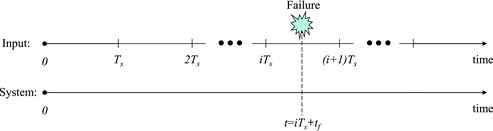
Figure 1 illustrates the two different viewpoints for a software failure described in Section 2.1. From the viewpoint of an input to the system, the failure occurs at some time point during the processing of the (i + 1)th input after successfully providing outputs for i consecutive inputs. From the viewpoint of the system operation, the failure occurs at some point of time after the system starts its operation.

Figure 1. Time relation for a failure from the input viewpoint and from the system operation viewpoint.

To distinguish between the two different viewpoints, two random variables are defined as follows:

• T_I: random variable indicating the time a failure occurs after an input is provided (0 ⩽ t < T_max)

• T_S: random variable indicating the time a failure occurs after the system starts its operation (t ⩾ 0)

where T_max is the maximum allowed execution time for an input.

From the two random variables, the following two probability density functions can be defined: (1) $$f_I\left(t\right)dt=P[t\le T_I<t+dt],$$(1) (2) $$f_S\left(t\right)dt=P[t\le T_S<t+dt],$$(2) wheref_I(t) is the failure probability density function for an input (0 ⩽ t < T_max) andf_S(t) is the failure probability density function for the system operation (t ⩾ 0).

Basically, whether a failure occurs or not for a given input is deterministic in the case of software. An input to the system can be understood as a result of sampling in a distribution of possible inputs, which is related to the plant condition at the time of sampling. The failure probability density functions, f_I(T) and f_s(T), depend on inputs and the sequence of inputs to the system, respectively. In summary, the failure probability density functions depend on the plant condition under consideration.

In a probabilistic analysis, the distribution of inputs that is weight-averaged over possible plant conditions with the consideration of the frequencies of the plant conditions needs to be used instead of a distribution of inputs for a specific plant condition. Therefore, the operational profile (various plant conditions with their frequencies considered) should be designed so that the input domain (the distribution of inputs) can be properly reflected to the operational profile.

From the two failure probability density functions, the following two cumulative failure probability density functions can be defined: (3) $$F_I\left(t\right)=P[T_I\le t]={\int }_0^t{f}_I\left(t^{\text{'}}\right)d{t}^{\text{'}},$$(3) (4) $$F_S\left(t\right)=P[T_s\le t]={\int }_0^t{f}_S\left(t^{\text{'}}\right)d{t}^{\text{'}},$$(4) where F_I(t) is the cumulative failure probability density function for an input (0 ⩽ t < T_max) and F_S(t) is the cumulative failure probability density function for the system operation (t ⩾ 0).

It should be noted that f_S(t) satisfies the condition (5) $${\int }_0^{\infty }{f}_S\left(t\right)=1.$$(5)

On the other hand, f_I(t) does not satisfy such a condition, because it is defined for a finite time duration as (6) $${\int }_0^{T_{max}}{f}_I\left(t\right)\le 1.$$(6)

The value of the left-hand side of Equation (6) is the failure probability required for the PSA of digital I&C systems, i.e., the failure probability for an input provided to the system with a relatively short time frame.

2.3. Relation between the two failure probability density functions

The failure probability of a system due to a software failure that occurs between time t and t + dt after successfully providing outputs corresponding to i consecutive inputs is given as (7) $$\begin{array}{ccc}\hfill f_S\left(t\right)dt& =& P[t\le T_S<t+dt]=P[t\le T_S<t+dt|T_S\hfill \\ & \ge & i{T}_{max}]·P[T_S\ge i{T}_{max}],\hfill \end{array}$$(7) where i is the number of consecutive inputs whose outputs are provided successfully (i = 0, 1, 2, …).

After successfully providing outputs for i consecutive inputs, the (i + 1)th input will be provided at time iT_max. After time iT_max, if it is assumed that the inputs prior to (i + 1)th input do not have effect on the (i + 1)th time interval, the conditional probability of a failure from the system operation viewpoint is determined by the probability of a failure from the viewpoint of an input with time parameter t − iT_max. Since the failure to generate the correct output for the (i + 1)th input also indicates the failure of the system, the failure probability from the system operation viewpoint after successful operation for the time iT_max is given as (8) $$\begin{array}{ccc}\hfill P[t& \le & T_S<t+dt|T_S\ge i{T}_{max}]\hfill \\ & =& P[t-i{T}_{max}\le T_I<t-i{T}_{max}+dt]\hfill \\ & =& f_I(t-i{T}_{max})dt\hfill \end{array}$$(8) for iT_max ⩽ t < (i + 1)T_max and i = 0, 1, 2, ….

The probability of successful operation for i consecutive inputs can be calculated as (9) $$\begin{array}{ccc}\hfill P[T_S\ge i{T}_{max}]& =& P[T_S\ge i{T}_{max}|T_S\ge (i-1)T_{max}]\hfill \\ & & ·P[T_S\ge (i-1)T_{max}].\hfill \end{array}$$(9)

The conditional probability of successful operation for i consecutive inputs after successful operation for (i − 1) consecutive inputs is the probability of successfully operating for a single input. In other words, it is the probability that no failure is experienced for the duration of T_max. Therefore, (10) $$\begin{array}{c}\hfill P[T_S\ge i{T}_{max}]=[1-F_I\left(T_{max}\right)]·P[T_S\ge (i-1)T_{max}].\end{array}$$(10)

From Equation (10), the probability of successful operation for i consecutive inputs is given as (11) $$P[T_S\ge i{T}_{max}]={[1-F_I\left(T_{max}\right)]}^i$$(11) for i = 0, 1, 2, ….

Taking Equations (8) and (11) into consideration, Equation (7) becomes (12) $$f_S\left(t\right)={[1-F_I\left(T_{max}\right)]}^i·f_I(t-i{T}_{max})$$(12) for iT_max ⩽ t < (i + 1)T_max and i = 0, 1, 2, ….

f_S(t) in Equation (12) satisfies Equation (5). The proof is provided in the Appendix 1. In a system that repeatedly receives inputs and provides outputs corresponding to these inputs, such as the safety-critical digital I&C systems (and therefore the software inside the systems), f_S(t) may be assumed to satisfy Equation (12).

Equation (12) can be applied to any f_I(t) as long as it satisfies Equation (6).

In deriving Equation (12), it is assumed that T_max is constant for each input for simplicity. If T_max varies depending on the input to the system, it is possible to derive equations in similar ways.

3. Applications

3.1. Exponential distribution – a special case

Exponential distributions are widely used for modeling the failure density function of a system or a software program. Examples of the application of exponential distribution to a software failure can be found in many research studies such as Musa et al. [11] and Malaiya et al. [16]. If f_I(t) is represented as an exponential distribution as (13) $$f_I\left(t\right)=\lambda e^{-\lambda t}$$(13) for 0 ⩽ t < T_max, where λ is the constant failure rate, and f_S(t) is written using Equation (10) as (14) $$\begin{array}{ccc}\hfill f_S\left(t\right)& =& {\left[e^{-\lambda T_{max}}\right]}^i·\lambda e^{-\lambda (t-i{T}_{max})}=e^{-\lambda i{T}_{max}}·\lambda e^{-\lambda (t-i{T}_{max})}\hfill \\ & =& \lambda e^{-\lambda t}\hfill \end{array}$$(14) for iT_max ⩽ t < (i + 1)T_max, then Equation (14) can be rewritten as (15) $$f_S\left(t\right)=\lambda e^{-\lambda t}$$(15) for t ⩾ 0.

A unique characteristic of the exponential distribution is that f_I(t) and f_S(t) have the same form. The advantage of this property is that if an exponential distribution is assumed for f_I(t), f_I(t) can be derived directly by determining f_S(t) based on the failure data from the operating history or software testing. It should also be noted that f_S(t) is independent of T_max.

f_S(t) in Equation (15) can be determined based on the failure data from the operating history or software testing, especially time-to-failure data. One of the most widely used methods for this purpose is the minimum mean square error (MMSE) estimation [17–19]. The time-to-failure data for a system or a software program is given as (16) $$t_1<t_2<\cdots <t_j<\cdots <t_n,$$(16) where j is the serial number for the time-to-failure data for a system or a software program (j = 1, 2, …, n), t_j is the jth time-to-failure data item, and n is the total number of time-to-failure data items.

In other words, when n failures have been observed after the operation of the system or software program for a long time, j is the identifier to indicate one of the n failures, especially jth failure.

For an exponential distribution, the mean square error function is given as (17) $$M\left(\lambda \right)=\sum _{j=1}^n{\left(1-e^{-\lambda t_j}-\frac{j}{n}\right)}^2,$$(17) where M(λ) is the mean square error function for an exponential distribution.

The best estimator for λ can be determined by finding the point where the derivative of the mean square error function equals 0. This is given as (18) $$\frac{dM}{d\lambda }={\left.2\sum _{j=1}^n{t}_j{e}^{-\lambda t_j}\left(1-e^{-2\lambda t_j}+\frac{j}{n}\right)\right|}_{\lambda =\widehat{\lambda }}=0,$$(18) where $\widehat{\lambda }$ is the best estimator for λ.

From Equation (18), it can be found that $\widehat{\lambda }$ satisfies the following relation: (19) $$\sum _{j=1}^n{t}_j{e}^{-\widehat{\lambda }{t}_j}\left(1-e^{-\widehat{\lambda }{t}_j}-\frac{j}{n}\right)=0.$$(19)

Therefore, $\widehat{\lambda }$ can be determined by finding the numerical solutions to Equation (19).

3.2. Weibull distribution

Weibull distributions are also widely used in modeling failures in which the failure rate varies as time changes. If f_I(t) is represented as a Weibull distribution by the equation (20) $$f_I\left(t\right)=\frac{\alpha }{\beta }{\left(\frac{t}{\beta }\right)}^{\alpha -1}{e}^{-{\left(\frac{t}{\beta }\right)}^{\alpha }}$$(20) for 0 ⩽ t < T_max, where α and β are constant coefficients, then f_S(t) is given by using Equation (12) as (21) $$\begin{array}{ccc}\hfill f_S\left(t\right)& =& {\left[e^{-{\left(\frac{T_{max}}{\beta }\right)}^{\alpha }}\right]}^i·\frac{\alpha }{\beta }\left(\frac{t-i{T}_{max}}{\beta }\right)e^{-{\left(\frac{t-i{T}_{max}}{\beta }\right)}^{\alpha }}\hfill \\ & =& \frac{\alpha }{\beta }\left(\frac{t-i{T}_{max}}{\beta }\right)e^{-{\left(\frac{t}{\beta }\right)}^{\alpha }}\hfill \end{array}$$(21) for iT_max ⩽ t < (i + 1)T_max and i = 0, 1, 2, ….

For a Weibull distribution, the mean square error function is given as (22) $$M(\alpha ,\beta )=\sum _{j=1}^n{\left(1-e^{-{\left(\frac{t_j}{\beta }\right)}^{\alpha }}-\frac{j}{n}\right)}^2,$$(22) where M(α, β) is the mean square error function for a Weibull distribution.

The best estimators for α and β can be determined by finding the point where the partial derivatives of the mean square error function equals 0. They are given as the solutions for the following simultaneous equations: (23) $$\begin{array}{ccc}\hfill \frac{\partial M}{\partial \alpha }& =& {\left.2\sum _{j=1}^n\left(1-e^{-{\left(\frac{t_j}{\beta }\right)}^{\alpha }}-\frac{j}{n}\right)e^{-{\left(\frac{t_j}{\beta }\right)}^{\alpha }}\log \frac{t_j}{\beta }{\left(\frac{t_j}{\beta }\right)}^{\alpha }\right|}_{\alpha =\widehat{a},\beta =\widehat{\beta }}\hfill \\ & =& 0,\hfill \end{array}$$(23) (24) $$\begin{array}{ccc}\hfill \frac{\partial M}{\partial \beta }& =& {\left.\frac{2\alpha }{\beta }\sum _{j=1}^n\left(1-e^{-{\left(\frac{t_j}{\beta }\right)}^{\alpha }}-\frac{j}{n}\right)e^{-{\left(\frac{t_j}{\beta }\right)}^{\alpha }}{\left(\frac{t_j}{\beta }\right)}^{\alpha }\right|}_{\alpha =\widehat{a},\beta =\widehat{\beta }}\hfill \\ & =& 0,\hfill \end{array}$$(24) where $\widehat{\alpha }$ is the best estimator for α and $\widehat{\beta }$ is the best estimator for β.

The best estimators, $\widehat{\alpha }$ and $\widehat{\beta }$, can be determined by finding the numerical solutions of Equations (23) and (24).

4. An example

Table 4 in NUREG/CR-6848 [20] provides 42 failure data items out of 500 inputs from the software testing of the Personnel entry/exit ACcess System (PACS). According to NUREG/CR-6848 [20], PACS is a simplified version of an automated personnel entry access system used to provide privileged physical access to rooms or buildings. Table 1 shows the failure data and related calculations. Software testing was performed for 500 inputs. It took 53,888 s and 42 failures were observed. From the viewpoint of system operation, the time to failure ranged from 105 to 4911 s, mostly in the range of 0–1000. From the viewpoint of system input, failures did not occur during the processing of 458 inputs, while failures occurred at sometime during the processing of each of the 42 inputs.

Table 1. Failure data in NUREG/CR-6848 [20] and related calculations.

Failure	Test	Cumulative		Time	Time to
number	case	time in	MTTF	to	failure
(r)	number	seconds (tr)	(r)	failure	(rearranged)
1	3	333	333.0	333	105
2	8	878	439.0	545	110
3	22	2345	781.7	1467	229
4	46	4894	1223.5	2549	243
5	77	8085	1617.0	3191	333
6	103	10,721	1786.8	2636	333
7	108	11,218	1602.6	497	396
8	113	11,855	1481.9	637	431
9	151	15,899	1766.6	4044	458
10	156	16,464	1646.4	565	497
11	160	16,922	1538.4	458	520
12	168	17,737	1478.1	815	529
13	172	18,168	1397.5	431	535
14	177	18697	1335.5	529	536
15	192	20,332	1355.5	1635	545
16	227	24,131	1508.2	3799	565
17	230	24,527	1442.8	396	593
18	236	25,120	1395.6	593	611
19	238	25,349	1334.2	229	637
20	246	26,242	1312.1	893	663
21	248	26,575	1265.5	333	681
22	257	27,403	1245.6	828	815
23	270	28,794	1251.9	1391	828
24	284	30,265	1261.0	1471	844
25	290	30,928	1237.1	663	893
26	295	31,464	1210.2	536	972
27	305	31,984	1184.6	520	1351
28	318	33,849	1208.9	1865	1391
29	319	33,959	1171.0	110	1467
30	340	36,175	1205.8	2216	1471
31	355	37,839	1220.6	1664	1635
32	360	38,374	1199.2	535	1664
33	361	38,479	1166.0	105	1826
34	369	39,323	1156.6	844	1865
35	371	39,566	1130.5	243	2216
36	380	40,538	1126.1	972	2549
37	396	42,364	1145.0	1826	2636
38	440	47,275	1244.1	4911	3191
39	446	47,886	1227.8	611	3321
40	476	51,207	1280.2	3321	3799
41	482	51,888	1265.6	681	4044
42	494	53,239	1267.6	1351	4911

MTTF: mean time to failure.

The 42 failure data items were obtained by testing the system against its operational profile. The probability of successfully providing outputs for an input is calculated to be 0.916 and, therefore, the failure probability for an input is calculated to be 0.084.

The failure data can be used to derive f_S(t). In this example, the derivation of f_I(t) from the software failure data by using Equation (12) is demonstrated. f_S(t) can also be determined by using Equation (12) if the failure data for inputs are provided.

For simplicity, it is assumed that an exponential distribution can be applied to describef_I(t). As shown in Equations (13) and (15), if f_I(t) follows an exponential distribution, f_S(t) also follows the same exponential distribution.

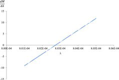
To obtain $\widehat{\lambda }$, the time-to-failure data are calculated from the 42 failure data items and rearranged so that Equation (16) is satisfied. Table 1 also shows the rearranged time-to-failure data. Figure 2 shows M(λ) as a function λ as given in Equation (17), and Figure 3 shows the derivative of M(λ) with respect to λ as given in Equation (18). The numerical solution for Equation (18) is given as the point in Figure 3 where the derivative of M(λ) with respect to λ becomes zero. Then, the best estimator for λ is given as (25) $$\widehat{\lambda }=8.0274\times {10}^{-4}{\mathrm{s}}^{-1}.$$(25)

Figure 2. Mean square error as a function of failure rate for the example failure data.

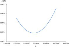
Figure 3. Derivative of mean square error function with respect to the failure rate for the example failure data.

Therefore, f_S(t) is given as (26) $$f_S\left(t\right)=\widehat{\lambda }{e}^{-\widehat{\lambda }t}$$(26) for t ⩾ 0.

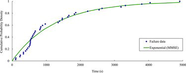
Figure 4 shows the failure data for the example system. F_S(t) is determined by the MMSE method.

Figure 4. Failure data and the cumulative failure probability density function for the system determined by the MMSE method.

As mentioned above, it is already shown in Equations (13) and (15) that in the case of exponential distributions, f_I(t) has the same form as f_S(t). In other words, the best estimator for λ in f_S(t) can also be used for f_I(t) as follows: (27) $$f_I\left(t\right)=\widehat{\lambda }{e}^{-\widehat{\lambda }t}$$(27) for 0 ⩽ t ⩽ T_max.

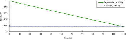
Figures 5 and 6 show f_I(t) and R_I(t) = 1 − F_I(t), respectively. In this example, f_I(t) and R_I(t) decrease monotonically for the defined duration as can be seen in Figures 5 and 6, respectively. Even though T_max for the example system is not specified in NUREG/CR-6848 [20], Figure 6 also provides the probability of successful operation for an input depending on T_max. For example, if T_max is given as 100 s, the success probability for an input is calculated to be 0.923, and the failure probability for the input is 0.077. As mentioned above, this failure probability is of interest in PSA of digital I&C systems. It should also be noted that the failure probabilities used in PSA of digital I&C systems will be much less than the one calculated for this example system. The time at which the reliability curve in Figure 6 meets the observed probability of successful operation (calculated from the software testing, i.e., 0.916) is calculated to be 109.3 s.

Figure 5. Failure probability density function for an input determined by the MMSE method.

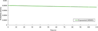
Figure 6. Reliability curve corresponding to the failure probability density function for an input determined by the MMSE method.

The method by which the failure data can be used to determine f_S(t), and eventually f_I(t), by using Equation (12) is demonstrated. As mentioned above, Equation (12) can also be used to derive f_I(t) from f_S(t).

It should be noted that even though a non-exponential distribution is assumed for f_I(t), the procedure to determine f_I(t) from the failure data will be similar to the one described above for the exponential distribution assumption. For example, when a Weibull distribution is assumed, f_S(t) can be defined as shown in Equation (21), and the best estimates for the two coefficients, α and β, can be determined by applying the MMSE method as shown in Equations (23) and (24).

The best estimates for the two coefficients can be used to determine f_I(t), as shown in Equation (20).

5. Conclusions

When the software reliability of a digital system is estimated based on the failure data from the operating history or software testing (especially statistical software testing), the failure data are generally collected from the viewpoint of the system operation. However, for conducting PSA of the digital I&C system, the failure probability with respect to an input to the system is required. Thus, there exist two viewpoints for a system failure: one with respect to the system operation and the other with respect to an input to the system. Therefore, it is important to clearly distinguish between the two different viewpoints and obtain the correct relation between them.

In this paper, two failure probability density functions for the two viewpoints were defined, and the relation between the two failure probability density functions was derived and presented. Based on the two failure probability density functions, it was also shown how the failure probability density function from the system operation viewpoint can be derived from the failure probability density function from the viewpoint with respect to an input to the system. This was illustrated using two example distributions, the exponential distribution and the Weibull distribution.

The derivation of the failure probability density function for an input from the software testing results was also demonstrated. This derivation was based on the assumption that the failure probability density function for an input follows an exponential distribution. In addition, the failure probability density function for an input was derived in a similar way when a non-exponential distribution was assumed.

The relation between the failure probability density function from the system operation viewpoint and that from the viewpoint of an input to the system, presented in this paper, not only helps us derive one from the other but also extend our understanding of how statistical software testing can be used to estimate or demonstrate the reliability of the software.

Additional information

Funding

This research was supported by Chung-Ang University Research Grants received in 2013; Nuclear Research & Development Program of the National Research Foundation, with funding by the Korean government's Ministry of Science, ICT and Future Planning [grant number 2012M2A8A4025991].

Appendix 1

The proof that the failure probability density function for the system provided in Equation (12) satisfies Equation (5) is provided in this appendix.

The left-hand side of Equation (5) is given as (A1) $$\begin{array}{ccc}& & {\int }_0^{\infty }{f}_S\left(t\right)dt\hfill \\ & & ={\int }_0^{\infty }{[1-F_I\left(T_s\right)]}^i·f_I(t-i{T}_s)dt\hfill \\ & & ={\int }_0^{T_s}{f}_I\left(t\right)dt+[1-F_I\left(T_s\right)]{\int }_{T_s}^{2T_s}{f}_I(t-T_s)·dt\hfill \\ & & +{[1-F_I\left(T_s\right)]}^2{\int }_{2T_s}^{3T_s}{f}_I(t-2T_s)dt+\cdots \hfill \\ & & ={\int }_0^{T_s}{f}_I\left(t\right)dt+[1-F_I\left(T_s\right)]{\int }_0^{T_s}{f}_I\left(t\right)dt\hfill \\ & & +{[1-F_I\left(T_s\right)]}^2{\int }_0^{T_s}{f}_I\left(t\right)dt+\cdots \hfill \\ & & =F_I\left(T_s\right)+[1-F_I\left(T_s\right)]·F_I\left(T_s\right)\hfill \\ & & +{[1-F_I\left(T_s\right)]}^2·F_I\left(T_s\right)+\cdots .\hfill \end{array}$$(A1)

By substituting k = 1 − F_I(T_s), where 0 ⩽ k < 1, Equation (A1) becomes (A2) $$\begin{array}{ccc}& & {\int }_0^{\infty }{f}_S\left(t\right)dt\hfill \\ & & =(1-k)+k(1-k)+k^2(1-k)+\cdots \hfill \\ & & =(1-k)(1+k+k^2+\cdots ).\hfill \end{array}$$(A2)

Substituting the infinite series part in Equation (A2) with S yields (A3) $$S=1+k+k^2+\cdots .$$(A3)

Multiplying both sides of Equation (A3) by k, we have (A4) $$kS=k+k^2+k^3+\cdots .$$(A4)

Subtracting Equation (A4) from Equation (A3), we have (A5) $$(1-k)S=1.$$(A5)

From Equations (A3)–(A5), the infinite series part in Equation (A2) is given as (A6) $$S=\frac{1}{1-k}.$$(A6) Therefore, Equation (A2) becomes (A7) $${\int }_0^{\infty }{f}_S\left(t\right)dt=(1-k)\frac{1}{1-k}=1.$$(A7)

Equation (A7) proves that the failure probability density function provided in Equation (12) satisfies Equation (5).

References

- Lu L, Jiang J. Probabilistic safety assessment for instrumentation and control systems in nuclear power plants: an overview. J Nucl Sci Technol. 2004;41(3):323–330.
- Kang HG, Kim MC, Lee SJ, Lee HJ, Eom HS, Choi JG, Jang S-C. An overview of risk quantification issues for digitalized nuclear power plants using a static fault tree. Nucl Eng Technol. 2009;41(6):849–858.
- Authen S, Holmberg J-E. Reliability analysis of digital systems in a probabilistic risk analysis for nuclear power plants. Nucl Eng Technol. 2012;44(5):471–482.
- Kang HG, Sung T. An analysis of safety-critical digital systems for risk-informed design. Reliab Eng Syst Saf. 2002;78:307–314.
- STD-729-1991. Standard glossary of software engineering terminology. New York (NY): The Institute of Electrical and Electronics Engineers; 1991.
- Lyu MR. Handbook of software reliability engineering. Hightstown (NJ): McGraw-Hill, Inc.; 1996.
- Chu T-L, Yue M, Martinez-Guridi G, Lehner J. Review of quantitative software reliability methods. BNL-94047-2010. Upton (NY): Brookhaven National Laboratory; 2010.
- Myers GJ. The art of software testing. New York (NY): Wiley; 1979.
- IEEE Std 829-1998. IEEE standard for software test documentation. New York (NY): The Institute of Electrical and Electronics Engineers; 1998.
- Currit PA, Dyer M, Mills HD. Certifying the reliability of software. IEEE Trans Softw Eng. 1986;SE-12(1):3–11.
- Musa JD, Iannino A, Okumoto K. Software reliability: measurement prediction application. New York (NY): McGraw-Hill; 1987.
- Chillarege R. Software testing best practices, IBM Research Technical Report RC 21457. Yorktown Heights (NY): ( IBM Thomas J. Watson Research Center; 1999.
- Banks D, Dashiell W, Gallagher L, Hagwood C, Kacker R, Rosenthal L. Software testing by statistical methods – preliminary success estimates for approaches based on binomial models, coverage designs, mutation testing, and usage models. Gaithersburg (MD): National Institute of Standards and Technology; 1998.
- Jelinski Z, Moranda PB. Software reliability research, In: Freiberger W, editor. Statistical computer performance evaluation. New York (NY): Academic Press; 1972. p. 465–484.
- Goel AL, Okumoto K. Time-dependent error-detection rate model for software reliability and other performance measures. IEEE Trans Reliab. 1979;R-28(3):206–211.
- Malaiya YK, von Mayrhauser A, Srimani PK. An examination of fault exposure ratio. IEEE Trans Softw Eng. 1993;19(11):1087–1094.
- Bibby J, Toutenburg H. Prediction and improved estimation in linear models. New York (NY): Wiley; 1977.
- Kay SM. Fundamentals of statistical signal processing: estimation theory. Englewood Cliffs (NJ): Prentice-Hall PTR; 1993.
- Moon TK, Stirling WC. Mathematical methods and algorithms for signal processing. Upper Saddle River (NJ): Prentice Hall; 2000.
- Smidts C, Li M. Validation of a methodology for assessing software quality (NUREG/CR-6848). Washington (DC): United States Nuclear Regulatory Commission; 2004.