Development of a three-dimensional magnetohydrodynamics code for electromagnetic pumps

Abstract

Annular linear induction pumps (ALIPs) are one of the electromagnetic (EM) pumps, which drive liquid metal using EM force, for fast reactors and have been developed in many countries. An ALIP mainly consists of multiple coils, iron cores and an annular flow channel. We have calculated the developed pressure of ALIPs using a two-dimensional magnetohydrodynamics (MHD) code. There are some reports in which pressure drop and fluctuation were observed in EM pump operations near the top of the pressure and flow rate relation (P–Q) curve. For fear of this phenomenon, the EM pump design is sometimes too conservative. To simulate the pressure drop and fluctuation occurrence conditions, we have developed a new three-dimensional (3D) MHD code. Clarification of this condition and its phenomena in the sodium flow will enable design of a new structure or determination of operation conditions that preclude this pressure drop and fluctuation and, thereby, achieve high efficiency. In this paper, the model of our new 3D MHD code, the accuracy of the code, simulation results focusing on pressure drop and fluctuation by radial and circumferential vortices are reported.

Keywords:

• electromagnetic pump
• MHD
• stability
• analysis
• liquid metal
• sodium-cooled fast reactor

1. Introduction

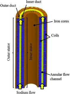
Electromagnetic (EM) pumps, which drive liquid metal using EM force, for fast reactors have been developed [1,2]. EM pumps are static equipment that have no mechanical moving parts and circulate sodium using EM force, and are advantageous in terms of reliability and maintainability. An annular linear induction pump (ALIP) is one of the EM pumps and is suitable for increasing capacity. An overview of an ALIP is shown in Figure 1. An ALIP has a simple structure, which mainly consists of multiple coils operated with three-phase current, iron cores, and an annular flow channel.

Figure 1. Bird's-eye view of an EM pump.

In general, performance of an EM pump is described by the pressure and flow rate relation (P–Q) curve. Reducing the flow rate and setting the operation point near the peak of the P–Q curve sometimes bring about developed pressure drops and fluctuations [1]. These fluctuations were reported as instability by Gailitis et al. [3], Kirillov et al. [4], and Araseki et al. [5]. The instability was characterized by vortices, which were initiated by circumferential non-uniformity of sodium velocity and/or magnetic field, in the sodium flow. According to Gailitis, the stable/unstable boundary was defined as the condition where the overall magnetic Reynolds number, Rm, times the slip velocity, s, is higher than unity. Mechanical pumps connected in parallel sometimes suffer this type of instability as well.

We have calculated the developed pressure of ALIPs using a two-dimensional – radially and axially – MHD code. The code simulated the developed pressure with high accuracy for normal operations. When the flow rate is decreased and this type of instability occurs, however, the accuracy deteriorates since this type of instability could not be simulated properly. Therefore, the pump has been designed with the condition that Rm × s is smaller than unity, which is sometimes too conservative and requires higher manufacturing cost.

To overcome this problem, we have developed a new three-dimensional (3D) MHD code to simulate this type of instability to evaluate the developed pressure with high accuracy. This code should treat EM force and sodium flow simultaneously, and requires large-scale calculations in a reasonable time.

Section 2 of this paper presents our model of the 3D MHD code coupling fluid dynamics simulation with magnetic field simulation. Section 3 shows the simulation results of the developed pressure for 160 m³/min ALIP experiments. The simulated developed pressures are compared with experimental results. In Section 4, the simulation of the pressure drop and fluctuation is shown. Vortices in radial and circumferential directions are observed in the sodium flow for certain operation conditions. Conclusions are given in Section 5.

2. MHD code

2.1. Basic equations and boundary conditions

The structure of our 3D MHD code is shown in Figure 2. The code consists of a magnetic field calculation part and a fluid dynamics calculation part, both of which are weakly coupled. The magnetic field calculation part has been made in-house, and the fluid dynamics part exploits commercial computational fluid dynamics (CFD) software, STAR-CD^TM. The fluid velocity in the annular flow channel is calculated by STAR-CD^TM and transferred to the magnetic field calculation part to calculate the EM force. The EM force obtained by the magnetic field calculation is transferred back to the CFD. The use of widely used commercial CFD codes such as STAR-CD^TM gives flexible options for various turbulence models depending on the fluid conditions of interest.

Figure 2. 3D MHD code algorithm.

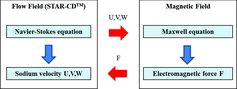
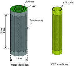
The fluid calculations are done in the annular flow channel only while the magnetic calculation includes the pump casing, air, iron cores, coils, and inner and outer ducts, in addition to sodium. Therefore, both calculations can share meshes in the annular flow channel and no interpolation is required.

We use the magnetic field equations in the A–ϕ formulation, which are given by (1) $$\begin{array}{ccc}& & \nabla \times \left(\frac{1}{\mu }\nabla \times \mathit{A}\right)\hfill \\ & & ={\mathit{I}}_0+\sigma \left\{-\frac{\partial \mathit{A}}{\partial t}-\nabla \phi +\mathit{u}\times (\nabla \times \mathit{A})\right\}\hfill \end{array}$$(1) and (2) $$\sigma \left\{-\frac{\partial (\nabla ·\mathit{A})}{\partial t}-\nabla \phi +\nabla ·[\mathit{u}\times (\nabla \times \mathit{A})]\right\}=0.$$(2)

These equations are discretized and solved by the edge-based finite element method. The edge-based finite element method is advantageous over the usual node-based finite element method in the following points:

1. Discretization automatically satisfies the boundary conditions of magnetic fields between permeability materials.

2. Unknown variables are generally smaller in number.

As to this method, we refer you to [6]. An element coefficient matrix using the edge-based hexahedral finite element method is shown below. (3) $$\begin{array}{ccc}\hfill & & \left[\begin{array}{cccccccc}{G}_{A1A1}& G_{A1A2}& \cdots & G_{A1A12}& G_{A1\phi 1}& G_{A1\phi 2}& \cdots & G_{A1\phi 8}\\ G_{A2A1}& G_{A2A2}& \cdots & G_{A2A12}& G_{A2\phi 1}& G_{A2\phi 2}& \cdots & G_{A2\phi 8}\\ ⋮& ⋮& \ddots & ⋮& ⋮& ⋮& \cdots & ⋮\\ G_{A12A1}& G_{A12A2}& \cdots & G_{A12A12}& G_{A12\phi 1}& G_{A12\phi 4}& \cdots & G_{A12\phi 8}\\ G_{\phi 1A1}& G_{\phi 1A2}& \cdots & G_{\phi 1A12}& G_{\phi 1\phi 1}& G_{\phi 1\phi 2}& \cdots & G_{\phi 1\phi 8}\\ G_{\phi 2A1}& G_{\phi 2A2}& \cdots & G_{\phi 2A12}& G_{\phi 2\phi 1}& G_{\phi 2\phi 2}& \cdots & G_{\phi 2\phi 8}\\ ⋮& ⋮& \cdots & ⋮& ⋮& ⋮& \ddots & ⋮\\ G_{\phi 8A1}& G_{\phi 8A2}& \cdots & G_{\phi 8A12}& G_{\phi 8\phi 1}& G_{\phi 8\phi 2}& \cdots & G_{\phi 8\phi 8}\end{array}\right]\hfill \\ \hfill & & \times \left[\begin{array}{c}{A}_1\\ A_2\\ ⋮\\ A_{12}\\ {\phi }_1\\ {\phi }_2\\ ⋮\\ {\phi }_8\end{array}\right]=\left[\begin{array}{c}{F}_{A1}\\ F_{A2}\\ ⋮\\ F_{A12}\\ F_{\phi 1}\\ F_{\phi 2}\\ ⋮\\ F_{\phi 8}\end{array}\right].\hfill \end{array}$$(3) where $$\begin{array}{ccc}\hfill G_{A_k{A}_{k^{\text{'}}}}& =& \frac{1}{\mu }{\int }_{V_e}\{(\nabla \times {\mathbf{N}}_k)·(\nabla \times {\mathbf{N}}_{k^{\text{'}}})\}\left|J\right|\mathrm{d}{V}_e\hfill \\ & & +\frac{\sigma }{\Delta t}{\int }_{V_e}\left\{\left({\mathbf{N}}_k\right)·\left({\mathbf{N}}_{k^{\text{'}}}\right)\right\}\left|J\right|\mathrm{d}{V}_e\hfill \\ & & -\sigma {\int }_{V_e}[\left({\mathbf{N}}_k\right)·\{\left(\sum _{j=1}^8\left(\nabla N_j\right)u_j\right){(\nabla \times {\mathbf{N}}_{k^{\text{'}}})}_z\hfill \\ & & -\left(\sum _{i=1}^8\left(\nabla N_j\right)u_j\right){(\nabla \times {\mathbf{N}}_{k^{\text{'}}})}_y\left\}\right]\left|J\right|\mathrm{d}{V}_e,\hfill \\ \hfill G_{A_k{\phi }_i}& =& \sigma {\int }_{V_e}\left\{\left({\mathbf{N}}_k\right)·\left(\nabla N_i\right)\right\}\left|J\right|\mathrm{d}{V}_e,\hfill \\ \hfill G_{{\phi }_i{A}_k}& =& \frac{\sigma }{\Delta t}{\int }_{V_e}\{\left(\nabla N_i\right)·\left({\mathbf{N}}_k\right)\}\left|J\right|\mathrm{d}{V}_e\hfill \\ & & -\sigma {\int }_{V_e}\left[{\left(\nabla N_i\right)}_x\right\{\left(\sum _{j=1}^8\left(\nabla N_j\right)u_j\right)(\nabla \times {\mathbf{N}}_{k^{\text{'}}})\hfill \\ & & -\left(\sum _{j=1}^8\left(\nabla N_j\right)u_j\right)(\nabla \times {\mathbf{N}}_{k^{\text{'}}})\left\}\right]\left|J\right|\mathrm{d}{V}_e,\hfill \\ \hfill G_{{\phi }_i{\phi }_{i^{\text{'}}}}& =& \sigma {\int }_{V_e}\{\left(\nabla N_i\right)·\left(\nabla N_{i^{\text{'}}}\right)\}\left|J\right|\mathrm{d}{V}_e,\hfill \\ \hfill F_{A_k}& =& {\int }_{V_e}\{\left({\mathbf{N}}_k\right)·I_0\}\left|J\right|\mathrm{d}{V}_e\hfill \\ & & +\frac{\sigma }{\Delta t}{\int }_{V_e}\sum _{k^{\text{'}}=1}^{12}\{\left({\mathbf{N}}_k\right)·\left({\mathbf{N}}_{k^{\text{'}}}\right)\}{A}_{k^{\text{'}}}^t\left|J\right|\mathrm{d}{V}_e,\hfill \\ \hfill F_{{\phi }_i}& =& \frac{\sigma }{\Delta t}{\int }_{V_e}\left\{\sum _{k=1}^{12}\{\left(\nabla N_i\right)·\left({\mathbf{N}}_k\right)\}{A}_k^t\right\}\left|J\right|\mathrm{d}{V}_e,\hfill \\ \hfill {\mathit{A}}_k& =& \left\{A_k^{t+\Delta t}\right\},\hfill \end{array}$$and $$\begin{array}{c}\hfill {\phi }_i=\left\{{\phi }_i^{t+1}\right\}.\end{array}$$

Element coefficient matrices made for various materials are added to construct the global coefficient matrix. In solving the discretized simultaneous global coefficient matrix, BiCGSTab with the Jacobi pre-conditioner is used. The solvers we have used have been developed by a Japanese National Project and released in a sparse matrix solver package, Library of Iterative Solvers (LIS). Once the magnetic flux density and the eddy current density in sodium are calculated using vector and scalar potentials, A and ϕ, the Lorentz force at every fluid cell is given by (4) $$F_{\mathrm{mag}}=I\times B,$$(4) which is transferred to the CFD part and used as external forces in the fluid calculation.

The boundary conditions are set as follows:

• For magnetic field calculation, the boundary is set sufficiently far from the fluid region and Dirichlet conditions are given.

• For the fluid calculation, there is no specific limitation for selection of boundary conditions. In the simulations presented hereafter, for example, the normal inlet flow velocity condition, non-slip on the wall, and free outlet conditions supplied by the CFD code are used.

3. Code validation using ETEC experimental results

3.1. ETEC 160 m³/min specification

A large EM pump experiment at Energy Technology and Engineering Center (ETEC) was held in 2001 [1]. This EM pump was a double stator type. The design specifications of the EM pump are shown in Table 1 [1]. The developed pressure is 0.25 MPa at a rated flow rate of 160 m³/min. The magnetic Reynolds number is 1.06. This EM pump has 168 coils; each coil has 16 turns except the last set of coils to moderate the spatial change of the magnetic field near the end of the pump.

Table 1. ETEC 160 m³/min specifications.

Items	Specification
Flow rate	160 m^3/min
Developed pressure (pump head)	0.25 MPa
Sodium temperature	335 °C
Design specification
Input power	1680 kW
Terminal voltage	884 A
Frequency	20 Hz
Rm	6.42
Slip	0.16
Rm × slip	1.06
Number of poles	14
Flow gap	77 mm
Flow velocity	10.4 m/s
Number of coils	84 × 2
Outer diameter of casing	1900 mm

We calculated the developed pressures of this EM pump for various operation conditions using the new 3D MHD code and compared the numerical and experimental results for validation.

3.2. Developed pressure simulation

3.2.1. Models and conditions

The simulation conditions are shown in Table 2. The mesh we used is presented in Figure 3. Parameters are coil currents, operation frequencies and flow rates. The coil currents for the simulation input were set the same as those measured in the experiments.

Table 2. Simulation conditions.

No.	1	2	3	4	5	6	7	8	9	10
Flow rate (m^3/min)	141	151	156	159	164	172	73	117	126	137
Inlet velocity (m/s)	9.0	9.7	10.0	10.2	10.5	11.0	4.7	7.5	8.1	8.8
Frequency (Hz)	20.4	20.4	20.4	20.4	20.4	20.4	15.9	15.9	16.0	16.1
Average coil currents (A)	344	333	323	313	298	282	341	302	281	253

Figure 3. ETEC 160 m³/min mesh.

Simulations were conducted in the following steps:

1. Steady-state fluid calculation is conducted for the annular flow channel without EM pump operation to obtain the steady-state flow for the initial condition. Inlet fluid velocity is used for the boundary condition.

2. Coupled simulations are done with EM pump operation with the same inlet fluid velocity.

3. Calculation is continued until the time-averaged developed pressure stabilizes.

The time until the developed pressure stabilizes is about 0.2 sec. The time step was chosen so that it is sufficiently small compared with the coil current variation, i.e. the operation frequency. After several trial calculations, the time step was determined as a 1/200 sine-wave period.

The EM pump operation frequencies are 20.4 and 16 Hz. The flow rates and coil currents in simulations were varied in accordance with the experiments. The flow velocity distribution is uniform in the circumferential direction. The obtained P–Q curve was compared with experiments.

3.2.2. Simulation results

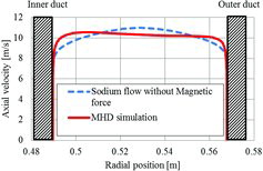
Figure 4 shows the pressure contour in the center of the annular flow channel at an operation frequency of 20.4 Hz and a flow rate of 160 m³/min. The pressure increased as the sodium flowed from the inlet to the outlet. The developed pressure was calculated to be 0.29 MPa in this case. Figure 5 shows that the flow velocity distribution becomes broad since EM force acts on the sodium near the channel wall due to the skin effect. In this way, the sodium flow could be clearly visualized using the 3D MHD code.

Figure 4. Pressure contour (159 m³/min, 20.4 Hz, 0.5 sec).

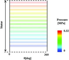
Figure 5. Flow velocity distribution at pump outlet (159 m³/min, 20.4 Hz, 0.5 sec).

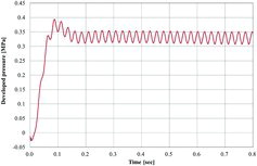
The transient variation of the developed pressure, ΔP, is shown in Figure 6. The horizontal axis is time and the vertical axis is developed pressure. The developed pressure developed from 0 to 0.15 sec, and then periodical fluctuations in the double-supply-frequency (DSF). This DSF was observed in various experiments and simulations [7]. The experimental and simulated developed pressures versus the sodium flow rates, P–Q curves, are shown in Figure 7. The error bar shows the pressure fluctuation in the experiment. In plotting this figure, the developed pressure was averaged where the periodic fluctuation became stable. The peaks of simulated and experimental developed pressures on the P–Q curves were in good agreement with an error smaller than 6% at a rated flow rate.

Figure 6. Transient of the developed pressure (159 m³/min, 20.4 Hz).

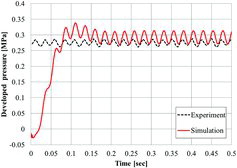
Figure 7. P–Q characteristics: simulations and experiments.

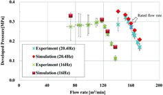
However, the simulations and experiments quite disagreed in a range where the flow rate was lower than the peak of the P–Q curve. In the simulation, the developed pressure continued to rise as the flow rate decreased, while experimental results showed a drop in the developed pressure. These phenomena are commonly known as instability. Detailed simulations and discussions with regard to the pressure drop and fluctuation are presented in the following section.

4. Pressure drops and fluctuations by sodium vortices

4.1. Simulation conditions

Low-frequency (LF) pressure pulsation is considered as one of the magnetohydrodynamic instabilities. This was reported by Araseki et al. [5] and other researchers [3,4]. According to [5], this instability is initiated by circumferential non-uniformity in the sodium flow velocity and/or of the magnetic fields and ends up with vortices in the sodium flow. In this section, we present these phenomena with the 3D MHD code. The circumferential non-uniform distribution is given to the inlet flow velocity as a boundary condition in the form of a sine-wave function. An example of flow velocity distribution is shown in Figure 8. The horizontal axis denotes the circumferential direction and the vertical axis denotes the axial sodium velocity. To evaluate the effect of inlet velocity variation, the peak of the flow speed distribution is varied.

Figure 8. Circumferential non-uniformity of flow velocity in inlet boundary condition.

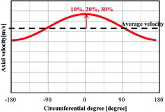
Table 3 summarizes the simulation conditions. First, stability at the rated flow rate, 150 m³/min, was confirmed. Then the flow rate was decreased below the peak of the P–Q curve – 140 m³/min – and the peak values of the inlet flow distribution were varied to clarify the pressure drop boundary.

Table 3. Simulation conditions.

Flow rate (m^3/min)	141	141	141	141	151
Inlet velocity (m/s)	9.0	9.0	9.0	9.0	9.7
Frequency (Hz)	20.4	20.4	20.4	20.4	20.4
Rm × s	1.6	1.6	1.6	1.6	1.4
Average coil currents (A)	300	300	300	300	333
Non-uniformity (%)	0	10	20	30	10

4.2. Simulation results

First, we examined prospectively stable cases with a flow rate of 150 m³/min. We changed the variation of inlet velocity distribution by up to 10% and examined the transient response of the developed pressure. This velocity distribution was a parameter for sensitivity simulations. The axial velocity in the center of the flow channel at 0.98 sec is shown in Figure 9 and the developed pressure with time is shown in Figure 10. During early stages of the simulation, the developed pressure fluctuated periodically and was constant. It should be noted that this EM pump operation is numerically and experimentally stable even at Rm × s = 1.4 although Rm × s is sometimes said to be smaller than 1 for the stable operation of EM pumps.

Figure 9. Contour of the flow velocity (151 m³/min, Rm × s = 1.4, non-uniformity 10%).

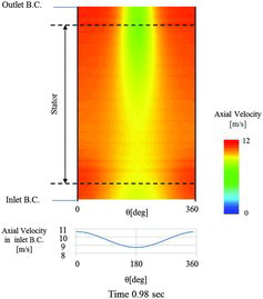
Figure 10. Transient of developed pressure (151 m³/min, Rm × s = 1.4, non-uniformity 10%).

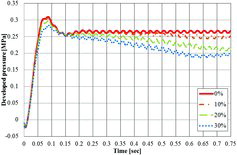
Next, we examined the lower flow rate case. Figure 11 shows the transient response of the developed pressure for a flow rate of 140 m³/min and with inlet peak variations of 0%, 10%, 20%, and 30%. It was observed that the developed pressure drops more as the non-uniformity becomes bigger.

Figure 11. Transient of developed pressure with non-uniformity (141 m³/min, Rm × s = 1.4).

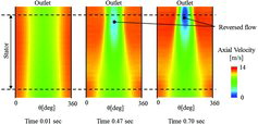
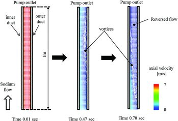
Figure 12 shows contours of the flow velocity in the center of the annular flow channel for the 30% non-uniform case. During the passage of time, reversed flow of the sodium was observed and strong vortices developed toward the end of the pump. These types of vortices would be the same phenomena observed by Araseki et al. [5] under a condition that Rm × s was greater than unity.

Figure 12. Contours of axial flow velocity (141 m³/min, Rm × s = 1.6, non-uniformity 30%).

Looking into this phenomenon in more detail, vortices in the radial direction were also observed. The flow vector in relevant r–z plane is presented in Figure 13. Vortices developed in the boundary region near the outer duct first and, then, spread toward the inner direction. The appearance of these vortices near the outer duct is considered to be due to radial non-uniformity of the magnetic field and velocity. The magnetic field in the sodium and the duct decreased due to the skin effect and the field was non-uniform in the radial direction. As the currents of the outer and inner coils were the same, the magnetic field near the outer duct is likely to be smaller than that near the inner duct. We consider that the vortices develop more easily in regions where the flow velocity is lower – i.e. the slip is bigger – and the magnetic field is weaker.

Figure 13. The flow vectors in r–z plane (141 m³/min, Rm × s = 1.6, non-uniformity 30%).

5. Conclusion

In this paper, the summary of our newly developed 3D MHD code and numerical results focusing on developed pressure fluctuation and drop triggered by the distributed inlet flow were presented. 3D simulations provide a clearer illustration of the vortices in the sodium flow. The conclusions obtained are as follows:

1. Simulated and experimental developed pressures at the rated flow rate were in very good agreement. The error was smaller than 6%.

2. Periodical fluctuations in the developed pressure were observed at the DSF.

3. Without circumferential inlet velocity distribution, the EM pump operation was stable even at Rm × s = 1.4.

4. Given a circumferential non-uniformity for inlet fluid velocity distribution, vortices were observed in the sodium flow at the end of the EM pump. Here Rm × s was 1.6.

5. Vortices in the sodium flow appeared first near the outer wall in the radial direction, spread into the inner direction, and, then, grew to the circumferential direction.

6. Conditions of pressure drop by the vortices were presented. Our new 3D MHD code would make possible a more proper EM pump design.

We would be able to change the turbulent model into other models and evaluate the influence of them on the initiation of these vortices using the 3D MHD code.

Nomenclature

B	=	magnetic field
I0	=	coil current
I	=	induced current
u	=	sodium velocity vector
Fmag	=	magnetic force
Q	=	flow rate
V	=	average sodium velocity
Vs	=	synchronous sodium velocity
A	=	magnetic vector potential
f	=	current frequency
σ	=	electric conductivity
μ	=	magnetic permeability
ρ	=	fluid density
ϕ	=	electric scholar potential
ω	=	angular frequency, ω = 2πf
Nk	=	shape function in edge
Ni	=	shape function in node
s	=	slip = (Vs − V)/Vs
Rm	=	magnetic Reynolds number
J	=	Jacobian
Δt	=	time step

Acknowledgements

The authors wish to thank Prof. Hoashi for helpful comments on coding and preparation of this article.

References

- Ota H, Katsuki K, Funato M, Taguchi J, Fanning AW, Doi Y, Nibe N, Ueta M, Inagaki T. Development of 160 m3/min large capacity sodium-immersed self-cooled electromagnetic pump. J Nucl Sci Technol. 2004;41:511–523.
- Kittaka D, Asada T, Aizawa R, Komai M, Oota H. Development of electromagnetic pump and electromagnetic flow meter for 4S. American Nuclear Society: 2011 Winter Meeting; 2011 Oct. 30–Nov. 3; Washington, DC.
- Gailitis A, Lielausis O. Instability of homogeneous velocity distribution in an induction-type MHD machine. Magnitnaya Gidrodinamika; 1975;1:87–101.
- Kirillov IR, Ogorodnikov AP, Ostapenko VP. Experimental investigation of flow nonuniformity in a cylindrical linear induction pump. Magnitnaya Gidrodinamika; 1980;2:107–113.
- Araseki H, Kirillov IR, Preslitsky GV, Ogorodnikov AP. Magnetohydrodynamic instability in annular linear induction pump. Part I. Experiment and numerical analysis. J Nucl Eng Des. 2004;227:29–50.
- Takahashi N. Three dimensional finite element method. Denki-gakkai; 2006;40–54.
- Araseki H, Kirillov IR, Preslitsky GV, Ogorodnikov AP. Double-supply-frequency pressure pulsation in annular linear induction pump. Part I. Measurement and numerical analysis. J Nucl Eng Des. 2000;195:85–100.