An improved Feynman-α analysis with a moving–bunching technique

ABSTRACT

The bunching technique has been widely utilized in Feynman-α neutron correlation analysis to synthesize neutron counts within longer gate widths by bunching time-sequence neutron counts stored in multichannel scaler channels. An alternative technique referred to as “moving–bunching technique” was proposed to reduce a statistical scatter of variance-to-mean ratio of neutron counts. The conventional bunching technique has no overlap of adjacent bunches, while the present technique makes adjacent bunches overlap as long as possible similarly to the moving average technique. A Feynman-α experiment was performed in the UTR-KINKI, to confirm the advantage of the proposed bunching technique. When a neutron detector was placed far from the core, a Feynman-α analysis with the conventional bunching technique led to a scattered variance-to-mean ratio from which the prompt-neutron decay constant was never determinable. However, another analysis with the proposed technique remarkably reduced the above scatter and enabled the determination of the decay constant. For a neutron detector close to the core, the proposed technique also reduced statistical error of the decay constant.

Keywords:

• UTR
• nuclear reactor
• Feynman-α
• analysis
• reactor kinetics
• subcriticality

1. Introduction

The Feynman-α (variance-to-mean ratio) method [1] has been frequently employed to determine kinetic parameters of various nuclear reactor systems. In the earlier Feynman-α experiments, neutron counts within a specified time interval (gate width) were continuously registered by the use of a multichannel scaler (MCS). The bunching technique [2] has been employed to synthesize the count data within longer time widths than the gate width of the MCS. On the basis of the time-sequence count data generated by the synthesis, the statistical indication Y was calculated in the longer gate-width range. The indication Y is defined as the variance-to-mean ratio of the neutron counts minus 1. Provided that the probability of neutron detection follows the Poisson distribution, the indication Y should be zero. The correlation between detection events gives the deviation of the indication from zero. The Feynman-α method determines the prompt-neutron decay constant from the gate-width dependence of the Y. In the recent Feynman-α experiments, arriving times of neutrons at a neutron detector are continuously registered as digital data in a memory module, and the arriving time data are read by personal computer [3,4]. In this case, neutron counts within a time interval also are generated from the arriving time data and then the time-sequence count data within longer intervals are synthesized by the bunching technique. The Feynman-α analysis mentioned above has a serious problem as follows. When a neutron detector is placed far from core, the Feynman-α method suffers from a statistical scatter of the Y and consequently the prompt-neutron decay constant can be never determined.

In this study, an alternative bunching technique referred to as “moving–bunching technique” is proposed to reduce the above scatter of the Y and the statistical error of the decay constant. The further objective of this study is to demonstrate experimentally the advantage of the proposed technique. To achieve this goal, we performed a Feynman-α experiment in the UTR-KINKI and acquired time-sequence count data of neutron detectors, which were placed at various positions of the reactor. In this paper, the conventional and the present bunching techniques are described in Section 2, the reactor configuration and the experimental setups in Section 3, the discussion of the experimental results in Section 4, and the conclusion of this study in Section 5.

2. Bunching technique for Feynman-α analysis

2.1. Conventional bunching technique

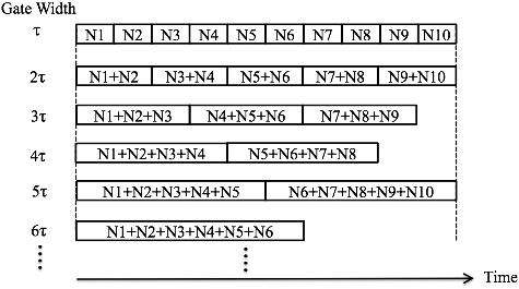
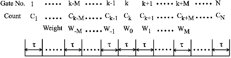
First, the conventional bunching technique is briefly described. Here, it is assumed that time-sequence detection pulses from a pulse-type neutron detector are acquired by an MCS with i_max successive channels, and the ith neutron count stored in the MCS is denoted as N_i (i = 1, 2,…, i_max). The bunching procedure is illustrated in Figure 1, where τ represents a gate width of the MCS and i_max is 10. As seen in this figure, neutron counts within integral multiples of the width τ are synthesized by bunching neutron counts stored in the MCS channels, and the bunch technique has no overlap of adjacent bunches. Consequently, the number of the synthesized data decreases in inverse proportion to the gate width elongated. From the synthesized time-sequence count data, the Y values of the longer gate widths are calculated and the prompt-neutron decay constant can be determined from a least-squares fit of a familiar Feynman-α formula to the Y data. The above feature implies that the statistical scatter may be more significant as the gate width is elongated.

Figure 1. Illustration of the conventional bunching procedure.

2.2. Present moving–bunching technique

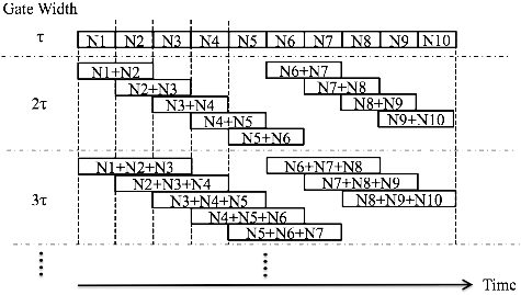
Next, the moving–bunching technique is presented. This bunching procedure is illustrated in Figure 2. As shown in this figure, neutron counts within longer gate widths are synthesized in a similar manner as the conventional technique but the present technique makes adjacent bunches overlap as long as possible. Consequently, the number of the synthesized count data slightly decreases. When i_max is much large, i.e., the registered data length is very long, the decrease of the number of data synthesized is negligible even for much longer gate widths. In this study, time-sequence count data within integral multiples of a gate width of an MCS are synthesized by the present bunching technique and the Y values of the synthesized count data are calculated. The prompt-neutron decay constant is determined from a least-squares fit of the conventional Feynman-α formula to the above Y values. The present bunching technique uses the counts of an MCS channel multiple times to synthesize time-sequence counts within longer time width. Appendix theoretically shows that the multiple uses never influence the Y value and the conventional Feynman-α formula is available in this analysis. The proof is derived from a general Feynman-α formula taking account of filtering processing [5]. The present synthesis procedure is expected to reduce a statistical scatter of the Y data similarly to the moving average technique.

Figure 2. Illustration of the present bunching procedure.

3. Reactor configuration and experimental setups

A Feynman-α experiment was performed in the UTR-KINKI reactor of Kinki University Atomic Energy Research Institute. The UTR-KINKI reactor is a lightwater-moderated, graphite-reflected two-core reactor. The maximum thermal power is only 1 W. The reactor configuration and neutron detector location are shown in Figure 3. The fuel material is contained in two distinct core tanks separated by 18 in. (45.7 cm) of graphite. The graphite region between the tanks has been employed as a standard irradiation field. Additional graphite surrounding the tanks acts as a neutron reflector. The reactor has four control rods in symmetrical positions. In these rods, two are assigned as safety rods for reactor scram and manual shutdown, and are referred to as safety rods #1 and #2, respectively. Others are a shim-safety rod for scram and coarse adjustment of reactivity, and a regulating rod for auto operation and fine adjustment of reactivity. The Feynman-α experiment was carried out at two subcritical states, where the subcritical reactivity was adjusted by changing the axial positions of the above rods. These experimental rod patterns are shown in Table 1, where the reference reactivity is also included. The subcritical reactivity was predetermined by the rod drop method. The above subcritical system was driven by a startup neutron source.

Figure 3. Reactor configuration and detector location.

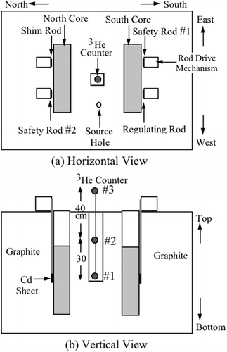
Table 1. Control rod patterns employed in the present experiment.

	Rod position				Reactivity
Pattern	Safety #1	Safety #2	Shim	Regulating	[%Δk/k]
A	U.L.	U.L.	L.L.	U.L.	−0.368
D	L.L.	L.L.	L.L.	L.L.	−1.672

Note: L.L. – lower limit, U.L. – upper limit.

The time-sequence count data were acquired from three ³He proportional counters (0.5 in. diameter), which were placed at different axial positions in an irradiation cavity. As shown in Figure 3, counter #1 was close to the core, while counter #3 was placed far from the core. The nuclear instrumentation system consisted of detector bias supply, preamplifier, spectroscopy amplifier, and discriminator modules. Finally, pulse signals from these neutron counters were fed to a time-sequence data acquisition system, which registered the arriving time of the signal as digital data. The time length of the acquired data was about 10 min. Time-sequence count data within a time interval of 1 ms were generated from the arriving time data and then the count data within longer intervals were synthesized by both the conventional bunching technique and the present moving–bunching one to calculate the Y data.

4. Results and discussion

First, we discuss the applicability of the above two bunching techniques to a neutron counter #3 placed far from the core. Considering the counter location, we expect that the Y must be statistically scattered. Figure 4 shows the gate-width dependence of the Y, where the control rod pattern is A. As expected above, the conventional bunching technique results in a significantly scattered Y, from which the prompt-neutron decay constant is never determinable. However, the present technique surprisingly leads to a typical gate-width dependence of Y in Feynman-α analysis. The advantage of the present technique for such an ex-core detector can be confirmed. 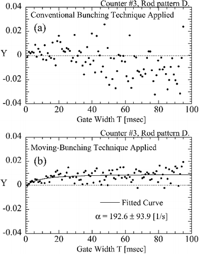The decay constant α could be determined from fitting the following equation to the Y data: (1) $$Y\left(T\right)=Y_{\infty }\left[1-\left(1-e^{-\alpha T}\right)/\alpha T\right],$$(1) where T represented the gate width elongated by the bunching. The above saturated correlation amplitude Y_∞ includes detection efficiency for total fission events, Diven factor [6], reactivity, and effective delayed-neutron fraction. In this figure, a fitted curve of the above equation and the decay constant obtained from the fitting are also indicated. As the error of the decay constant, the standard deviation originated from the least-squares fit is employed. Figure 5 shows the gate-width dependence of the Y, where the control rod pattern is D. At the deeply subcritical state, the conventional bunching technique results in a more significantly scattered Y and most of the Y has negative values in the long gate-width range. The least-squares fit to these scattered data is impossible. On the other hand, the present bunching technique remarkably reduces the scatter and the decay constant is barely determinable from the fitting to the Y data. As indicated in this figure, however, the obtained decay constant has a larger error.

Figure 4. Applicability of different bunching techniques to time-sequence data detected by a neutron counter far from the core at rod pattern A: (a) conventional bunching technique applied; (b) moving–bunching technique applied.

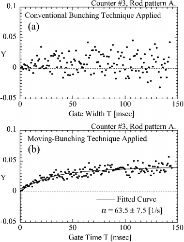
Figure 5. Applicability of different bunching techniques to time-sequence data detected by a neutron counter far from core at rod pattern D: (a) conventional bunching technique applied; (b) moving–bunching technique applied.

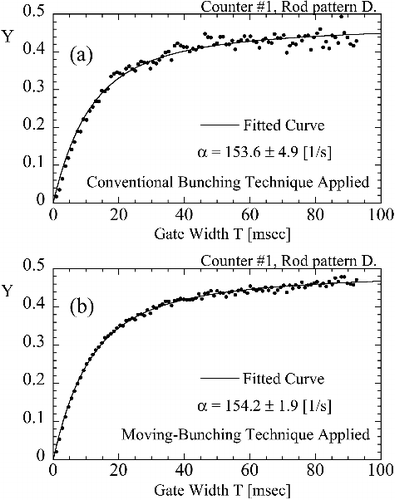
Next, we discuss the applicability of the two bunching techniques to a neutron counter #1 placed closely to the core. Figure 6 shows the gate-width dependence of the Y, where control rod pattern is D. Both the conventional technique and the present one result in a typical gate-width distribution of the Feynman-α analysis. The application of the present technique evidently reduces a scatter of the Y in the long gate-width range and a statistical error of the decay constant. As mentioned above, the present bunching technique is remarkably advantageous for an ex-core detector far from the core. The application of the present technique to another detector close to the core gives an improvement of statistical error.

Figure 6. Applicability of different bunching techniques to time-sequence data detected by a neutron counter close to core at rod pattern D: (a) conventional bunching technique applied; (b) moving–bunching technique applied.

The prompt-neutron decay constants obtained by this study are summarized in Table 2, where “Failed” indicates that the nonlinear least-squares fit to the scattered Y data never produce meaningful results. In a control rod pattern A, i.e., at a slightly subcritical state, the present bunching technique gives the consistent decay constant among three neutron counters. In another control rod pattern D, i.e., at a deeply subcritical state, the present technique also gives the consistent decay constant and reduces the statistical error of the constant.

Table 2. Prompt-neutron decay constant obtained by Feynman-α analysis [1/s].

	Conventional bunching technique			Present bunching technique
Rod Pattern	Counter #1	Counter #2	Counter #3	Counter #1	Counter #2	Counter #3
A	67.1 ± 0.7	71.4 ± 1.1	Failed	66.6 ± 0.2	64.8 ± 0.4	63.5 ± 7.5
D	153.6 ± 4.9	144.6 ± 8.1	Failed	154.2 ± 1.9	151.1 ± 3.0	192.6 ± 93.9

5. Conclusion

An alternative technique referred to as “moving–bunching technique” was proposed to reduce a statistical scatter of variance-to-mean ratio of neutron counts. A Feynman-α experiment was performed in the UTR-KINKI, to confirm the advantage of the proposed bunching technique. When a neutron detector was placed far from the core, a Feynman-α analysis with the conventional bunching technique led to a scattered variance-to-mean ratio from which the prompt-neutron decay constant was never determinable. However, the present analysis with the proposed moving–bunching technique gave a successful result even for such an ex-core detector. For a neutron detector close to the core, the proposed technique resulted in a certain reduction of statistical error of the decay constant.

Disclosure statement

No potential conflict of interest was reported by the authors.

Appendix.  Proof of applicability of the conventional Feynman-α formula

The present moving–bunching technique uses the counts of an MCS channel multiple times to synthesize time-sequence counts within longer time width. This appendix theoretically shows that the multiple uses never influence the Y value and the conventional Feynman-α formula is available in this analysis. First, we briefly describe a filtering technique developed for the Feynman-α analysis.

Consider a correlation analysis of time-sequence data as shown in Figure A1. The counts of a detector within consecutive gates are continuously registered, where gates are opened during a certain time interval (gate width) τ. To these data, Hashimoto et al. [5] applied the following discrete filter: (A1) $$B_k=\sum _{i=-M}^M{w}_i{C}_{k+i},$$(A1) where C_{k + i} and w_i represented the counts within (k + i)th gate and the weight for the counts, respectively, and where B_k indicated the value filtered over the count data of (2M + 1) gates. Here they introduced the following modified variance-to-mean ratio of the counts: (A2) $$\sigma \left(\tau \right)=\frac{1}{N-2M}\sum _{k=1+M}^{N-M}\frac{{(B_k-\bar{B})}^2}{\bar{C}},$$(A2) where N is the total number of gates corresponding to a time length of time-sequence data, and $\bar{C}$ and $\bar{B}$ are the expected values defined as follows: (A3) $$\bar{C}=\frac{1}{N}\sum _{k=1}^N{C}_k,\bar{B}=\frac{1}{N-2M}\sum _{k=1+M}^{N-M}{B}_k.$$(A3)

Figure A1. Filtering over (2M + 1) gates.

According to Equations (21)–(23) of their paper, the modified ratio defined by Equation (A2)(A2) $$\sigma \left(\tau \right)=\frac{1}{N-2M}\sum _{k=1+M}^{N-M}\frac{{(B_k-\bar{B})}^2}{\bar{C}},$$(A2) could be formulated as (A4) $$\sigma \left(\tau \right)=\theta \left\{1+2ϵD_{\nu }\sum _{p=1}^7\frac{A_{p}T\left(s_p\right)}{s_p}{f}_p\left(\tau \right)\right\},$$(A4) (A5) $$\theta =\sum _{i=-M}^M{w}_i^2,$$(A5) (A6) $$f_p\left(\tau \right)=1-\sum _{i=-M}^M\sum _{j=-M}^M{w}_i{w}_j\left\{exp(-\left|i-j\right|\tau s_p)-exp(-\left|i-j+1\right|\tau s_p)\right\}/\phantom{\left\{exp(-\left|i-j\right|\tau s_p)-exp(-\left|i-j+1\right|\tau s_p)\right\}\left(\theta \tau s_p\right)}\left(\theta \tau s_p\right),$$(A6) where D_ν and ϵ represents the Diven factor and detector efficiency, respectively. The above parameters s_p are poles of the zero-power transfer function T(s), and the coefficients A_p are residues corresponding to the poles. The derivation of the above equations is based on the zero-power one-point kinetics model and six-group model for delayed neutron.

Here, we neglect delayed-neutron contribution to reduce Equations (A4)(A4) $$\sigma \left(\tau \right)=\theta \left\{1+2ϵD_{\nu }\sum _{p=1}^7\frac{A_{p}T\left(s_p\right)}{s_p}{f}_p\left(\tau \right)\right\},$$(A4) and (A6(A6) $$f_p\left(\tau \right)=1-\sum _{i=-M}^M\sum _{j=-M}^M{w}_i{w}_j\left\{exp(-\left|i-j\right|\tau s_p)-exp(-\left|i-j+1\right|\tau s_p)\right\}/\phantom{\left\{exp(-\left|i-j\right|\tau s_p)-exp(-\left|i-j+1\right|\tau s_p)\right\}\left(\theta \tau s_p\right)}\left(\theta \tau s_p\right),$$(A6) ) to (A7) $$\sigma \left(\tau \right)=\theta \left\{1+2ϵD_{\nu }\frac{AT\left(\alpha \right)}{\alpha }f\left(\tau \right)\right\},$$(A7) (A8) $$f\left(\tau \right)=1-\sum _{i=-M}^M\sum _{j=-M}^M{w}_i{w}_j\left\{exp(-\left|i-j\right|\tau \alpha )-exp(-\left|i-j+1\right|\tau \alpha )\right\}/\phantom{\left\{exp(-\left|i-j\right|\tau \alpha )-exp(-\left|i-j+1\right|\tau \alpha )\right\}\left(\theta \tau \alpha \right)}\left(\theta \tau \alpha \right),$$(A8) where the parameter α is a maximum pole, i.e., prompt-neutron decay constant, and A is a residue corresponding to α.

On the other hand, the present moving–bunching technique can be described as (A9) $$B_k=\sum _{i=-M}^M{C}_{k+i},$$(A9) (A10) $$Y\left(T\right)=\frac{1}{N-2M}\sum _{k=1+M}^{N-M}\frac{{(B_k-\bar{B})}^2}{\bar{B}}-1=\frac{\bar{C}}{\bar{B}}\sigma \left(\tau \right)-1,$$(A10) (A11) $$T=(2M+1)\tau .$$(A11)

Compare Equation (A1)(A1) $$B_k=\sum _{i=-M}^M{w}_i{C}_{k+i},$$(A1) with Equation (A9)(A9) $$B_k=\sum _{i=-M}^M{C}_{k+i},$$(A9) . When the weight for counts is set as (A12) $$\begin{array}{ccc}\hfill w_{-M}& =& w_{-M+1}=\cdots =w_0=\cdots \hfill \\ & =& w_{M-1}=w_M=1,\hfill \end{array}$$(A12) the general formula for discrete filtering can be reduced to that for the present bunching technique. Substituting Equation (A12)(A12) $$\begin{array}{ccc}\hfill w_{-M}& =& w_{-M+1}=\cdots =w_0=\cdots \hfill \\ & =& w_{M-1}=w_M=1,\hfill \end{array}$$(A12) in Equations (A5)(A5) $$\theta =\sum _{i=-M}^M{w}_i^2,$$(A5) and (A8(A8) $$f\left(\tau \right)=1-\sum _{i=-M}^M\sum _{j=-M}^M{w}_i{w}_j\left\{exp(-\left|i-j\right|\tau \alpha )-exp(-\left|i-j+1\right|\tau \alpha )\right\}/\phantom{\left\{exp(-\left|i-j\right|\tau \alpha )-exp(-\left|i-j+1\right|\tau \alpha )\right\}\left(\theta \tau \alpha \right)}\left(\theta \tau \alpha \right),$$(A8) ), we obtain (A13) $$\theta =2M+1,$$(A13) (A14) $$f\left(\tau \right)=1-\frac{1-exp\left\{-(2M+1)\tau \alpha \right\}}{(2M+1)\tau \alpha }.$$(A14)

The above equations are substituted in Equa-tion (A7)(A7) $$\sigma \left(\tau \right)=\theta \left\{1+2ϵD_{\nu }\frac{AT\left(\alpha \right)}{\alpha }f\left(\tau \right)\right\},$$(A7) to obtain (A15) $$\begin{array}{ccc}\hfill \sigma \left(\tau \right)& =& (2M+1)+2ϵD_{\nu }\frac{AT\left(\alpha \right)}{\alpha }(2M+1)\hfill \\ & & \times \left[1-\frac{1-exp\left\{-(2M+1)\tau \alpha \right\}}{(2M+1)\tau \alpha }\right].\hfill \end{array}$$(A15)

Substituting Equation (A9)(A9) $$B_k=\sum _{i=-M}^M{C}_{k+i},$$(A9) in Equation (A3)(A3) $$\bar{C}=\frac{1}{N}\sum _{k=1}^N{C}_k,\bar{B}=\frac{1}{N-2M}\sum _{k=1+M}^{N-M}{B}_k.$$(A3) , we obtain (A16) $$\bar{B}=\frac{1}{N-2M}\sum _{k=1+M}^{N-M}\sum _{i=-M}^M{C}_{k+i}=(2M+1)\bar{C}.$$(A16)

Substituting Equations (A15(A15) $$\begin{array}{ccc}\hfill \sigma \left(\tau \right)& =& (2M+1)+2ϵD_{\nu }\frac{AT\left(\alpha \right)}{\alpha }(2M+1)\hfill \\ & & \times \left[1-\frac{1-exp\left\{-(2M+1)\tau \alpha \right\}}{(2M+1)\tau \alpha }\right].\hfill \end{array}$$(A15) ) and (A16(A16) $$\bar{B}=\frac{1}{N-2M}\sum _{k=1+M}^{N-M}\sum _{i=-M}^M{C}_{k+i}=(2M+1)\bar{C}.$$(A16) ) in Equa-tion (A10)(A10) $$Y\left(T\right)=\frac{1}{N-2M}\sum _{k=1+M}^{N-M}\frac{{(B_k-\bar{B})}^2}{\bar{B}}-1=\frac{\bar{C}}{\bar{B}}\sigma \left(\tau \right)-1,$$(A10) , we obtain the following conventional formula for the Feynman-α method:(A17) $$Y\left(T\right)=Y_{\infty }\left[1-\frac{1-exp\left(-\alpha T\right)}{\alpha T}\right],$$(A17) where (A18) $$Y_{\infty }=2ϵD_{\nu }\frac{AT\left(\alpha \right)}{\alpha }.$$(A18)

As shown in Equation (A11)(A11) $$T=(2M+1)\tau .$$(A11) , the gate width T elongated by the bunching is confined to an odd multiple of τ. However, the above equation also holds for an even multiple of τ. When the weight for counts is set as (A19) $$\begin{array}{ccc}\hfill w_{-M}& =& w_{-M+1}=\cdots =w_0=\cdots \hfill \\ & =& w_{M-1}=1,\mathrm{and}{w}_M=0,\hfill \end{array}$$(A19) the identical equation to Equation (A17)(A17) $$Y\left(T\right)=Y_{\infty }\left[1-\frac{1-exp\left(-\alpha T\right)}{\alpha T}\right],$$(A17) for an even multiple of τ can be derived. Therefore, it can be concluded that the multiple uses of the counts of an MCS channel never influence the Y value and the conventional Feynman-α formula is available in the present analysis.

References

- Feynman R P, Hoffmann F, Serber R. Dispersion of the neutron emission in U-235 fission. J Nucl Sci Energy. 1956;3:64–69.
- Misawa T, Shiroya S, Kanda K. Measurement of prompt-neutron decay constant and large subcriticality by the Feynman-alpha method. Nucl Sci Eng. 1990;104:53–65.
- Wakabayashi G, Yonemura Y, Heguri H, et al. Measurement of subcritical reactivity in unsteady state with digital time-series data acquisition system using difference filter technique. IEEE Trans Nucl Sci. 2002;49:2508–2512.
- Tonoike K, Yamamoto T, Watanabe S, et al. Real time α value measurement with Feynman-α method utilizing time series data acquisition on low enriched uranium system. J Nucl Sci Technol. 2004;41:177–182.
- Hashimoto K, Ohsaki H, Horiguchi T, et al. Variance-to-mean method generalized by linear filter technique. Ann Nucl Energy. 1998;25:639–652.
- Diven DC, Martin HC, Taschek RF, et al. Multiplicities of fission neutrons. Phys Rev. 1956;101:1012–1015.