Bias factor method using random sampling technique

ABSTRACT

Toward the practical use of the bias factor method for actual light water reactor core analyses, the bias factor method using the random sampling technique is newly proposed. The bias factor method is one of the correction methods using information of E/C values in existing measurable systems, to reduce biases and uncertainties of predicted core characteristics parameters. By the aid of the random sampling technique, our proposed bias factor method can be carried out using only forward calculations without any adjoint calculations, and can easily take into account burnup and thermal-hydraulic feedback effects, which are difficult points in the practical application to actual core analyses. Although the statistical error due to the random sampling technique is inevitable in the proposed method, the statistical error can be simply quantified by the resampling technique such as the bootstrap method. As one of the feasibility studies, effectiveness of the proposed method is verified through a numerical experiment which virtually simulates a typical equilibrium pressurized water reactor core. In this verification problem, it is clarified that E/C values of control rod worth at the beginning of cycle under the hot zero power condition are useful information to reduce biases and uncertainties of predicted assembly-wise power distributions during operation of hot full power.

Keywords:

• Bias factor method
• random sampling
• bootstrap method
• bias
• uncertainty
• covariance
• correlation
• numerical analysis

1. Introduction

In the core design for an advanced reactor and the design of fuel loading pattern in an existing reactor, safety of nuclear reactor is ensured in advance by the core analysis, where core characteristics parameters (CCP) (e.g. excess reactivity, control rod worth (CRW), reactivity coefficients, and peaking factor) are numerically predicted. Thus, accuracy and precision of predicted CCPs are important to ensure the safety of designed reactor. Improvement of evaluated nuclear data (e.g. JENDL-4.0 [1,2] and ENDF/B-VII.1 [3]), numerical analysis methods (e.g. MOC assembly calculation [4] followed by the pin-by-pin core analysis [5]), and computer performance contributes to more accurate and precise prediction. Nevertheless, numerical results of core analysis have biases and uncertainties due to various factors: one of the factors is the analytical modeling error (e.g. discretizing error in the deterministic code and statistical error and insufficient modeling in the Monte Carlo code) and another factor is the uncertainty of input parameters (e.g. fabrication tolerance of density, nuclide composition, and size; and uncertainty of nuclear data). Among of these factors, the uncertainty of nuclear data (i.e. the covariance data of evaluated nuclear data library) could be a major factor.

In order to reduce biases and uncertainties of predicted CCPs in the light water reactor (LWR) core analysis, the authors proposed the cross-section adjustment technique on the basis of the random sampling (RS) technique [6,7]. Generally, a complicated two-step calculation scheme (e.g. lattice physics calculation followed by core calculation) is adapted in the recent LWR core analysis; thus, the treatment of burnup and thermal-hydraulic feedback effects is one of the challenging issues in the practical application of the cross-section adjustment technique to the actual LWR core analysis. The use of the RS technique enables us to easily take into account the burnup and thermal-hydraulic feedback effects, compared with an adjoint-based approach [8,9]. In the case of cross-section adjustment technique, the input parameters of nuclear data are updated to reproduce measured CCPs in existing measurable systems (e.g. criticality experimental facility, mockup core, and existing commercial reactor). As another approach to reduce biases and uncertainties of predicted CCPs, the bias factor method has also been investigated by many researchers [10–13]. In the case of bias factor method, the outputs of predicted CCPs in designed cores are corrected using the information of E/C values (i.e. the ratio of experimental results to calculation results) in existing measurable systems. Here, the E/C value is called as the “bias factor,” which represents the correction factor in the bias factor method. In comparison with the cross-section adjustment technique, the bias factor method is a correction technique for outputs and does not require further recalculation of core analysis. However, the applicability of RS technique to the bias factor method is not fully investigated so far.

In the present paper, we aim to propose the bias factor method using the RS technique. Features of our proposed method are briefly described as follows:

1.	Any adjoint calculations are not necessary. Existing core analysis code system can be used without major modification.
2.	Burnup and thermal-hydraulic feedback effects can be easily taken into account.
3.	Any number and kind of CCPs ${\overrightarrow{R}}^{\left(1\right)}$ can be used for the information of E/C values in existing measurable systems.
4.	Any number and kind of CCPs ${\overrightarrow{R}}^{\left(2\right)}$ in the designed cores can be corrected. Note that it requires strong correlations between ${\overrightarrow{R}}^{\left(2\right)}$ and ${\overrightarrow{R}}^{\left(1\right)}$ to effectively reduce uncertainties of corrected ${\overrightarrow{R}}^{\left(2\right)}$, as discussed in Section 3.
5.	Total calculation time depends only on the total number of random sampling and does not depend on the number of input parameters and CCPs for correction. Here, the statistical error can be estimated by the resampling technique such as the bootstrap method [14–16].

The contents of the present paper are as follows: In Section 2, methodology of the bias factor method using the RS technique is explained. Section 3 shows verification through a virtual equilibrium core analysis for a typical four-loop pressurized water reactor (PWR). Finally, concluding remarks are summarized in Section 4.

2. Methodology

First of all, in order to derive the bias factor method using the RS technique, it is assumed that CCPs ${\overrightarrow{R}}_{\exp }^{\left(1\right)}={\left\{r_{\exp ,1}^{\left(1\right)},r_{\exp ,2}^{\left(1\right)},...,r_{\exp ,n_1}^{\left(1\right)}\right\}}^T$ are obtained in measurable systems, where ${\overrightarrow{R}}_{\exp }^{\left(1\right)}$ is a n₁-dimensional column vector which consists of various kinds of CCPs, i.e. total number of experimental results is n₁. By numerical analysis for these experiments with an evaluated nuclear data, we can obtain the corresponding numerical results, denoted as ${\overrightarrow{R}}_{\mathrm{calc}}^{\left(1\right)}$. In addition, CCPs ${\overrightarrow{R}}_{\mathrm{calc}}^{\left(2\right)}={\left\{r_{\mathrm{calc},1}^{\left(2\right)},r_{\mathrm{calc},2}^{\left(2\right)},...,r_{\mathrm{calc},n_2}^{\left(2\right)}\right\}}^T$ in designed cores can be also calculated with the same nuclear data, where n₂ means the total number of calculation results in the design cores.

Now, let us assume that a priori probabilities of ${\overrightarrow{R}}_{\exp }^{\left(1\right)}$ and ${\overrightarrow{R}}^{\left(2\right)}$ are expressed by multivariate normal distributions $\mathcal{N}\left({\overrightarrow{R}}_{\exp }^{\left(1\right)}\right|{\overrightarrow{R}}_{\mathrm{calc}}^{\left(1\right)},{\Sigma }_{11})$ and $\mathcal{N}\left({\overrightarrow{R}}^{\left(2\right)}\right|{\overrightarrow{R}}_{\mathrm{calc}}^{\left(2\right)},{\Sigma }_{22})$, respectively, where $\mathcal{N}\left(\overrightarrow{x}\right|\overrightarrow{\mu },\Sigma )$ means a normal distribution with mean $\overrightarrow{\mu }$ and covariance matrix Σ for a random variable vector $\overrightarrow{x}$, and Σ_ii is a covariance matrix among ${\overrightarrow{R}}^{\left(i\right)}$. Then, a conditional probability (or a posteriori probability) $p\left({\overrightarrow{R}}^{\left(2\right)}\right|{\overrightarrow{R}}_{\exp }^{\left(1\right)})$ can be derived as a multivariate normal distribution $\mathcal{N}\left({\overrightarrow{R}}^{\left(2\right)}\right|{\overrightarrow{R}}_{2|1}^{\left(2\right)},{\Sigma }_{2|1})$, where a posteriori mean ${\overrightarrow{R}}_{2|1}^{\left(2\right)}$ and covariance Σ_2|1 are evaluated as follows [17]: (1) $${\overrightarrow{R}}_{2|1}^{\left(2\right)}={\overrightarrow{R}}_{\mathrm{calc}}^{\left(2\right)}+{\Sigma }_{21}{\Sigma }_{11}^{-1}\left({\overrightarrow{R}}_{\exp }^{\left(1\right)}-{\overrightarrow{R}}_{\mathrm{calc}}^{\left(1\right)}\right),$$(1) (2) $${\Sigma }_{2|1}={\Sigma }_{22}-{\Sigma }_{21}{\Sigma }_{11}^{-1}{\Sigma }_{12},$$(2) where Σ₁₂ indicates covariance matrix between ${\overrightarrow{R}}_{\exp }^{\left(1\right)}$ and ${\overrightarrow{R}}^{\left(2\right)}$; Σ₂₁ is the transposed matrix of Σ₁₂, i.e. Σ₂₁ = Σ^T₁₂ ; and Σ^{− 1}₁₁ means the inverse matrix of Σ₁₁. To further transform Equations (1)(1) $${\overrightarrow{R}}_{2|1}^{\left(2\right)}={\overrightarrow{R}}_{\mathrm{calc}}^{\left(2\right)}+{\Sigma }_{21}{\Sigma }_{11}^{-1}\left({\overrightarrow{R}}_{\exp }^{\left(1\right)}-{\overrightarrow{R}}_{\mathrm{calc}}^{\left(1\right)}\right),$$(1) and (2(2) $${\Sigma }_{2|1}={\Sigma }_{22}-{\Sigma }_{21}{\Sigma }_{11}^{-1}{\Sigma }_{12},$$(2) ), following uncertainties are assumed:

1.	Uncertainties of calculated results for ${\overrightarrow{R}}^{\left(1\right)}$ and ${\overrightarrow{R}}^{\left(2\right)}$ due to the covariance of evaluated nuclear data: V(11)XS, V(22)XS, and V(12)XS.
2.	Experimental errors for ${\overrightarrow{R}}_{\exp }^{\left(1\right)}$: V(11)exp.
3.	Analytical modeling errors for ${\overrightarrow{R}}^{\left(1\right)}$ and ${\overrightarrow{R}}^{\left(2\right)}$: V(11)model, V(22)model, and V(12)model.

Here, V^(ij) indicates covariance matrix between ${\overrightarrow{R}}^{\left(i\right)}$ and ${\overrightarrow{R}}^{\left(j\right)}$; and it is assumed that there are no correlations among uncertainties due to nuclear data, experimental errors, and analytical modeling errors. Then, covariance matrices Σ₁₁, Σ₂₂, and Σ₁₂ can be decomposed into the following expressions: (3) $${\Sigma }_{11}={\mathbf{V}}_{\mathrm{XS}}^{\left(11\right)}\mathit{}+{\mathbf{V}}_{\exp }^{\left(11\right)}+{\mathbf{V}}_{\mathrm{model}}^{\left(11\right)},$$(3) (4) $${\Sigma }_{22}={\mathbf{V}}_{\mathrm{XS}}^{\left(22\right)}\mathit{}+{\mathbf{V}}_{\mathrm{model}}^{\left(22\right)},$$(4) (5) $${\Sigma }_{12}={\mathbf{V}}_{\mathrm{XS}}^{\left(12\right)}\mathit{}+{\mathbf{V}}_{\mathrm{model}}^{\left(12\right)}$$(5)

By using the RS technique based on the covariance of nuclear data, V^(ij)_XS is estimated as follows: (6) $$\begin{array}{ccc}\hfill {\mathbf{V}}_{\mathrm{XS}}^{\left(ij\right)}& \approx & \mathrm{cov}\left({\overrightarrow{R}}_{\mathrm{calc}}^{\left(i\right)},{\overrightarrow{R}}_{\mathrm{calc}}^{\left(j\right)}\right)\equiv \frac{1}{N-1}\hfill \\ & & \times \sum _{k=1}^N\left({\overrightarrow{R}}_{\mathrm{calc},k}^{\left(i\right)}-{\overrightarrow{R}}_{\mathrm{ave}}^{\left(i\right)}\right){\left({\overrightarrow{R}}_{\mathrm{calc},k}^{\left(j\right)}-{\overrightarrow{R}}_{\mathrm{ave}}^{\left(j\right)}\right)}^T,\hfill \end{array}$$(6) (7) $${\overrightarrow{R}}_{\mathrm{ave}}^{\left(i\right)}=\frac{1}{N}\sum _{k=1}^N{\overrightarrow{R}}_{\mathrm{calc},k}^{\left(i\right)},$$(7) where ${\overrightarrow{R}}_{\mathrm{calc},k}^{\left(i\right)}$ is a vector of CCPs for kth sampled nuclear data, and N is the total number of random samples. Finally, by substituting Equations (3)(3) $${\Sigma }_{11}={\mathbf{V}}_{\mathrm{XS}}^{\left(11\right)}\mathit{}+{\mathbf{V}}_{\exp }^{\left(11\right)}+{\mathbf{V}}_{\mathrm{model}}^{\left(11\right)},$$(3) , (4(4) $${\Sigma }_{22}={\mathbf{V}}_{\mathrm{XS}}^{\left(22\right)}\mathit{}+{\mathbf{V}}_{\mathrm{model}}^{\left(22\right)},$$(4) ), and (5(5) $${\Sigma }_{12}={\mathbf{V}}_{\mathrm{XS}}^{\left(12\right)}\mathit{}+{\mathbf{V}}_{\mathrm{model}}^{\left(12\right)}$$(5) ) into Equations (1)(1) $${\overrightarrow{R}}_{2|1}^{\left(2\right)}={\overrightarrow{R}}_{\mathrm{calc}}^{\left(2\right)}+{\Sigma }_{21}{\Sigma }_{11}^{-1}\left({\overrightarrow{R}}_{\exp }^{\left(1\right)}-{\overrightarrow{R}}_{\mathrm{calc}}^{\left(1\right)}\right),$$(1) and (2(2) $${\Sigma }_{2|1}={\Sigma }_{22}-{\Sigma }_{21}{\Sigma }_{11}^{-1}{\Sigma }_{12},$$(2) ), theoretical formula for the bias factor method using the RS technique can be derived as follows: (8) $${\overrightarrow{R}}_{2|1}^{\left(2\right)}={\overrightarrow{R}}_{\mathrm{calc}}^{\left(2\right)}+\mathbf{K}\left({\overrightarrow{R}}_{\exp }^{\left(1\right)}-{\overrightarrow{R}}_{\mathrm{calc}}^{\left(1\right)}\right),$$(8) (9) $$\begin{array}{ccc}\hfill {\Sigma }_{2|1}& =& \mathrm{cov}\left({\overrightarrow{R}}_{\mathrm{calc}}^{\left(2\right)},{\overrightarrow{R}}_{\mathrm{calc}}^{\left(2\right)}\right)+{\mathbf{V}}_{\mathrm{model}}^{\left(22\right)}\hfill \\ & & -\mathbf{K}\left(\mathrm{cov}\left({\overrightarrow{R}}_{\mathrm{calc}}^{\left(1\right)},{\overrightarrow{R}}_{\mathrm{calc}}^{\left(2\right)}\right)+{\mathbf{V}}_{\mathrm{model}}^{\left(12\right)}\right),\hfill \end{array}$$(9) (10) $$\begin{array}{ccc}& & \mathbf{K}\equiv \left(\mathrm{cov}\left({\overrightarrow{R}}_{\mathrm{calc}}^{\left(2\right)},{\overrightarrow{R}}_{\mathrm{calc}}^{\left(1\right)}\right)+{\mathbf{V}}_{\mathrm{model}}^{\left(21\right)}\right)\hfill \\ & & \times {\left(\mathrm{cov}\left({\overrightarrow{R}}_{\mathrm{calc}}^{\left(1\right)},{\overrightarrow{R}}_{\mathrm{calc}}^{\left(1\right)}\right)+{\mathbf{V}}_{\exp }^{\left(11\right)}+{\mathbf{V}}_{\mathrm{model}}^{\left(11\right)}\right)}^{-1}.\hfill \end{array}$$(10)

Equations (8)(8) $${\overrightarrow{R}}_{2|1}^{\left(2\right)}={\overrightarrow{R}}_{\mathrm{calc}}^{\left(2\right)}+\mathbf{K}\left({\overrightarrow{R}}_{\exp }^{\left(1\right)}-{\overrightarrow{R}}_{\mathrm{calc}}^{\left(1\right)}\right),$$(8) –(10(10) $$\begin{array}{ccc}& & \mathbf{K}\equiv \left(\mathrm{cov}\left({\overrightarrow{R}}_{\mathrm{calc}}^{\left(2\right)},{\overrightarrow{R}}_{\mathrm{calc}}^{\left(1\right)}\right)+{\mathbf{V}}_{\mathrm{model}}^{\left(21\right)}\right)\hfill \\ & & \times {\left(\mathrm{cov}\left({\overrightarrow{R}}_{\mathrm{calc}}^{\left(1\right)},{\overrightarrow{R}}_{\mathrm{calc}}^{\left(1\right)}\right)+{\mathbf{V}}_{\exp }^{\left(11\right)}+{\mathbf{V}}_{\mathrm{model}}^{\left(11\right)}\right)}^{-1}.\hfill \end{array}$$(10) ) are identical to the formulae which are utilized in the derivation process for the extended cross-section adjustment method [18]. Namely, our proposed bias factor method provides essentially the same results of ${\overrightarrow{R}}_{2|1}^{\left(2\right)}$ as the extended cross-section adjustment method. Using Equations (8)(8) $${\overrightarrow{R}}_{2|1}^{\left(2\right)}={\overrightarrow{R}}_{\mathrm{calc}}^{\left(2\right)}+\mathbf{K}\left({\overrightarrow{R}}_{\exp }^{\left(1\right)}-{\overrightarrow{R}}_{\mathrm{calc}}^{\left(1\right)}\right),$$(8) –(10(10) $$\begin{array}{ccc}& & \mathbf{K}\equiv \left(\mathrm{cov}\left({\overrightarrow{R}}_{\mathrm{calc}}^{\left(2\right)},{\overrightarrow{R}}_{\mathrm{calc}}^{\left(1\right)}\right)+{\mathbf{V}}_{\mathrm{model}}^{\left(21\right)}\right)\hfill \\ & & \times {\left(\mathrm{cov}\left({\overrightarrow{R}}_{\mathrm{calc}}^{\left(1\right)},{\overrightarrow{R}}_{\mathrm{calc}}^{\left(1\right)}\right)+{\mathbf{V}}_{\exp }^{\left(11\right)}+{\mathbf{V}}_{\mathrm{model}}^{\left(11\right)}\right)}^{-1}.\hfill \end{array}$$(10) ), a priori predicted values of ${\overrightarrow{R}}_{\mathrm{calc}}^{\left(2\right)}$ can be updated to the corrected values of ${\overrightarrow{R}}_{2|1}^{\left(2\right)}$ with the reduced covariance matrices of Σ_2|1.

In order to clarify the relationship with E/C values of ${\overrightarrow{R}}^{\left(1\right)}$ (denoted as ${\overrightarrow{f}}^{\left(1\right)}$), let us transform Equation (8)(8) $${\overrightarrow{R}}_{2|1}^{\left(2\right)}={\overrightarrow{R}}_{\mathrm{calc}}^{\left(2\right)}+\mathbf{K}\left({\overrightarrow{R}}_{\exp }^{\left(1\right)}-{\overrightarrow{R}}_{\mathrm{calc}}^{\left(1\right)}\right),$$(8) into Equation (11)(11) $${\overrightarrow{f}}_{2|1}={\overrightarrow{1}}_{n_2}+{\mathbf{K}}^{\text{'}}\left({\overrightarrow{f}}^{\left(1\right)}-{\overrightarrow{1}}_{n_1}\right),$$(11) : (11) $${\overrightarrow{f}}_{2|1}={\overrightarrow{1}}_{n_2}+{\mathbf{K}}^{\text{'}}\left({\overrightarrow{f}}^{\left(1\right)}-{\overrightarrow{1}}_{n_1}\right),$$(11) (12) $${\overrightarrow{f}}_{2|1}\equiv \mathrm{dia}{\mathrm{g}}^{-1}\left({\overrightarrow{R}}_{\mathrm{calc}}^{\left(2\right)}\right){\overrightarrow{R}}_{2|1}^{\left(2\right)},$$(12) (13) $$\begin{array}{ccc}\hfill {\overrightarrow{f}}^{\left(1\right)}& \equiv & \mathrm{dia}{\mathrm{g}}^{-1}\left({\overrightarrow{R}}_{\mathrm{calc}}^{\left(1\right)}\right){\overrightarrow{R}}_{\exp }^{\left(1\right)}\hfill \\ & =& {\left\{r_{\exp ,1}^{\left(1\right)}/r_{\mathrm{calc},1}^{\left(1\right)},...,r_{\exp ,n_1}^{\left(1\right)}/r_{\mathrm{calc},n_1}^{\left(1\right)}\right\}}^T,\hfill \end{array}$$(13) (14) $${\mathbf{K}}^{\text{'}}\equiv \mathrm{dia}{\mathrm{g}}^{-1}\left({\overrightarrow{R}}_{\mathrm{calc}}^{\left(2\right)}\right)\mathbf{K}\mathit{}\mathrm{diag}\left({\overrightarrow{R}}_{\mathrm{calc}}^{\left(1\right)}\right),$$(14) (15) $$\mathrm{diag}\left(\overrightarrow{x}\right)\equiv \left[\begin{array}{ccc}\hfill x_1& \hfill \cdots & \hfill 0\\ \hfill ⋮& \hfill \ddots & \hfill ⋮\\ \hfill 0& \hfill \cdots & \hfill x_n\end{array}\right],$$(15) (16) $$\mathrm{dia}{\mathrm{g}}^{-1}\left(\overrightarrow{x}\right)\equiv \left[\begin{array}{ccc}\hfill 1/x_1& \hfill \cdots & \hfill 0\\ \hfill ⋮& \hfill \ddots & \hfill ⋮\\ \hfill 0& \hfill \cdots & \hfill 1/x_n\end{array}\right],$$(16) where $\overrightarrow{x}={\left\{x_1,x_2,...,x_n\right\}}^T$, and ${\overrightarrow{1}}_n$ is the n-dimensional column vector where all elements are unity, i.e. ${\overrightarrow{1}}_n={\left\{1,1,...,1\right\}}^T$. In Equation (13)(13) $$\begin{array}{ccc}\hfill {\overrightarrow{f}}^{\left(1\right)}& \equiv & \mathrm{dia}{\mathrm{g}}^{-1}\left({\overrightarrow{R}}_{\mathrm{calc}}^{\left(1\right)}\right){\overrightarrow{R}}_{\exp }^{\left(1\right)}\hfill \\ & =& {\left\{r_{\exp ,1}^{\left(1\right)}/r_{\mathrm{calc},1}^{\left(1\right)},...,r_{\exp ,n_1}^{\left(1\right)}/r_{\mathrm{calc},n_1}^{\left(1\right)}\right\}}^T,\hfill \end{array}$$(13) , each element of ${\overrightarrow{f}}^{\left(1\right)}$ represents the “individual bias factor” for ${\overrightarrow{R}}_{\mathrm{calc}}^{\left(1\right)}$ [11,12]. In addition, ${\overrightarrow{f}}_{2|1}$ means a vector of bias factors for ${\overrightarrow{R}}_{\mathrm{calc}}^{\left(2\right)}$, i.e. ${\overrightarrow{R}}_{\mathrm{calc}}^{\left(2\right)}$ is modified to ${\overrightarrow{R}}_{2|1}^{\left(2\right)}$ by multiplying the diagonal matrix $\mathrm{diag}\left({\overrightarrow{f}}_{2|1}\right)$. As shown in Equation (11)(11) $${\overrightarrow{f}}_{2|1}={\overrightarrow{1}}_{n_2}+{\mathbf{K}}^{\text{'}}\left({\overrightarrow{f}}^{\left(1\right)}-{\overrightarrow{1}}_{n_1}\right),$$(11) , the bias factors ${\overrightarrow{f}}_{2|1}$ can be acquired using the individual bias factors ${\overrightarrow{f}}^{\left(1\right)}$ with the matrix K′ which is related to the correlation between ${\overrightarrow{R}}^{\left(1\right)}$ and ${\overrightarrow{R}}^{\left(2\right)}$.

The RS technique is based on the sampling technique, thus the statistical error is inevitable. However, analytical estimation of the statistical error is difficult, since the calculation procedures of ${\overrightarrow{R}}_{2|1}^{\left(2\right)}$ and Σ_2|1 are complicated as shown in Equations (8)(8) $${\overrightarrow{R}}_{2|1}^{\left(2\right)}={\overrightarrow{R}}_{\mathrm{calc}}^{\left(2\right)}+\mathbf{K}\left({\overrightarrow{R}}_{\exp }^{\left(1\right)}-{\overrightarrow{R}}_{\mathrm{calc}}^{\left(1\right)}\right),$$(8) --(10(10) $$\begin{array}{ccc}& & \mathbf{K}\equiv \left(\mathrm{cov}\left({\overrightarrow{R}}_{\mathrm{calc}}^{\left(2\right)},{\overrightarrow{R}}_{\mathrm{calc}}^{\left(1\right)}\right)+{\mathbf{V}}_{\mathrm{model}}^{\left(21\right)}\right)\hfill \\ & & \times {\left(\mathrm{cov}\left({\overrightarrow{R}}_{\mathrm{calc}}^{\left(1\right)},{\overrightarrow{R}}_{\mathrm{calc}}^{\left(1\right)}\right)+{\mathbf{V}}_{\exp }^{\left(11\right)}+{\mathbf{V}}_{\mathrm{model}}^{\left(11\right)}\right)}^{-1}.\hfill \end{array}$$(10) ). In order to easily estimate the statistical errors of ${\overrightarrow{R}}_{2|1}^{\left(2\right)}$ and Σ_2|1, the bootstrap method can be utilized [14–16]. In the case of the uncertainty quantification using the RS technique, the estimation procedure and the verification of statistical error using the bootstrap method were previously reported by the authors [16]. Detailed procedures in the bias factor method are described below:

1.	An original dataset of CCPs $X=\left\{\left({\overrightarrow{R}}_{\mathrm{calc},1}^{\left(1\right)},{\overrightarrow{R}}_{\mathrm{calc},1}^{\left(2\right)}\right),...,\left({\overrightarrow{R}}_{\mathrm{calc},N}^{\left(1\right)},{\overrightarrow{R}}_{\mathrm{calc},N}^{\left(2\right)}\right)\right\}$ is provided by the RS technique. Here, a pair $\left({\overrightarrow{R}}_{\mathrm{calc},k}^{\left(1\right)},{\overrightarrow{R}}_{\mathrm{calc},k}^{\left(2\right)}\right)$ is calculated on the basis of kth sampled nuclear data (1 ⩽ k ⩽ N).
2.	By “random sampling with replacement” from the original dataset X, a resample (so-called “bootstrap sample”) is newly generated as $X^{*}=\left\{\left({\overrightarrow{R}}_{\mathrm{calc},1}^{\left(1\right)*},{\overrightarrow{R}}_{\mathrm{calc},1}^{\left(2\right)*}\right),...,\left({\overrightarrow{R}}_{\mathrm{calc},N}^{\left(1\right)*},{\overrightarrow{R}}_{\mathrm{calc},N}^{\left(2\right)*}\right)\right\}$, where the superscript * represents the bootstrap sample. Here, it is noted that “random sampling with replacement” is one of the technical terms in statistics, i.e. each element in the original data has an equal probability to be selected and it is permissible to be redundantly selected. Namely, each element $\left({\overrightarrow{R}}_{\mathrm{calc},r}^{\left(1\right)*},{\overrightarrow{R}}_{\mathrm{calc},r}^{\left(2\right)*}\right)$ is randomly selected from all elements of X, using an uniform random number within the range of [1, N]. In other words, r is determined as r =  ξ, where ξ means a uniform random integer number (1 ⩽ ξ ⩽ N).
3.	The bootstrap samples X*b are repeatedly resampled (b = 1, 2, …, B), where B is the total number of bootstrap samples.
4.	For each bootstrap sample X*b, the “bootstrap replicates” of ${\overrightarrow{R}}_{2|1}^{\left(2\right)*b}$ and Σ*b2|1 are evaluated as follows: (17) $${\overrightarrow{R}}_{2|1}^{\left(2\right)*b}={\overrightarrow{R}}_{\mathrm{calc}}^{\left(2\right)}+{\mathbf{K}}^{*b}\left({\overrightarrow{R}}_{\exp }^{\left(1\right)}-{\overrightarrow{R}}_{\mathrm{calc}}^{\left(1\right)}\right),$$(17) (18) $$\begin{array}{ccc}\hfill {\Sigma }_{2|1}^{*b}& =& \mathrm{cov}\left({\overrightarrow{R}}_{\mathrm{calc}}^{\left(2\right)*b},{\overrightarrow{R}}_{\mathrm{calc}}^{\left(2\right)*b}\right)+{\mathbf{V}}_{\mathrm{model}}^{\left(22\right)}\hfill \\ & & -{\mathbf{K}}^{*b}\left(\mathrm{cov}\left({\overrightarrow{R}}_{\mathrm{calc}}^{\left(1\right)*b},{\overrightarrow{R}}_{\mathrm{calc}}^{\left(2\right)*b}\right)+{\mathbf{V}}_{\mathrm{model}}^{\left(12\right)}\right),\hfill \end{array}$$(18) (19) $$\begin{array}{ccc}& & {\mathbf{K}}^{*b}\equiv \left(\mathrm{cov}\left({\overrightarrow{R}}_{\mathrm{calc}}^{\left(2\right)*b},{\overrightarrow{R}}_{\mathrm{calc}}^{\left(1\right)*b}\right)+{\mathbf{V}}_{\mathrm{model}}^{\left(21\right)}\right)\hfill \\ & & \times {\left(\mathrm{cov}\left({\overrightarrow{R}}_{\mathrm{calc}}^{\left(1\right)*b},{\overrightarrow{R}}_{\mathrm{calc}}^{\left(1\right)*b}\right)+{\mathbf{V}}_{\exp }^{\left(11\right)}+{\mathbf{V}}_{\mathrm{model}}^{\left(11\right)}\right)}^{-1}.\hfill \end{array}$$(19) Consequently, B bootstrap replicates ${\overrightarrow{R}}_{2|1}^{\left(2\right)*1},...,{\overrightarrow{R}}_{2|1}^{\left(2\right)*B}$ and Σ*12|1, …, Σ2|1*B are obtained to estimate statistical errors of ${\overrightarrow{R}}_{2|1}^{\left(2\right)}$ and Σ2|1.
5.	In the case of percentile method, the confidence intervals of ${\overrightarrow{R}}_{2|1}^{\left(2\right)}$ and Σ2|1 are simply estimated by percentile points for the B bootstrap replicates ${\overrightarrow{R}}_{2|1}^{\left(2\right)*b}$ and Σ*b2|1. Or, statistical errors (1σ) of ${\overrightarrow{R}}_{2|1}^{\left(2\right)}$ and Σ2|1 are estimated as standard deviations for ${\overrightarrow{R}}_{2|1}^{\left(2\right)*b}$ and Σ*b2|1.

3. Verification

3.1. Calculation condition

In the present study, our proposed bias factor method is verified by a virtual numerical experiment, which simulates a typical operation of PWR core under a realistic condition considering thermal hydraulics feedback and cycle burnup effects. In this numerical experiment, virtual true values of CCPs of ${\overrightarrow{R}}^{\left(1\right)}$ and ${\overrightarrow{R}}^{\left(2\right)}$ are artificially produced using a core analysis code with a certain set of input parameters such as perturbed nuclear data. Then, virtual measurement values of ${\overrightarrow{R}}_{\exp }^{\left(1\right)}$ are also numerically simulated by adding experimental errors to the virtual true values of ${\overrightarrow{R}}^{\left(1\right)}$. By utilizing these virtual true and measurement values of CCPs, we investigate whether biases and uncertainties of target CCPs ${\overrightarrow{R}}^{\left(2\right)}$can be effectively reduced by the proposed bias factor methods. For this purpose, CASMO4/SIMULATE3 with L-library is used as an example of the licensing grade simulator for LWR core analysis [19,20]. Here, the L-library is a 70 energy group microscopic cross-section library for CASMO4.

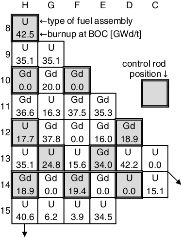
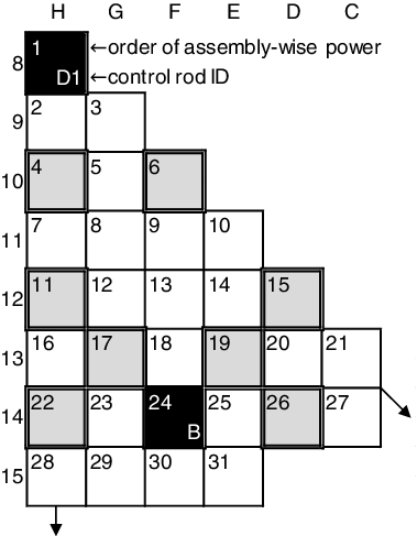
As the target of bias factor method, we focused on a typical four-loop 17 × 17 PWR equilibrium core with the 15.9 GWd/t operating cycle. Figure 1 shows the core loading pattern, which satisfies octant core symmetry although the core analysis itself was carried out by full core calculation. Two types of fuel assemblies were loaded in the core: One consists of 264 fuel rods of 4.8wt%-UO₂, where the ²³⁵U enrichment is 4.8wt% (denoted as U), and another consists of 240 fuel rods of 4.8wt%-UO₂ and 24 fuel rods of 10wt% Gadolinia bearing 3.2wt%-UO₂ (denoted as Gd). In order to obtain the equilibrium core, burnup calculations for nine successive cycles with the same loading pattern were carried out, followed by the burnup calculation for the target cycle 10.

Figure 1. Core loading pattern of equilibrium core.

In order to evaluate $\mathrm{cov}\left({\overrightarrow{R}}_{\mathrm{calc}}^{\left(i\right)},{\overrightarrow{R}}_{\mathrm{calc}}^{\left(j\right)}\right)$ in Equations (8)(8) $${\overrightarrow{R}}_{2|1}^{\left(2\right)}={\overrightarrow{R}}_{\mathrm{calc}}^{\left(2\right)}+\mathbf{K}\left({\overrightarrow{R}}_{\exp }^{\left(1\right)}-{\overrightarrow{R}}_{\mathrm{calc}}^{\left(1\right)}\right),$$(8) –(10(10) $$\begin{array}{ccc}& & \mathbf{K}\equiv \left(\mathrm{cov}\left({\overrightarrow{R}}_{\mathrm{calc}}^{\left(2\right)},{\overrightarrow{R}}_{\mathrm{calc}}^{\left(1\right)}\right)+{\mathbf{V}}_{\mathrm{model}}^{\left(21\right)}\right)\hfill \\ & & \times {\left(\mathrm{cov}\left({\overrightarrow{R}}_{\mathrm{calc}}^{\left(1\right)},{\overrightarrow{R}}_{\mathrm{calc}}^{\left(1\right)}\right)+{\mathbf{V}}_{\exp }^{\left(11\right)}+{\mathbf{V}}_{\mathrm{model}}^{\left(11\right)}\right)}^{-1}.\hfill \end{array}$$(10) ), the RS technique was applied to generate 200 perturbed L-libraries on the basis the covariance data in JENDL-4.0(u) [1,2]. In the present study, we used the covariance data of capture, fission, and elastic scattering (σ_c, σ_f, σ_s), and the number of neutrons emitted per fission ($\bar{\nu }$) only for 18 heavy nuclides (²³⁴U, ²³⁵U, ²³⁶U, ²³⁸U, ²³⁷Np, ²³⁸Pu, ²³⁹Pu, ²⁴⁰Pu, ²⁴¹Pu, ²⁴²Pu, ²⁴¹Am, ²⁴²Am, ²⁴³Am, ²⁴²Cm, ²⁴³Cm, ²⁴⁴Cm, ²⁴⁵Cm, ²⁴⁶Cm), which are considered as major contributors for uncertainties of core characteristics in LWR analyses. Note that cross-section uncertainty of fission products and other nuclides are not taken into account since covariance data for many of these nuclides have not been evaluated. The detailed procedure of the RS technique has been already reported by the authors [7,16]. By a sequence of depletion calculations for cycles 1 (initial core) through 10 (target core) with kth perturbed L-libraries, the corresponding CCPs ${\overrightarrow{R}}_{\mathrm{calc},k}^{\left(i\right)}$ were evaluated. Namely depletion calculations for cycles 1–10 were carried out for 200 times.

We aimed to reduce biases and uncertainties of CCPs at the cycle 10 under the hot full power (HFP) condition. Following CCPs, which correspond to ${\overrightarrow{R}}^{\left(2\right)}$ in Equations (8)(8) $${\overrightarrow{R}}_{2|1}^{\left(2\right)}={\overrightarrow{R}}_{\mathrm{calc}}^{\left(2\right)}+\mathbf{K}\left({\overrightarrow{R}}_{\exp }^{\left(1\right)}-{\overrightarrow{R}}_{\mathrm{calc}}^{\left(1\right)}\right),$$(8) –(10(10) $$\begin{array}{ccc}& & \mathbf{K}\equiv \left(\mathrm{cov}\left({\overrightarrow{R}}_{\mathrm{calc}}^{\left(2\right)},{\overrightarrow{R}}_{\mathrm{calc}}^{\left(1\right)}\right)+{\mathbf{V}}_{\mathrm{model}}^{\left(21\right)}\right)\hfill \\ & & \times {\left(\mathrm{cov}\left({\overrightarrow{R}}_{\mathrm{calc}}^{\left(1\right)},{\overrightarrow{R}}_{\mathrm{calc}}^{\left(1\right)}\right)+{\mathbf{V}}_{\exp }^{\left(11\right)}+{\mathbf{V}}_{\mathrm{model}}^{\left(11\right)}\right)}^{-1}.\hfill \end{array}$$(10) ), were the target of the bias factor method:

1.	HFP critical boron concentration (CBC) from the beginning of cycle (BOC) to the end of cycle (EOC), i.e. 0 through 15.9 GWd/t.
2.	HFP assembly-wise power distribution at the BOC, the middle of cycle (MOC) 7 GWd/t, and the EOC.

In this verification problem, ${\overrightarrow{R}}^{\left(2\right)}$ represents CCPs during HFP operation, which can be predicted by the core burnup calculation using CASMO4/SIMULATE3. In the present numerical experiment, numerical results ${\overrightarrow{R}}_{\mathrm{calc},T}^{\left(2\right)}$ obtained by another randomly sampled L-library (denoted as Tth perturbed L-libraries) were regarded as the virtual true values of ${\overrightarrow{R}}^{\left(2\right)}$.

As measureable CCPs ${\overrightarrow{R}}^{\left(1\right)}$ for the bias factor method, we assumed the following two cases of CCPs at the BOC of cycle 10 under the hot zero power (HZP) condition:

Case 1: Only HZP CBC.

Case 2: HZP CBC and HZP CRW at 10 positions in core as shown in Figure 1.

Namely, in this problem, ${\overrightarrow{R}}^{\left(1\right)}$ corresponds to CCPs, which can be measured by zero power reactor physics experiments in an actual PWR. By the aid of E/C values of ${\overrightarrow{R}}^{\left(1\right)}$, predicted values of ${\overrightarrow{R}}^{\left(2\right)}$ during operation were updated by the bias factor method. Here, measurement values of ${\overrightarrow{R}}_{\exp }^{\left(1\right)}$ were virtually generated by adding experimental errors to the virtual true values ${\overrightarrow{R}}_{\mathrm{calc},T}^{\left(1\right)}$. Here, it was assumed that the experimental errors of ${\overrightarrow{R}}^{\left(1\right)}$ follow normal distributions with standard deviations of 0.1 ppm and 0.1 pcm for HZP CBC and HZP CRW, respectively. Note that there were no correlations among experimental errors of HZP CBC and HZP CRW. Namely, V⁽¹¹⁾_exp is a diagonal matrix and all of non-diagonal elements, which correspond to covariance between different measurement values, are zero. Furthermore, in this verification problem, experimental values were virtually obtained by the same core analysis code, thus analytical modeling errors V⁽¹¹⁾_model, V⁽²²⁾_model, and V⁽¹²⁾_model were assumed to be zero.

3.2. Results and discussion

In this section, results of reduced biases and uncertainties by the bias factor method are shown and discussed. Here, the bias is defined as the difference between predicted and true values, i.e. ${\overrightarrow{R}}_{\mathrm{calc}}^{\left(2\right)}-{\overrightarrow{R}}_{\mathrm{calc},T}^{\left(2\right)}$ or ${\overrightarrow{R}}_{2|1}^{\left(2\right)}-{\overrightarrow{R}}_{\mathrm{calc},T}^{\left(2\right)}$; and the uncertainty is defined as the square root of diagonal element of Σ₂₂ or Σ_2|1, i.e. standard deviation (1σ).

Table 1 shows results of HFP CBC. In the case of no correction, bias is the largest at the BOC, and becomes to be smaller as the cycle burnup increases. In Case 1, biases and uncertainties near the BOC can be reduced, since the measurement values of HZP CBC were used in the bias factor method. However, the bias in Case 1 tends to be large with increase of the cycle burnup, although the bias falls within the range of uncertainty. On the other hand, Case 2 utilizes additional information of E/C values of HZP CRW, which strongly correlate to the assembly-wise power distribution. As discussed in the latter parts of this section, Case 2 can improve the precision and accuracy of the HFP assembly-wise power distribution. The power distribution has significant impact on the burnup distribution, which is dominant factor for the criticality, or the CBC. Thus, biases and uncertainties in Case 2 can be further improved over the whole cycle burnup.

Table 1. Biases and uncertainties (σ) of HFP CBC (ppm).

Burnup	No correction		Case 1		Case 2
[GWd/t]	Bias	σ	Bias	σ	Bias	σ
0.0	20.5	69.0	0.1	0.4	−0.2	0.3
0.1	19.5	68.3	−0.7	1.4	−0.5	0.6
0.5	18.9	68.4	−1.3	1.5	−0.7	0.6
1.0	18.3	68.6	−1.9	2.5	−0.8	0.7
3.0	15.9	69.7	−4.6	7.4	−1.4	1.3
5.0	13.4	70.8	−7.2	11.7	−2.2	1.9
7.0	11.4	71.6	−9.3	15.2	−3.0	2.4
9.0	9.7	72.3	−10.9	18.1	−3.6	3.0
11.0	7.9	72.8	−12.7	20.7	−4.7	3.7
13.0	6.4	73.2	−14.1	23.0	−5.6	4.7
15.0	5.0	73.5	−15.4	25.3	−6.5	5.6
15.9	4.6	73.6	−15.7	26.3	−6.7	5.9

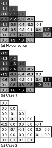
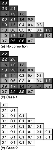
Next, as an example of HFP assembly-wise power distributions, biases and uncertainties at the BOC are shown in Figures 2 and 3, respectively. As a summary, Table 2 shows root-mean-square and maximum values of the biases and uncertainties. As shown in Table 2, regardless of with or without the bias factor method, biases and uncertainties of the HFP assembly-wise power tends to be smaller as the cycle burnup increases; thus let us focus on results at the BOC to discuss the effectiveness of the bias factor method. In the case of no correction, it is interesting to note that the biases and uncertainties of the HFP assembly-wise power tend to be small in an intermediate region between the center and the periphery of core. The perturbations due to uncertainty of nuclear data results in excitation of spatial higher modes of neutron flux. The present core loading pattern has octant symmetry, thereby the excitation of higher modes related to the azimuthal angle direction could be drastically suppressed. Namely, higher order modes related to the radial direction are more likely to be excited, as discussed in the authors' previous research [21]. Consequently, the symmetrical loading pattern of PWR results in “in-out” power tilt due to the covariance data of nuclear data. That is why the biases and uncertainties of HFP assembly-wise power distributions are small at the core intermediate region, which corresponds to nodal points (zero points) of the higher mode related to the radial direction. Although the bias factor method of Case 1 enables to improve the accuracy and precision of the HFP CBC near the BOC, the biases of HFP assembly-wise power of Case 1 get slightly worse and its uncertainties are nearly equal to those in the case of no correction. Namely, the information of E/C value of HZP CBC has a little contribution to the improvement of accuracy and precision of HFP assembly-wise power distribution. On the other hand, both biases and uncertainties of HFP assembly-wise power are dramatically improved over the whole core by Case 2, where additional 10 measurement values of HZP CRW are utilized in the bias factor method.

Figure 2. Bias of HFP assembly-wise power (%) at BOC.

Figure 3. Uncertainty of HFP assembly-wise power (%) at BOC.

Table 2. Biases and uncertainties (σ) of HFP assembly-wise power distribution (%).

	(a) Root-mean-square
	No correction		Case 1		Case 2
	Bias	σ	Bias	σ	Bias	σ
BOC	0.8	1.5	0.9	1.5	0.1	0.1
MOC	0.3	0.7	0.4	0.7	0.1	0.1
EOC	0.1	0.5	0.2	0.5	0.1	0.1
	(b) Maximum of absolute value
	No correction		Case 1		Case 2
	Bias	σ	Bias	σ	Bias	σ
BOC	1.3	2.6	1.6	2.5	0.2	0.1
MOC	0.5	1.3	0.6	1.3	0.2	0.2
EOC	0.3	1.0	0.4	0.9	0.2	0.2

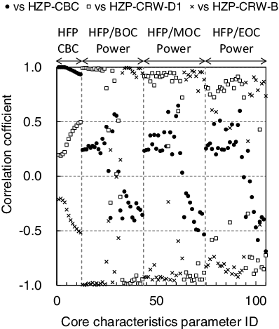
In order to discuss the reason why Case 2 is superior to Case 1, Figure 4 shows correlation coefficients between ${\overrightarrow{R}}^{\left(1\right)}$ (HZP CBC and HZP CRW at the positions D1 and B as shown in Figure 5) and ${\overrightarrow{R}}^{\left(2\right)}$. In Figure 4, “core characteristics parameter ID” (CCP ID) of the x-axis is an index for CCPs of ${\overrightarrow{R}}^{\left(2\right)}$, and defined as follows:

Figure 4. Correlation coefficients between ${\overrightarrow{R}}^{\left(1\right)}$ and ${\overrightarrow{R}}^{\left(2\right)}$.

Figure 5. Sequential order of assembly-wise power for CCP ID.

1-12: HFP CBC from the BOC to the EOC in ascending order.

13-43: HFP assembly-wise power at the BOC from the center to the periphery in sequential order as shown in Figure 5.

44-74: HFP assembly-wise power at the MOC, in the same order as the BOC.

75-105: HFP assembly-wise power at the EOC, in the same order as the BOC and the MOC.

As shown in Figure 4, HZP CBC has strong correlation to HFP CBC (i.e. the correlation coefficient ranges from 1.00 to 0.93) but relatively weak to HFP assembly-wise power distribution (i.e. the correlation coefficient varies within the range of ± 0.6). Thus, Case 1 cannot improve the accuracy and precision of HFP assembly-wise power distribution. On the other hand, HZP CRW values at D1 and B have strong correlation to the inner and the outer assembly-wise powers, respectively. Combination of various measured CCPs such as Case 2 mutually compensates the strongly correlated CCPs of ${\overrightarrow{R}}^{\left(2\right)}$ to cover the entire range of the CCP ID. Consequently, Case 2 can more effectively reduce the biases and uncertainties than Case 1. As discussed earlier, strongly correlated CCPs between experimental and calculation values are useful information to accurately predict CCPs in non-measurable system with small uncertainties. This knowledge is consistent to the authors' previous investigation about the uncertainty reduction method for CCPs of which measurement values are not obtained [22]. Although the present verification problem is one of the feasibility studies which simulate a zero power reactor experiment in the actual PWR, the present study implies that the zero power reactor experiment is very useful to reduce biases and uncertainties of predicted CCPs during operation.

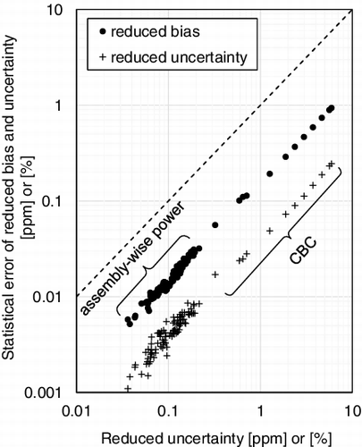
Last, Figure 6 shows bootstrap statistical errors of the bias factor method using the RS technique for Case 2. In Figure 6, x-axis indicates the reduced uncertainty of ${\overrightarrow{R}}^{\left(2\right)}$ (i.e. the square root of diagonal element of Σ_2|1) for each of CCPs, and y-axis indicates the corresponding statistical errors of reduced biases and uncertainties. As shown in Figure 6, in the case of N = 200, the bootstrap statistical errors of reduced biases and uncertainties are approximately 1/6 and 1/25 of the reduced uncertainties, respectively. In this way, the statistical error of the RS technique can be quantified using the bootstrap method, which is useful information to determine the total number of random samples N in our proposed bias factor method.

Figure 6. Bootstrap statistical errors of reduced biases and uncertainties for Case 2.

4. Conclusion

In the present paper, the bias factor method using the RS technique was proposed to avoid troublesome adjoint calculations and to easily treat the burnup and thermal-hydraulic feedback effects in the actual LWR core analysis. Although the statistical error inevitably occurs in the case of the RS technique, the statistical error can be quantified using the resampling technique such as the bootstrap method. Through the numerical experiment which virtually simulates a typical PWR core analysis, it is verified that the bias factor method with various measured CCPs can further improve the accuracy and precision of predicted CCPs in the designed core (or the non-measurable system). In addition, it is reconfirmed that CCPs, which have strong correlations between experimental and calculation values, make an important role in the bias factor method. In the case of present verification problem, HZP CRW at the BOC strongly correlates to HFP assembly-wise power during operation, depending on the position of control rod. Thus, E/C values of HZP CRW at the BOC are useful information to reduce biases and uncertainties of the predicted HFP assembly power distribution.

For the practical application of our proposed method to an actual LWR core, one of the future tasks is to establish how to evaluate the experimental errors V⁽¹¹⁾_exp and the analytical modeling errors V^(ij)_model. Furthermore, in order to evaluate more reliable uncertainty V^(ij)_XS due to evaluated nuclear data, it is also necessary to properly take into account covariance data of the fission product and the fission yield.

Acknowledgements

We sincerely appreciate Nuclear Fuel Industries, Ltd., for the technical supports for the use of randomly sampled microscopic cross-section libraries.

Disclosure statement

No potential conflict of interest was reported by the authors.

Additional information

Funding

This work was supported in part by JSPS KAKENHI, Grant-in-Aid for Scientific Research (C) [Grant Number 24561040].

References

- Shibata K, Iwamoto O, Nakagawa T, et al. JENDL-4.0: a new library for nuclear science and engineering. J Nucl Sci Technol. 2011;48:1–30.
- JENDL-4.0u [Internet]. Japan: Japan Atomic Energy Agency; 2012 Sep 14 [updated 2015 Sep 14; cited 2015 Sep 22]. Available from: http://wwwndc.jaea.go.jp/jendl/j40/update/
- Chadwick MB, Herman M, Obložinský P, et al. ENDF/B-VII.1 nuclear data for science and technology: cross sections, covariances, fission product yields and decay data. Nucl Data Sheets. 2011;112:2887–2996.
- Yamamoto A, Endo T, Tabuchi M, et al. AEGIS: an advanced lattice physics code for light water reactor analyses. Nucl Eng Technol. 2010;42:500–519.
- Tatsumi M, Yamamoto A. Advanced PWR core calculation based on multi-group nodal-transport method in three-dimensional pin-by-pin geometry. J Nucl Sci Technol. 2003;40:376–387.
- Kato S, Endo T, Yamamoto A, et al. Random sampling-based cross-section adjustment technique for LWR core analysis. Paper presented at: 2013 International Congress on Advances in Nuclear Power Plants (ICAPP'13); 2013 Apr 14–18; Jeju Island, Korea.
- Watanabe T, Endo T, Yamamoto A, et al. Cross section adjustment method based on random sampling technique. J Nucl Sci Technol. 2014;51:590–599.
- Hara A, Takeda T, Kikuchi Y. SAGEP: two-dimensional sensitivity analysis code based on generalized perturbation theory. Ibaraki (Japan): Japan Atomic Energy Agency; 1984 ( JAERI-M 84-027).
- Chiba G, Tsuji M, Narabayashi T. Uncertainty quantification of neutronic parameters of light water reactor fuel cells with JENDL-4.0 covariance data. J Nucl Sci Technol. 2013;50:751–760.
- Kamei T, Yoshida T. Error due to nuclear data uncertainties in the prediction of large liquid-metal fast breeder reactor core performance parameters. Nucl Sci Eng. 1983;84:83–97.
- Sano T, Takeda T. Generalized bias factor method for accurate prediction of neutronic characteristics. J Nucl Sci Technol. 2006;43:1465–1470.
- Kugo T, Mori T, Takeda T. Theoretical study on new bias factor methods to effectively use critical experiments for improvement of prediction accuracy of neutronic characteristics. J Nucl Sci Technol. 2007;44:1509–1517.
- Kugo T, Andoh M, Kojima K, et al. Prediction accuracy improvement of neutronics characteristics of a breeding light water reactor core by extended bias factor methods with use of FCA-XXII-1 critical experiments. J Nucl Sci Technol. 2008;45:288–303.
- Efron B. Bootstrap methods: another look at the Jackknife. Ann Stat. 1979;7:1–26.
- Efron B, Tibshirani RJ. An introduction to the bootstrap. New York (NY): Chapman & Hall; 1993.
- Endo T, Watanabe T, Yamamoto A. Confidence interval estimation by bootstrap method for uncertainty quantification using random sampling method. J Nucl Sci Technol. 2015;52:993–999.
- Muirhead RJ. Aspects of multivariate statistical theory. New York (NY): John Wiley & Sons; 1982.
- Yokoyama K, Ishikawa M, Kugo T. Extended cross-section adjustment method to improve the prediction accuracy of core parameters. J Nucl Sci Technol. 2012;49:1165–1174.
- CASMO-4 A Fuel Assembly Burn-up Program. User's manual. Waltham (MA): Studsvik Scandpower Inc; 2009 (SSP-09/443-U Rev 0).
- SIMULATE-3 advanced three-dimensional two-group reactor analysis code. Waltham (MA): Studsvik Scandpower Inc; 2009 (SSP-09/447-U Rev 0).
- Endo T, Ohori K, Yamamoto A. Application of the robust design concept for fuel loading pattern. J Nucl Sci Technol. 2011;48:1077–1086.
- Yamamoto A, Yasue Y, Endo T, et al. Uncertainty estimation of core safety parameters using cross-correlations of covariance matrix. J Nucl Sci Technol. 2013;50:966–978.