Theoretical comparison of performance using transfer functions for reactivity meters based on inverse kinetic method and simple feedback method

ABSTRACT

The performance of two digital reactivity meters, one based on the conventional inverse kinetic method and the other one based on simple feedback theory, are compared analytically using their respective transfer functions. The latter one is proposed by one of the authors. It has been shown that the performance of the two reactivity meters become almost identical when proper system parameters are selected for each reactivity meter. A new correlation between the system parameters of the two reactivity meters is found. With this correlation, filter designers can easily determine the system parameters for the respective reactivity meters to obtain identical performance.

KEYWORDS:

• Reactivity
• nuclear criticality safety
• sub-criticality
• reactivity estimation
• inverse point kinetic equation
• noise filtering

1. Introduction

A new method of estimating the reactivity of a neutron multiplying system has been proposed [1]. It is based on a simple feedback method (referred as Simplest Reactivity Estimator, and hereafter SRE) but has a performance similar to that of the conventional reactivity meter based on inverse kinetic method (referred as inverse point kinetic (IPK) hereafter). The basic theory and qualitative comparison of the performance of both reactivity meters are discussed in the aforementioned paper to show feasibility of SRE reactivity meter. It has also shown that SRE has possibility of better performance than that of IPK for reactivity estimation under noisy environment because of its robust filter characteristics. However, in order to utilize such a new method in actual reactor systems, it must be reviewed and verified carefully by many experts.

Performance of reactivity meters is discussed on good noise filtering and quick response. They are important in certain cases, e.g. for reactivity estimation during low power reactor physics tests, or when monitoring the reactivity in sub-critical systems [2–6]. It is well known that noise-filtering capability sacrifices quick response of calculated reactivity as discussed in the other paper [5]. The noise-filtering capability or time response is dependent on respective system parameter in the reactivity meters, such as the time constant, τ, for the first-order delay digital filter in IPK and the feedback gain adjuster, F, in SRE. The operation experience of the former has accumulated in the long time interval up to today. However, SRE has no such experience. Also the above-mentioned gain adjuster, F, has been empirically introduced in the aforementioned paper for noise filtering. Therefore, no qualitative and theoretical investigations on F have been done. From these points of view, the main objective of this paper is to discuss and clarify the characteristics of the system parameter of gain adjuster, F, in SRE in order to answer the question such as ‘Is it possible and enough to select a proper value for F to guarantee equivalent performance of a SRE reactivity meter with the well experienced conventional IPK reactivity meters?’

For this investigation, theoretical transfer functions are used to compare the performance of the two reactivity meters. Based on the comparison, clarification of the characteristics of F would be helpful for those interested in reactivity meter design. And, if possible, it would be also helpful to give an idea of the relationship of τ and F, as there is no guidance for selecting a proper value for F. Detailed discussions are given how to understand the results and frequency response of the respective transfer functions. Finally, it is shown that SRE could be accepted to use in the actual reactor systems as IPK.

2. Brief explanation of the two types of reactivity meters

In this section, basic introductions are given from reference [1] for convenience.

The point kinetic equation is expressed as follows for a sub-critical system with external neutron source Q: (1) $$\frac{\mathrm{d}n\left(t\right)}{\mathrm{d}t}=\frac{\rho \left(t\right)-\beta }{\ell }n\left(t\right)+\sum _{i=1}^m{\lambda }_i{C}_i\left(t\right)+Q$$(1) (2) $$\frac{\mathrm{d}{C}_i\left(t\right)}{\mathrm{d}t}=\frac{{\beta }_i}{\ell }n\left(t\right)-{\lambda }_i{C}_i\left(t\right)i=1,2,...,m$$(2) (3) $$\beta =\sum _i^m{\beta }_i,$$(3) where ρ(t) denotes the reactivity, n(t) denotes the neutron density, C_i(t) are the precursor decay constants, ℓ denotes the prompt neutron generation time, and Q denotes an independent neutron source. The effective strength of the neutron source has been assumed as constant and expressed [2] in terms of the initial stable sub-criticality as (4) $$Q=\frac{-{\rho }_0{n}_0}{\ell }$$(4) where n₀ denotes the neutron density at an arbitrary, sub-critical steady state and ρ₀ denotes the corresponding reactivity obtained from some other means (such as a reactor physics calculation, or a measurement, e.g. rod drop experiment).

2.1. Inverse point kinetic (IPK) based method

The well-known IPK reactivity is estimated as follows. From the point kinetics models (1(1) $$\frac{\mathrm{d}n\left(t\right)}{\mathrm{d}t}=\frac{\rho \left(t\right)-\beta }{\ell }n\left(t\right)+\sum _{i=1}^m{\lambda }_i{C}_i\left(t\right)+Q$$(1) ) and (2(2) $$\frac{\mathrm{d}{C}_i\left(t\right)}{\mathrm{d}t}=\frac{{\beta }_i}{\ell }n\left(t\right)-{\lambda }_i{C}_i\left(t\right)i=1,2,...,m$$(2) ), the following equation can be derived: (5) $$\rho \left(t\right)=\frac{\ell }{n\left(t\right)}\left[\frac{\mathrm{d}n\left(t\right)}{\mathrm{d}t}+\sum _{i=1}^m\frac{\mathrm{d}{C}_i\left(t\right)}{\mathrm{d}t}-Q\right].$$(5)

Suppose the samples of the neutron density (measurement) are denoted as n_k, obtained at time instant, t = kT_s, k = 0,1,2,…, where T_s is the sampling interval. Then from Equation (2)(2) $$\frac{\mathrm{d}{C}_i\left(t\right)}{\mathrm{d}t}=\frac{{\beta }_i}{\ell }n\left(t\right)-{\lambda }_i{C}_i\left(t\right)i=1,2,...,m$$(2) (6) $$C_{i,k}=e^{-{\lambda }_i{T}_s}{C}_{i,k-1}+\frac{1}{{}_i}\left(1-e^{-{\lambda }_i{T}_s}\right)\frac{{\beta }_i}{\ell }{\widehat{n}}_k,$$(6) where ${\widehat{n}}_k$ is the measured neutron density.

Further, in Equation (5)(5) $$\rho \left(t\right)=\frac{\ell }{n\left(t\right)}\left[\frac{\mathrm{d}n\left(t\right)}{\mathrm{d}t}+\sum _{i=1}^m\frac{\mathrm{d}{C}_i\left(t\right)}{\mathrm{d}t}-Q\right].$$(5) , the derivative can be approximated as (7) $$\frac{\mathrm{d}n}{\mathrm{d}t}{|}_k=\frac{n_k-n_{k-1}}{T_s}$$(7) (8) $$\frac{\mathrm{d}{C}_i}{\mathrm{d}t}{|}_k=\frac{C_{i,k}-C_{i,k-1}}{T_s}$$(8)

And thus,(9) $${\rho }_k=\frac{\ell }{n_k}\left[\frac{n_k-n_{k-1}}{T_s}+\sum _{i=1}^m\frac{C_{i,k}-C_{i,k-1}}{T_s}-Q\right]$$(9) which, along with Equation (6)(6) $$C_{i,k}=e^{-{\lambda }_i{T}_s}{C}_{i,k-1}+\frac{1}{{}_i}\left(1-e^{-{\lambda }_i{T}_s}\right)\frac{{\beta }_i}{\ell }{\widehat{n}}_k,$$(6) , is suitable for implementation on a digital computer. The result will be an approximation of the reactivity at different time instants. If there are strong fluctuations in the neutron density, for instance during a measurement at deep sub-criticality, the reactivity estimates obtained by such a method show significant fluctuations. This is because the IPK equations involve differentiation of the neutron density with respect to time. In fact, Equations (7)(7) $$\frac{\mathrm{d}n}{\mathrm{d}t}{|}_k=\frac{n_k-n_{k-1}}{T_s}$$(7) and (8(8) $$\frac{\mathrm{d}{C}_i}{\mathrm{d}t}{|}_k=\frac{C_{i,k}-C_{i,k-1}}{T_s}$$(8) ) give a derivative over the very small time interval, T_S, and as such this approximation is subject to very quick fluctuations especially neutron density with random noise. To reduce such spurious fluctuations, one needs to apply a filter. First, the differentiation term of the neutron flux can be omitted due to the fact that the magnitude of this term is negligible in comparison with the other terms as adopted in prompt jump approximation; this simplification is widely adopted in digital reactivity meters in actual use [7]. Second, the usual method of smoothing the neutron density fluctuation is to apply a low-pass filter to the measured neutron density before using IPK. The low-pass filter is a digital first-order delay filter which is given as follows:(10) $$n_k=n_{k-1}+\frac{T_s}{T_s+\tau }\left({\widehat{n}}_k-n_{k-1}\right),$$(10) where n_k and n_{k − 1} are filtered neutron density and τ is the time constant of the digital first-order delay filter. Since the time constant of the first-order delay is selected as small as 0.2 sec, accuracy is not lost [7].

2.2. Simple feedback method (SRE)

Application of our new method is limited to sub-critical systems, or slightly super-critical systems such as those expected during reactor physics tests. Under such circumstances, the derivative of the neutron flux is small. Multiplying both sides of Equation (1)(1) $$\frac{\mathrm{d}n\left(t\right)}{\mathrm{d}t}=\frac{\rho \left(t\right)-\beta }{\ell }n\left(t\right)+\sum _{i=1}^m{\lambda }_i{C}_i\left(t\right)+Q$$(1) by the prompt neutron generation time, the following equation is obtained:(11) $$\ell \frac{\mathrm{d}n\left(t\right)}{\mathrm{d}t}=\left(\rho \left(t\right)-\beta \right)n\left(t\right)+\ell \left(\sum _{i=1}^m{\lambda }_i{C}_i\left(t\right)+Q\right).$$(11)

Considering that the product of neutron generation time, ℓ, and dn/dt is small, the left side of Equation (11)(11) $$\ell \frac{\mathrm{d}n\left(t\right)}{\mathrm{d}t}=\left(\rho \left(t\right)-\beta \right)n\left(t\right)+\ell \left(\sum _{i=1}^m{\lambda }_i{C}_i\left(t\right)+Q\right).$$(11) can be set to be zero. This is the familiar prompt jump approximation [8]. (12) $$0=\left(\rho \left(t\right)-\beta \right)n\left(t\right)+\ell \left(\sum _{i=1}^m{\lambda }_i{C}_i\left(t\right)+Q\right).$$(12)

Thus, neutron density can be expressed as (13) $$n\left(t\right)=\frac{\ell \left({\sum }_{i=1}^m{\lambda }_i{C}_i\left(t\right)+Q\right)}{\beta -\rho \left(t\right)}.$$(13)

The proposed new procedure estimates reactivity as follows. The following discussion assumes one family of delayed neutron precursors for the simplicity of explanation. (In the actual application, Equation (13)(13) $$n\left(t\right)=\frac{\ell \left({\sum }_{i=1}^m{\lambda }_i{C}_i\left(t\right)+Q\right)}{\beta -\rho \left(t\right)}.$$(13) is used, i.e. taking into account more than one precursor family.) At the moment, we assume no noise on the measurement neutron density.

Based on the above discussion, the expected neutron density is calculated as (14) $$n_{\exp ,k+1}=\frac{\ell \left(\lambda C_{k+1}+Q\right)}{\beta -{\rho }_k}.$$(14)

Note here that the reactivity in Equation (14)(14) $$n_{\exp ,k+1}=\frac{\ell \left(\lambda C_{k+1}+Q\right)}{\beta -{\rho }_k}.$$(14) is the reactivity determined in the previous time step. The precursor concentrations, C_{k + 1} are calculated from Equation (6)(6) $$C_{i,k}=e^{-{\lambda }_i{T}_s}{C}_{i,k-1}+\frac{1}{{}_i}\left(1-e^{-{\lambda }_i{T}_s}\right)\frac{{\beta }_i}{\ell }{\widehat{n}}_k,$$(6) using the measured neutron density. When the reactivity does not change, the expected neutron density, n_{exp, k + 1} must be identical with the measured neutron flux. However, if the reactivity is assumed to change slightly between the previous measurement and the present time by an amount, δρ, the true (measured) neutron density is (15) $$n_{t,k+1}=\frac{\ell \left(\lambda C_{k+1}+Q\right)}{\beta -\left({\rho }_k+\delta \rho \right)}.$$(15)

The difference of neutron density, δn, between the expected value n_{exp, k + 1} and the measured value n_{t,k + 1} is calculated as (16) $$\begin{array}{ccc}\hfill \delta n& =& \ell \left(\lambda C_{k+1}+Q\right)\left\{\frac{1}{\beta -\left({\rho }_k+\delta \rho \right)}-\frac{1}{\beta -{\rho }_k}\right\}\hfill \\ & =& \ell \left(\lambda C_{k+1}+Q\right)\left\{\frac{\delta \rho }{\left(\beta -{\rho }_k\right)\left\{\beta -\left({\rho }_k+\delta \rho \right)\right\}}\right\}\hfill \end{array}$$(16)

Here, Equation (15)(15) $$n_{t,k+1}=\frac{\ell \left(\lambda C_{k+1}+Q\right)}{\beta -\left({\rho }_k+\delta \rho \right)}.$$(15) is used to get (17) $$\delta n=\frac{\delta \rho }{\beta -{\rho }_k}{n}_{t,k+1}.$$(17)

This is a relation between the difference of the expected and the true neutron density, and the reactivity error. Thus, the correction for the reactivity becomes(18) $$\delta \rho =\frac{\beta -{\rho }_k}{n_{t,k+1}}\delta n=K\delta n.$$(18) where K can be said as feedback gain and expressed as (19) $$K=\frac{\beta -{\rho }_k}{n_{t,k+1}}.$$(19)

Finally, the estimated reactivity is corrected at the k + 1th step as follows: (20) $${\rho }_{k+1}={\rho }_k+\delta \rho .$$(20)

3. Analytical modeling

Transfer functions for the two reactivity meter methods are derived theoretically. For simplicity, but not losing theoretical accuracy, the formulation is carried out using a linearized version of the point kinetic model with one family of delayed neutron precursors.

3.1. Inverse point kinetic (IPK) based method

The above-mentioned point kinetic equations are expressed as follows. (21) $$\frac{\mathrm{d}n\left(t\right)}{\mathrm{d}t}=\frac{\rho \left(t\right)-\beta }{\ell }n\left(t\right)+\lambda C\left(t\right)+Q$$(21) (22) $$\frac{\mathrm{d}C\left(t\right)}{\mathrm{d}t}=\frac{\beta }{\ell }n\left(t\right)-\lambda C\left(t\right)$$(22)

For t ⩽ 0, (23) $$\rho =0,n=n_0\left(\mathrm{constant}\right)\mathrm{and}C=C_0=\frac{\beta n_0}{\lambda \ell }$$(23)

These equations are linearized as follows: (24) $$n\left(t\right)=n_0+\delta n\left(t\right)$$(24) (25) $$C\left(t\right)=C_0+\delta C\left(t\right)$$(25)

Substituting them into Equations (21)(21) $$\frac{\mathrm{d}n\left(t\right)}{\mathrm{d}t}=\frac{\rho \left(t\right)-\beta }{\ell }n\left(t\right)+\lambda C\left(t\right)+Q$$(21) and (22(22) $$\frac{\mathrm{d}C\left(t\right)}{\mathrm{d}t}=\frac{\beta }{\ell }n\left(t\right)-\lambda C\left(t\right)$$(22) ), using the relation of Equations (24)(24) $$n\left(t\right)=n_0+\delta n\left(t\right)$$(24) and (25(25) $$C\left(t\right)=C_0+\delta C\left(t\right)$$(25) ), Equation (21)(21) $$\frac{\mathrm{d}n\left(t\right)}{\mathrm{d}t}=\frac{\rho \left(t\right)-\beta }{\ell }n\left(t\right)+\lambda C\left(t\right)+Q$$(21) is written as (26) $$\frac{\mathrm{d}\mathit{\delta }n\left(t\right)}{\mathrm{d}t}=\frac{\mathit{\rho }\left(t\right)-\mathit{\beta }}{\ell }\mathit{\delta }n\left(t\right)+\mathit{\lambda }\mathbf{\delta }C\left(t\right)+\frac{\mathit{\rho }\left(t\right)}{\ell }{n}_0$$(26)

Since δn, ρ are assumed to be small enough, the product can be neglected. Thus, we obtain linearized equation for Equation (21)(21) $$\frac{\mathrm{d}n\left(t\right)}{\mathrm{d}t}=\frac{\rho \left(t\right)-\beta }{\ell }n\left(t\right)+\lambda C\left(t\right)+Q$$(21) as (27) $$\frac{\mathrm{d}\delta n\left(t\right)}{\mathrm{d}t}=-\frac{\beta }{\ell }\delta n\left(t\right)+\lambda \delta C\left(t\right)+\frac{\rho \left(t\right)}{\ell }{n}_0.$$(27)

Equation (22)(22) $$\frac{\mathrm{d}C\left(t\right)}{\mathrm{d}t}=\frac{\beta }{\ell }n\left(t\right)-\lambda C\left(t\right)$$(22) can be easily linearized as (28) $$\frac{\mathrm{d}\mathit{\delta }C\left(t\right)}{\mathrm{d}t}=\frac{\mathit{\beta }}{\ell }\mathit{\delta }n\left(t\right)-\mathit{\lambda }\mathbf{\delta }C\left(t\right).$$(28)

Now, Equations (27)(27) $$\frac{\mathrm{d}\delta n\left(t\right)}{\mathrm{d}t}=-\frac{\beta }{\ell }\delta n\left(t\right)+\lambda \delta C\left(t\right)+\frac{\rho \left(t\right)}{\ell }{n}_0.$$(27) and (28(28) $$\frac{\mathrm{d}\mathit{\delta }C\left(t\right)}{\mathrm{d}t}=\frac{\mathit{\beta }}{\ell }\mathit{\delta }n\left(t\right)-\mathit{\lambda }\mathbf{\delta }C\left(t\right).$$(28) ) are rewritten omitting δ for simplicity as (29) $$\frac{\mathrm{d}n\left(t\right)}{\mathrm{d}t}=-\frac{\beta }{\ell }n\left(t\right)+\lambda C\left(t\right)+\frac{\rho \left(t\right)}{\ell }{n}_0$$(29) (30) $$\frac{\mathrm{d}C\left(t\right)}{\mathrm{d}t}=\frac{\beta }{\ell }n\left(t\right)-\lambda C\left(t\right).$$(30)

Laplace transforming these equations to obtain (31) $$sn\left(s\right)=-\frac{\mathit{\beta }}{\ell }n\left(s\right)+\mathit{\lambda }C\left(s\right)+\frac{n_0}{\ell }\mathit{\rho }\left(s\right)$$(31) (32) $$sC\left(s\right)=\frac{\mathit{\beta }}{\ell }n\left(s\right)-\mathit{\lambda }C\left(s\right).$$(32)

Solving Equation (32)(32) $$sC\left(s\right)=\frac{\mathit{\beta }}{\ell }n\left(s\right)-\mathit{\lambda }C\left(s\right).$$(32) for C(s), (33) $$C\left(s\right)=\frac{\mathit{\beta }}{\ell }\frac{n\left(s\right)}{s+\mathit{\lambda }}.$$(33)

Substituting this into Equation (31)(31) $$sn\left(s\right)=-\frac{\mathit{\beta }}{\ell }n\left(s\right)+\mathit{\lambda }C\left(s\right)+\frac{n_0}{\ell }\mathit{\rho }\left(s\right)$$(31) , and rearranging it to obtain (34) $$\left(s+\frac{\mathit{\beta }}{\ell }-\frac{\mathit{\beta }}{\ell }\frac{\mathit{\lambda }}{s+\mathit{\lambda }}\right)n\left(s\right)=\left(s+\frac{\mathit{\beta }}{\ell }\frac{s}{s+\mathit{\lambda }}\right)n\left(s\right)=\frac{n_0}{\ell }\mathit{\rho }\left(s\right)$$(34)

Thus, (35) $$n\left(s\right)=\frac{s+\mathit{\lambda }}{s(\ell s+\ell \mathit{\lambda }+\mathit{\beta })}{n}_0\mathit{\rho }\left(s\right).$$(35)

By definition the transfer function is obtained as (36) $$G_{\mathrm{ipk}}\left(s\right)=\frac{{\rho }_{\mathrm{est}}\left(s\right)}{n\left(s\right)}=\frac{s\left(\ell s+\ell \lambda +\beta \right)}{s+\lambda }\frac{1}{n_0}$$(36) n₀: where n₀: is initial neutron density, ρ_est(s): is estimated reactivity, and n(s) is fluctuation of neutron density.

Note that we redefined ρ(s) as ρ_est(s) for corresponding to the same notation used in the following section.

It is notable that the transfer function of a point reactor is obtained from the above equation as (37) $$G_R\left(s\right)=\frac{n\left(s\right)}{{\rho }_{\mathrm{est}}\left(s\right)}=\frac{s+\lambda }{s\left(s\ell +\lambda \ell +\beta \right)}{n}_0$$(37)

When a first-order delay filter of time constant, τ(tau), is applied to the neutron density as shown in Figure 1, the combined transfer function is expressed as (38) $$G_{\mathrm{ipk}}\left(s\right)=\frac{{\rho }_{\mathrm{est}}\left(s\right)}{n\left(s\right)}=\frac{s\left(s\ell +\lambda \ell +\beta \right)}{s+\lambda }\frac{1}{1+\tau s}\frac{1}{n_0}$$(38)

Figure 1. Block diagram of IPK reactivity meter.

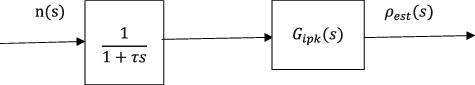
where τ is time constant of the filter.

This is the theoretically obtained transfer function of the reactivity meter based on IPK.

3.2. Simple feedback method (SRE)

Derivation of the transfer function of the reactivity meter based on SRE is discussed in the previous paper [1] as a part of the transfer function for input reactivity to output reactivity. The derivation of the transfer function for fluctuation of input neutron density to output reactivity is explained as follows. Again, a linearized version of the point kinetic model with one family of delayed neutron precursors is used.

The related equations for SRE reactivity meter are expressed as follows.

The linearized kinetic equations are expressed as Equations (29)(29) $$\frac{\mathrm{d}n\left(t\right)}{\mathrm{d}t}=-\frac{\beta }{\ell }n\left(t\right)+\lambda C\left(t\right)+\frac{\rho \left(t\right)}{\ell }{n}_0$$(29) and (30(30) $$\frac{\mathrm{d}C\left(t\right)}{\mathrm{d}t}=\frac{\beta }{\ell }n\left(t\right)-\lambda C\left(t\right).$$(30) ), of which input reactivity is ρ_est(t) and the output neutron density, n_exp(t). Thus, the kinetic equations are given as (39) $$\frac{\mathrm{d}{n}_{\exp }\left(t\right)}{\mathrm{d}t}=-\frac{\beta }{\ell }{n}_{\exp }\left(t\right)+\lambda C\left(t\right)+\frac{{\rho }_{\mathrm{est}}\left(t\right)}{\ell }{n}_0$$(39) (40) $$\frac{\mathrm{d}C\left(t\right)}{\mathrm{d}t}=\frac{\beta }{\ell }{n}_{\exp }\left(t\right)-\lambda C\left(t\right).$$(40)

Note that they are equations for the deviations from the initial values, omitting deviation sign of δ. The solution for these equations gives the expected neutron density, n_exp(t).

Then, the difference of the input neutron density, n(t), and the expected neutron density, n_exp(t), is given as (41) $$\delta n\left(t\right)=n\left(t\right)-n_{\exp }\left(t\right)$$(41)

The correction reactivity, δρ(t), is given as (42) $$\delta \rho \left(t\right)=K\delta n\left(t\right)$$(42)

Then the corrected reactivity, ρ_est(t), is given as the integration of δρ(t) as (43) $${\rho }_{\mathrm{est}}\left(t\right)=\underset{0}{\overset{t}{\int }}\delta \rho \left(\tau \right)\mathrm{d}\tau$$(43)

In order to derive transfer function of SRE, it is necessary to get the ratio of Laplace transformed reactivity output and the input neutron density. Thus, all of these equations are Laplace transformed. However, the solution for the Equations of (39(39) $$\frac{\mathrm{d}{n}_{\exp }\left(t\right)}{\mathrm{d}t}=-\frac{\beta }{\ell }{n}_{\exp }\left(t\right)+\lambda C\left(t\right)+\frac{{\rho }_{\mathrm{est}}\left(t\right)}{\ell }{n}_0$$(39) ) and (40(40) $$\frac{\mathrm{d}C\left(t\right)}{\mathrm{d}t}=\frac{\beta }{\ell }{n}_{\exp }\left(t\right)-\lambda C\left(t\right).$$(40) ) is given as (44) $$n_{\exp }\left(s\right)=G_R\left(s\right){\rho }_{\mathrm{est}}\left(s\right)$$(44)

The Laplace transformed equations for the rest of the equations are given as (45) $$\delta n\left(\mathrm{s}\right)=n\left(s\right)-n_{\exp }\left(s\right)$$(45) (46) $$\delta \rho \left(s\right)=K\delta n\left(s\right)$$(46) (47) $${\rho }_{\mathrm{est}}\left(s\right)=\frac{\delta \rho \left(s\right)}{s}.$$(47)

Substituting Equation (44)(44) $$n_{\exp }\left(s\right)=G_R\left(s\right){\rho }_{\mathrm{est}}\left(s\right)$$(44) into Equation (45)(45) $$\delta n\left(\mathrm{s}\right)=n\left(s\right)-n_{\exp }\left(s\right)$$(45) , (48) $$\delta n\left(s\right)=n\left(s\right)-G_R\left(s\right){\rho }_{\mathrm{est}}\left(s\right).$$(48)

Equation (48)(48) $$\delta n\left(s\right)=n\left(s\right)-G_R\left(s\right){\rho }_{\mathrm{est}}\left(s\right).$$(48) is substituted into Equation (46)(46) $$\delta \rho \left(s\right)=K\delta n\left(s\right)$$(46) to get (49) $$\delta \rho \left(s\right)=K\left(n\left(s\right)-G_R\left(s\right){\rho }_{\mathrm{est}}\left(s\right)\right)$$(49)

Substituting Equation (49)(49) $$\delta \rho \left(s\right)=K\left(n\left(s\right)-G_R\left(s\right){\rho }_{\mathrm{est}}\left(s\right)\right)$$(49) into Equation (47)(47) $${\rho }_{\mathrm{est}}\left(s\right)=\frac{\delta \rho \left(s\right)}{s}.$$(47) to get (50) $${\rho }_{\mathrm{est}}\left(s\right)=\frac{K\left(n\left(s\right)-G_R\left(s\right){\rho }_{\mathrm{est}}\left(s\right)\right)}{s}$$(50)

Solving for ρ_est(s), we get (51) $${\rho }_{\mathrm{est}}\left(s\right)=\frac{Kn\left(s\right)}{s+K{G}_R\left(s\right)}$$(51)

Substituting G_R(s) to Equation (51)(51) $${\rho }_{\mathrm{est}}\left(s\right)=\frac{Kn\left(s\right)}{s+K{G}_R\left(s\right)}$$(51) to get (52) $${\rho }_{\mathrm{est}}\left(s\right)=\frac{K\left(s\left(s\ell +\ell \lambda +\beta \right)\right)}{s^2\left(s\ell +\ell \lambda +\beta \right)+K\left(s+\lambda \right)n_0}n\left(s\right),$$(52) where ρ_est(s) is estimated reactivity, n (s) is input fluctuation of neutron density, K is feedback gain, G_R(s) is transfer function of the linearized point kinetic model, $$=\frac{s+\lambda }{s\left(\mathrm{s}\ell +\lambda \ell +\beta \right)}{n}_0$$and n₀ is initial neutron flux.

However, in this expression, a non-linear term, K, is included. Thus, we further simplify the model by assuming that the reactivity is close to zero, and thus the feedback gain, K, of Equation (19)(19) $$K=\frac{\beta -{\rho }_k}{n_{t,k+1}}.$$(19) can be expressed as (53) $$K=\frac{\beta }{n_{t,k+1}}.$$(53)

When the neutron flux is changing with a small amplitude around the initial value, then we can further simplify the feedback gain as (54) $$K=\frac{\beta }{n_0}.$$(54)

Then, Equation (51)(51) $${\rho }_{\mathrm{est}}\left(s\right)=\frac{Kn\left(s\right)}{s+K{G}_R\left(s\right)}$$(51) can be expressed as (55) $${\rho }_{\mathrm{est}}\left(s\right)=\frac{\frac{\beta }{n_0}}{\mathrm{s}+\frac{\beta }{n_0}\frac{\mathrm{s}+\lambda }{\mathrm{s}\left(\mathrm{s}\ell +\lambda \ell +\beta \right)}{\mathrm{n}}_0}n\left(s\right).$$(55)

Thus, the transfer function can be expressed as (56) $$G_{\mathrm{sre}}\left(s\right)\mathit{}=\frac{{\rho }_{\mathrm{est}}}{n\left(s\right)}=\frac{\beta s\left(\mathrm{s}\ell +\lambda \ell +\beta \right)}{s^2\left(s\ell +\lambda \ell +\beta \right)+\beta \left(s+\lambda \right)}\frac{1}{n_0}.$$(56)

In order to filter noise components from the reactivity, it is necessary to adjust the feedback gain using a gain adjuster F as follows:(57) $$\delta \rho =F\frac{\beta -{\rho }_k}{n_{t,k+1}}\delta n.$$(57)

Taking the adjustment into account, Equation (54)(54) $$K=\frac{\beta }{n_0}.$$(54) can be expressed as (58) $$K=F\frac{\beta }{n_0}.$$(58)

Then Equation (56)(56) $$G_{\mathrm{sre}}\left(s\right)\mathit{}=\frac{{\rho }_{\mathrm{est}}}{n\left(s\right)}=\frac{\beta s\left(\mathrm{s}\ell +\lambda \ell +\beta \right)}{s^2\left(s\ell +\lambda \ell +\beta \right)+\beta \left(s+\lambda \right)}\frac{1}{n_0}.$$(56) is rewritten as (59) $$G_{\mathrm{sre}}\left(s\right)=\frac{F\beta s\left(s\ell +\ell \lambda +\beta \right)}{s^2\left(s\ell +\ell \lambda +\beta \right)+F\beta \left(s+\lambda \right)}\frac{1}{n_0}.$$(59)

The system diagram for this reactivity meter is shown in Figure 2.

Figure 2. Block diagram of SRE.

As can be seen, this transfer function is based on linearized kinetic equations, and moreover, the feedback gain is approximated as constant. This implies that the discussion is valid for a small reactivity perturbation. However, in the actual application, the feedback gain is not constant but depending on the neutron density as in Equation (19)(19) $$K=\frac{\beta -{\rho }_k}{n_{t,k+1}}.$$(19) , which can result in accurate reactivity estimation even with large reactivity change as shown in reference [1].

One more thing to be noted is that the analysis based on transfer function treats problems in continuous time domain, however, in the digital reactivity meters, calculations are done in discretized time domain. Thus, the relation of F and τ can change according to calculation time interval.

Now the analytical expressions of the transfer functions for the two reactivity meters are obtained on the same theoretical modeling. Thus, we can discuss the comparison of performance on the same basis.

The reactor kinetic parameters used in the analyses are listed in Table 1, which are typical values for light water reactors.

Table 1. Reactor kinetic parameters.

Delayed neutron fraction	0.0065
Delayed neutron precursors decay constant	0.078 sec^−1
Prompt neutron life time	0.00002 sec

4. Comparison of performance and correlation of system parameters of the two reactivity meters

The performance of the reactivity meters depends on the respective system parameter, i.e. the time constant, τ, for IPK and the gain adjustment, F, for SRE. These parameters control the time response of the estimated reactivity and the time response is directly related with the capability of noise filtering as discussed in reference [6]. Thus, it is important to evaluate how performance depends on these system parameters. From this point of view, the calculated reactivity difference between IPK and SRE is compared for the same input.

The procedures are as follows. Neutron density transient, n(s), is obtained as the product of G_R(s) and input reactivity, ρ(s). Estimated reactivity by the reactivity meter based on IPK and SRE is obtained as the product of n(s) and respective transfer functions of G_ipk(s) and G_sre(s). The reactivity difference between those obtained by the two reactivity meters, R_diff(s), is expressed as follows: (60) $$\begin{array}{ccc}\hfill R_{\mathrm{diff}}\left(s\right)& =& \left(G_{\mathrm{ipk}}\left(s\right)-G_{\mathrm{sre}}\left(s\right)\right)n\left(s\right)\hfill \\ & =& \left(G_{\mathrm{ipk}}\left(s\right)-G_{\mathrm{sre}}\left(s\right)\right)G_R\left(s\right)\rho \left(s\right).\hfill \end{array}$$(60)

Now it is possible to evaluate the correlation between τ and F to minimize this reactivity difference.

However, the above expression is not in the time domain. It is necessary to inversely Laplace transform to evaluate the difference in time domain. The reactivity response expressions in time domain are obtained using a powerful capability of inverse Laplace transformation by Wolfram's Mathematica-11 [9]. The correlation for τ and F to minimize the difference is investigated numerically.

Typical reactivity difference defined in Equation (60)(60) $$\begin{array}{ccc}\hfill R_{\mathrm{diff}}\left(s\right)& =& \left(G_{\mathrm{ipk}}\left(s\right)-G_{\mathrm{sre}}\left(s\right)\right)n\left(s\right)\hfill \\ & =& \left(G_{\mathrm{ipk}}\left(s\right)-G_{\mathrm{sre}}\left(s\right)\right)G_R\left(s\right)\rho \left(s\right).\hfill \end{array}$$(60) is shown in Figure 3. The sign of the difference may change with time. Thus, the square of the difference is integrated for the 50 sec after the initiation of the transient to find out whether or not there is a setting of τ and F that gives the minimum difference, or in other words, the identical performance for both reactivity meters. For this evaluation, a step reactivity of 0.005 is added.

Figure 3. Typical reactivity difference.

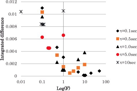
The numerical results are shown in Table 2 for the combinations of the system parameters focusing in the area of interest, that is, the results are focused in the vicinity of the F values to give the minimum value of the integration. The system parameter, τ, is ranging from 0.1 to 10 sec which are selected considering the actual application. The results are shown in Figure 4. As can be seen in Figure 4, it is clear that the minimum integrations are located in close range of F for respectiveτ. In other words, when the system parameters satisfy the correlation of Fτ = 1.0, the integration become the minimum value. For some cases (F = 0.11; τ = 10.0 sec and F = 0.21; τ = 5.0 sec), the correlation does not apply, however, the deviation of the integration is quite small.

Table 2. Numerical results of the integrated square of the reactivity difference.

F	τ = 0.1 sec	τ = 0.5 sec	τ = 1.0 sec	τ = 5.0 sec	τ = 10 sec
0.01					0.014020
0.09					0.008408
0.1	0.010994	0.010346	0.009587	0.006286	0.008345
0.11					0.008327
0.12					0.008342
0.19				0.004535
0.2				0.004518
0.21				0.004516
0.22				0.004525
0.5	0.004640	0.003381	0.002241
0.9			0.001007
1	0.003040	0.001518	0.000970	0.006601	0.01053
1.1			0.000996
2		0.000491
3		0.000805
5	0.000657	0.001345	0.002682
9	0.000134
10	0.000103	0.001866	0.003087
11	0.000127
20	0.000471
50	0.000830

Figure 4. Comparison of the integrated square of the reactivity difference.

It should be pointed out that the integration is carried out for the square of the reactivity difference over the time interval of 50 sec after the neutron density fluctuation is given. Thus, the minimum integration means that the time response and the reactivity of the two reactivity meters are very close. In other words, when the time response is different, the integration becomes large even if the reactivity difference is small. When the reactivity difference is large, the integration also becomes large. It can be seen in the following figures.

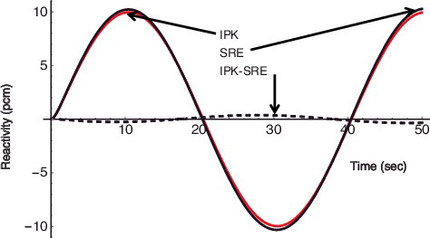
Some examples of reactivity transients are shown in Figures 5–7 for a step reactivity of 10 pcm, a ramp reactivity of 0.05 pcm/sec, and a sinusoidal reactivity of 10 pcm × s$\mathrm{in}\left(\frac{\pi }{20t}\right)$, respectively. It can be seen that the difference of the reactivity estimation between the two reactivity meters is quite small in comparison with the criteria of plus or minus 4% of relative error for recalibration of reactivity meter. Note that a pcm means 10^{− 5} of reactivity.

Figure 5. Reactivity response for a step reactivity input of 10 pcm τ = 0.5 sec for IPK and F = 2.0 for SRE.

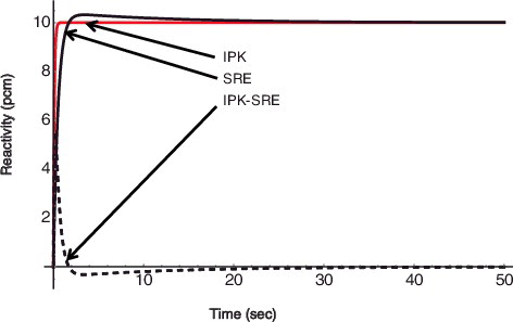
Figure 6. Reactivity response for a ramp reactivity input for 0.5 pcm/sec τ = 0.5 sec for IPK and F = 2.0 for SRE.

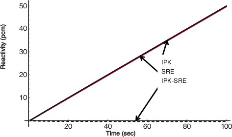
Figure 7. Reactivity response for a sinusoidal reactivity input of 10 pcm × sin(π/20t); τ = 0.5 sec for IPK and F = .0 for SRE.

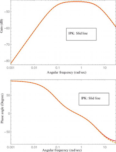
The filtering characteristics and time response can be also evaluated by frequency response. Bode charts for the two reactivity meters are compared for the system parameters with correlation of Fτ = 1.0, for example, τ = 1(sec) and F = 1.0 in Figure 8. It can be seen that the frequency responses of the two transfer functions are identical. In other words, from the gain chart, the noise-filtering characteristics are known. From the phase chart, time response capability is known. As both the frequency responses are identical, it can be concluded that both the reactivity meters can be identical under certain system parameter settings in noise filtering and time response. In other words, the newly proposed SRE reactivity meters can be used in actual reactor systems with the same reliability as IPK reactivity meters. Changing the system parameter, F, has the same effect as to changing the system parameter, τ, in IPK reactivity meters. The above correlation is quite useful to select system parameter for respective reactivity meter based on the performance of the other one.

Figure 8. Comparison of Bode charts for IPK and SRE transfer functions; τ = 0.5 sec and F = 2.0.

The reason that the minimum reactivity difference is obtained with the correlation of Fτ = 1.0 can be explained as follows. Using the reactor transfer function, G_R(s) of Equation (37)(37) $$G_R\left(s\right)=\frac{n\left(s\right)}{{\rho }_{\mathrm{est}}\left(s\right)}=\frac{s+\lambda }{s\left(s\ell +\lambda \ell +\beta \right)}{n}_0$$(37) , Equation (60)(60) $$\begin{array}{ccc}\hfill R_{\mathrm{diff}}\left(s\right)& =& \left(G_{\mathrm{ipk}}\left(s\right)-G_{\mathrm{sre}}\left(s\right)\right)n\left(s\right)\hfill \\ & =& \left(G_{\mathrm{ipk}}\left(s\right)-G_{\mathrm{sre}}\left(s\right)\right)G_R\left(s\right)\rho \left(s\right).\hfill \end{array}$$(60) is written as (61) $$R_{\mathrm{diff}}=\left(\frac{1}{1+\tau s}-\frac{F\beta G_R\left(s\right)}{s{n}_0+F\beta G_R\left(s\right)}\right)\rho \left(s\right).$$(61)

This equation is further re-written as (62) $$\begin{array}{ccc}\hfill R_{\mathrm{diff}}& =& \left(\frac{1}{1+\tau s}-1+\frac{s{n}_0}{s{n}_0+F\beta G_R\left(s\right)}\right)\hfill \\ \hfill \rho \left(s\right)& =& \left(\frac{1}{1+\tau s}-1\right)\rho \left(s\right)+\frac{s{n}_0}{s{n}_0+F\beta G_R\left(s\right)}\rho \left(s\right).\hfill \end{array}$$(62)

For a step input reactivity of 0.005, the reactivity difference is expressed as (63) $$R_{\mathrm{diff},0.005\mathrm{step}}=\left(\frac{1}{1+\tau s}-1\right)\frac{0.005}{s}+\frac{0.005n_0}{s{n}_0+F\beta G_R\left(s\right)}.$$(63)

The first term on the right side of Equation (62)(62) $$\begin{array}{ccc}\hfill R_{\mathrm{diff}}& =& \left(\frac{1}{1+\tau s}-1+\frac{s{n}_0}{s{n}_0+F\beta G_R\left(s\right)}\right)\hfill \\ \hfill \rho \left(s\right)& =& \left(\frac{1}{1+\tau s}-1\right)\rho \left(s\right)+\frac{s{n}_0}{s{n}_0+F\beta G_R\left(s\right)}\rho \left(s\right).\hfill \end{array}$$(62) gives the reactivity difference obtained by subtracting the input reactivity from the reactivity of IPK. As can be seen, the reactivity meter gives a response with a time delay of τ. The second term on the right side of Equation (62)(62) $$\begin{array}{ccc}\hfill R_{\mathrm{diff}}& =& \left(\frac{1}{1+\tau s}-1+\frac{s{n}_0}{s{n}_0+F\beta G_R\left(s\right)}\right)\hfill \\ \hfill \rho \left(s\right)& =& \left(\frac{1}{1+\tau s}-1\right)\rho \left(s\right)+\frac{s{n}_0}{s{n}_0+F\beta G_R\left(s\right)}\rho \left(s\right).\hfill \end{array}$$(62) gives the reactivity difference subtracting SRE reactivity from the input reactivity. This can be seen from the following equation. SRE reactivity is given as (64) $$\begin{array}{ccc}\hfill G_{\mathrm{sre}}\left(s\right)G_R\left(s\right)\rho \left(s\right)& =& \frac{F\beta G_R\left(s\right)}{s{n}_0+F\beta G_R\left(s\right)}\hfill \\ \hfill \rho \left(s\right)& =& \left(1-\frac{s{n}_0}{s{n}_0+F\beta G_R\left(s\right)}\right)\rho \left(s\right).\hfill \end{array}$$(64)

Thus, (65) $$\frac{s{n}_0}{s{n}_0+F\beta G_R\left(s\right)}\rho \left(s\right)=\left(1-\frac{F\beta G_R\left(s\right)}{s{n}_0+F\beta G_R\left(s\right)}\right)\rho \left(s\right).$$(65)

Note that as G_R(s) includes n₀ component, n₀ is canceled in both denominator and numerator in Equation (65)(65) $$\frac{s{n}_0}{s{n}_0+F\beta G_R\left(s\right)}\rho \left(s\right)=\left(1-\frac{F\beta G_R\left(s\right)}{s{n}_0+F\beta G_R\left(s\right)}\right)\rho \left(s\right).$$(65) , thus, Equation (65)(62) $$\begin{array}{ccc}\hfill R_{\mathrm{diff}}& =& \left(\frac{1}{1+\tau s}-1+\frac{s{n}_0}{s{n}_0+F\beta G_R\left(s\right)}\right)\hfill \\ \hfill \rho \left(s\right)& =& \left(\frac{1}{1+\tau s}-1\right)\rho \left(s\right)+\frac{s{n}_0}{s{n}_0+F\beta G_R\left(s\right)}\rho \left(s\right).\hfill \end{array}$$(62) is independent on n₀.

The behavior of both the terms of Equation (62)(62) $$\begin{array}{ccc}\hfill R_{\mathrm{diff}}& =& \left(\frac{1}{1+\tau s}-1+\frac{s{n}_0}{s{n}_0+F\beta G_R\left(s\right)}\right)\hfill \\ \hfill \rho \left(s\right)& =& \left(\frac{1}{1+\tau s}-1\right)\rho \left(s\right)+\frac{s{n}_0}{s{n}_0+F\beta G_R\left(s\right)}\rho \left(s\right).\hfill \end{array}$$(62) is inversely Laplace transformed and compared in Figure 9.

Figure 9. Comparison of the respective reactivity difference for IPK and SRE.

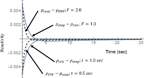
As can be seen in this comparison, both the terms show quite similar transient with the inverse signs only when the correlation Fτ = 1.0. This explains the reason to give the minimum reactivity difference. It is clear that the reactivity difference is dependent on the transient behavior of reactivity of each reactivity meter. It means that the physical meaning of F in SRE corresponds to τ for IPK even if the transfer functions do not look alike.

Additional discussion is given for the application of SRE in a digital system. As is known for the analysis in transfer functions, all the state variables are initially set to be zero. Thus, in SRE, reactivity is corrected in time continuous system using feedback logic. However, in a discretized digital system, the reactivity correction is done in one step. Thus, the feedback effect is direct. This causes the slower time response by transfer function of SRE than by a digital system. Based on our experiences, the time response can be compensated by increasing the F value in transfer function by 10 times to obtain the same response by digital system. However, the adjustment may be optional by the designers considering the environment of the application. The other notice is that in the actual application the non-linearity characteristics are correctly taken into account as discussed in Section 2.

It is pointed out that the difference between IPK and SRE performance is that the former performance is fixed when a time delay has been selected. However, the latter can adjust the performance by adjusting F according to the neutron flux level discussed in reference [1]. Thus, in actual application, the result of this paper can be used practically as follows. Select a proper value of F considering the noise level at the initial condition to corresponding IPK reactivity. Note that the neutron flux is normalized to this initial value in SRE reactivity meter. Normally, the initial condition is expected as that when the neutron flux is relatively high in comparison with noise. With this setting, SRE is suitable for monitoring reactivity under sub-critical conditions when the neutron density decreases more than 2 decades from the initial value as discussed in the reference [1].

5. Conclusion

The reactivity outputs from both IPK and SRE reactivity meters are compared using respective theoretical transfer functions, by varying time constant, τ of the first-order delay filter in IPK reactivity meter and the gain adjuster F in SRE reactivity meter. With this result and discussion of theoretical comparison, the characteristics of F become clear that the physical meaning of F in SRE corresponds to τ for IPK even if the transfer functions do not look alike. It becomes clear that when the product of the time constant in IPK and the gain adjuster, F, for SRE equals to unity, i.e. Fτ = 1.0, the performance of both reactivity meters is identical, which means that they show the same noise-filtering and time response capability. In other words, the SRE reactivity meters can be used in the actual reactor systems in the same manner as the conventional IPK reactivity meters. These two parameters are the key parameter to each of the reactivity meter. With this correlation, filter designers can easily determine the system parameters for the respective reactivity meters to obtain identical performance suitable for the environment of neutron flux signal. However, SRE can provide better noise-filtering capability than IPK owing to its robust filter especially under environment with quite low neutron density with high noise fraction.

Acknowledgments

The authors express sincere gratitude to Dr W.F.G. van Rooijen of the Research Institute of Nuclear Engineering, University of Fukui, Japan for his assistance in the preparation of this manuscript.

A part of this study is the result of ‘Development of sub-criticality monitoring method during shutdown and refueling modes of nuclear power plant operation’ carried out under the Center of World Intelligence Project for Nuclear S&T and Human Resource Development by the Ministry of Education, Culture, Sports, Science and Technology of Japan [grant number 271105].

Disclosure statement

No potential conflict of interest was reported by the authors.

Additional information

Funding

the Ministry of Education, Culture, Sports, Science and Technology of Japan

References

- Shimazu Y. A simple procedure to estimate reactivity with good noise filtering characteristics. Ann Nucl Energy. 2014;73:392–397.
- Shimazu Y, Unesaki H, Suzuki N. Subcriticality monitoring with a digital reactivity meter. J Nucl Sci Technol. 2003;40:970–974.
- Naing W, Tsuji M, Shimazu Y. Subcriticality measurement of pressurized water reactor during criticality approach using a digital reactivity meter. J Nucl Sci Technol. 2005;42:145–152.
- Shimazu Y, Naing W. Some technical issues on continuous subcriticality monitoring by a digital reactivity meter during criticality approach. J Nucl Sci Technol. 2005;42:515–524.
- Shimazu Y, Naing W, Tsuji M. Feasibility study of continuous subcriticality monitoring using a digital reactivity meter to overcome the criticality accident. J Nucl Sci Technol. 2006;43:1414–1421.
- Shimazu Y, Rooijen WFG. Qualitative performance comparison of reactivity estimation between the extended Kalman filter technique and the inverse point kinetic method. Ann Nucl Energy. 2014;66:161–166.
- Shimazu Y, Nakano Y, Tahana y, et al. Development of a digital reactivity meter and a reactor physics data processor. Nucl Technol. 1987;77(6):247–254.
- Bell GI, Glasstone S. Nuclear reactor theory. 1st ed. New York (NY): Van Nostrand Reinhold Company; 1970. p. 480–482.
- Mathematica [CD-ROM]. Version 11. Champaign (IL): Wolfram Resaerch, Inc.; 2016.