Estimation of sensitivity coefficient based on lasso-type penalized linear regression

ABSTRACT

We proposed the penalized regression ‘adaptive smooth-lasso’ for the estimation of sensitivity coefficients of the neutronics parameters. The proposed method utilizes the variation of the microscopic cross-sections and the neutronics parameters obtained by random sampling. The weighted penalty term of the proposed method is more appropriate for the estimation of the sensitivity of neutronics parameters to the microscopic cross-section than that of the conventional methods. In a numerical verification calculation, sensitivity coefficients of k_eff of an accelerator-driven system are estimated using the proposed method, the conventional penalized regression, and the direct method. Comparison of these results indicates that the proposed method is superior to the conventional penalized linear regression from the viewpoint of reproduction of the reference sensitivity coefficients obtained by the direct method. Through the verification calculations, the proposed method can be a candidate for a practical method to estimate the sensitivity coefficients with low calculation cost.

KEYWORDS:

• Sensitivity coefficient
• random sampling
• L1 norm
• lasso
• penalized linear regression

View correction statement:

Correction

1. Introduction

For the safe and efficient operation of nuclear reactors, it is important to quantify and reduce the uncertainty of core neutronics parameters predicted by numerical core analysis. In addition, the uncertainties propagated from the nuclear data are still large for a future nuclear system such the accelerator-driven system (ADS); thus, both of the differential and integral experiment data for efficient reduction of the uncertainties of the design calculations are desirable. The identification of the dominant nuclear data for uncertainties is important to propose the desired experiment. The sensitivity coefficients of the core neutronics parameter to cross-section data are often used for uncertainty quantification based on error propagation, cross-section adjustment method, and a method to identify nuclear data for which further improvements are required to reduce uncertainties of target integral neutronics parameters [1–3]. Consequently, evaluation of the sensitivity coefficients of core neutronics parameters is important in core analysis.

There are several sensitivity estimation methods, e.g. the forward method, the adjoint method, and the method based on reduced order modeling (ROM). The forward method estimates the sensitivity coefficients by performing the perturbed calculations for each input parameter. The forward method can utilize the existing codes without major modifications; thus, the use of the forward method is very easy. However, the calculation cost of this method is proportional to the number of input parameters taken into account; thus, this method would be impractical due to a large number of input parameters (e.g. fine-group microscopic cross-sections). On the other hand, in the adjoint method, the adjoint models defined for each interesting neutronics parameters are evaluated to estimate the sensitivity coefficients [4–6]. The calculation cost of this method is independent of the number of input parameters. Thus, when the number of the neutronics parameters is less than that of the input parameters, the adjoint method is superior to the forward method from the viewpoint of the calculation cost. However, the adjoint method generally requires modification of the calculation code system to solve the adjoint model. It would require a great effort to modify the complicated code system which performs the series of core analysis by combining several codes (e.g. lattice-calculation, core-calculation, and burnup-calculation codes) and the definition of the adjoint model for such a complicated code system will be sometimes difficult. Thus, the application of the adjoint method would be difficult to perform. Furthermore, the calculation cost of the adjoint method is proportional to the number of the neutronics parameters taken into account; thus, the adjoint method would be also impractical when the number of the neutronics parameters (e.g. power distribution, space/energy flux distribution, and the number density of the nuclides) is large. In ROM approach, the neutronics and/or input parameters are expanded in the active subspace (AS), which can well express the variation of the parameters with fewer dimensions than that of the original parameters space. With the expansion, the effective number of parameters can be significantly reduced; thus, the calculation cost can be also reduced. The various methods are proposed to construct the AS in the previous study [7–11].

As another approach, the previous studies proposed the method based on random sampling [12,13]. These methods estimate the sensitivity coefficients by solving the simultaneous linear equations whose solution is the sensitivity coefficients. The calculation cost of these methods is proportional to the number of the random samples, although these methods utilize only forward calculations. Therefore, the calculation cost is less than that of the forward method when the number of samples is smaller than that of the microscopic cross-sections. However, in such case, the simultaneous equation for the sensitivity coefficients is an underdetermined system (as described in Section 2.1); thus, the constraint condition is required. In Ref. [13], the sensitivity coefficients are determined based on the L1 norm minimization. Generally, the solution obtained by the L1 norm minimization is sparse; most of the elements of which are zero [14]. In typical reactor analysis, most of the cross-sections have a very small impact on neutronics parameters (i.e. small sensitivity coefficient) and a small part of cross-section dominates neutronics parameters (i.e. large sensitivity coefficient). In other words, sensitivity coefficients for cross-sections are very ‘sparse’. Consequently, the L1 norm minimization can adequately estimate especially large sensitivity coefficients with the smaller number of the random samples than that of the input parameters [13]. As a similar approach, the penalized linear regression ‘lasso’, in which the L1 norm of the solution vector is considered as the penalized term, is proposed [15]. Lasso can obtain the sparse solution similar to the L1 norm minimization method. However, in the L1 norm minimization and lasso methods, it is assumed that the cross-section to which sensitivity coefficient is zero is unknown. Thus, the non-zero sensitivity coefficients are sometimes evaluated as zero, and vice versa.

Now, let us consider the shape of sensitivity coefficients. The energy region of large sensitivity coefficients depends on the type of a reactor, e.g. thermal or fast reactor. For instance, in a fast reactor, the sensitivity coefficients have large positive or negative values in fast energy region and have very small values in thermal energy region. Namely, the non-zero elements of the sensitivity coefficients are not randomly distributed but are clustered in a certain energy region depending on the type of reactor. Therefore, we focus on the ‘smooth-lasso’ whose penalized term consists of not only the L1 norm but also the sum of squares of the difference between adjacent elements [16]. The smooth-lasso can select the solution that is sparse but the difference between adjacent elements is small. It means that the elements show smooth change for the index of the solution vector. Owing to the smoothness, zero and non-zero elements of a solution vector selected by smooth-lasso would be clustered, respectively. Therefore, the smooth-lasso would be more appropriate for the estimation of the sensitivity coefficients than the lasso. However, the sensitivity coefficients would not change smoothly depending on the energy range due to the threshold reactions and the giant resonance cross-sections, although the non-zero elements are distributed in a cluster in certain energy region. Thus, in this paper, we propose the weighted penalized linear regression ‘adaptive smooth-lasso’ that would be more appropriate for the estimation of sensitivity coefficients of the neutronics parameters to the microscopic cross-sections than the lasso and smooth-lasso. The main objective of this paper is to confirm the applicability of the adaptive smooth-lasso compared to the two conventional methods, i.e. the lasso and the smooth-lasso. In this paper, we evaluate the applicability of the adaptive smooth-lasso through estimation of the sensitivity coefficients of the effective multiplication factor k_eff of an ADS.

This paper is organized as follows. In Section 2, estimation of the sensitivity coefficients based on the random sampling and the penalized linear regression is described. In Section 3, numerical results of the proposed method are shown in comparison with the conventional and the direct methods. Finally, concluding remarks are summarized in Section 4.

2. Theory

2.1. Penalized regression in random-sampling of cross-section

First, we consider that the numbers of the cross-sections, the neutronics parameters, and the samples are $N$, one, and $M$, respectively. Using the first-order approximation of the Taylor expansion, relative variation of a neutronics parameters obtained with small relative variations of the cross-sections is approximately expressed as follows:

(1) $\mathrm{\Delta }{R}_i=\sum _{j=1}^N\mathrm{\Delta }{T}_{ij}{g}_j,$(1)

where $i$ is the index of the sample, $j$ is the index of the cross-sections, $\mathrm{\Delta }{R}_i$ is relative variation of the neutronics parameter in the $i$-th sample, $\mathrm{\Delta }{T}_{ij}$ is relative variation of the $j$-th cross-section in the $i$-th sample, and $g_j$ is the relative sensitivity coefficient of the neutronics parameter to the $j$-th cross-section ($g_j\equiv \left(dR/R\right)/\left(d{T}_j/T_j\right)$). Equation (1)(1) $\mathrm{\Delta }{R}_i=\sum _{j=1}^N\mathrm{\Delta }{T}_{ij}{g}_j,$(1) can be represented in a matrix-vector form as follows:

(2) $\mathrm{\Delta }\vec{R}=\mathrm{\Delta }\mathbf{T}\vec{g},$(2)

where, $\mathrm{\Delta }\vec{R}$, $\mathrm{\Delta }\mathbf{T}$, and $\vec{g}$ can be written as follows:

(3) $\mathrm{\Delta }\vec{R}={\left(\mathrm{\Delta }{R}_1,\mathrm{\Delta }{R}_2,\dots ,\mathrm{\Delta }{R}_M\right)}^T,$(3)

(4) $\mathrm{\Delta }T=\left(\begin{array}{cccc}\mathrm{\Delta }{T}_{11}& \mathrm{\Delta }{T}_{12}& \dots & \mathrm{\Delta }{T}_{1N}\\ \mathrm{\Delta }{T}_{21}& \mathrm{\Delta }{T}_{22}& \dots & \mathrm{\Delta }{T}_{2N}\\ ⋮& ⋮& \ddots & ⋮\\ \mathrm{\Delta }{T}_{M1}& \mathrm{\Delta }{T}_{M2}& \dots & \mathrm{\Delta }{T}_{MN}\end{array}\right),$(4)

(5) $\vec{g}={\left(g_1,g_2,\dots ,g_N\right)}^T.$(5)

$\mathrm{\Delta }\vec{R}$, $\mathrm{\Delta }\mathbf{T}$, and $\vec{g}$ are $M$-dimensional vector, $M$-by-$N$ matrix, and $N$-dimensional vector, respectively. In the estimation of the sensitivity coefficients, Equation (2)(2) $\mathrm{\Delta }\vec{R}=\mathrm{\Delta }\mathbf{T}\vec{g},$(2) is a simultaneous linear equation whose solution is the vector $\vec{g}$. When $M$ < $N$, the number of equations is fewer than that of unknowns (i.e. elements of $\vec{g}$) so the solution of Equation (2)(2) $\mathrm{\Delta }\vec{R}=\mathrm{\Delta }\mathbf{T}\vec{g},$(2) cannot be uniquely determined. For such the underdetermined system, the solution $\vec{g}$ can be determined by the penalized linear regression as follows [17]:

(6) $\vec{g}=\mathrm{a}\mathrm{r}\mathrm{g}\mathrm{m}\mathrm{i}\mathrm{n}\left\{\frac{1}{2}\sum _{i=1}^M{\left(\mathrm{\Delta }{R}_i-\sum _{j=1}^N\mathrm{\Delta }{T}_{ij}{g}_j\right)}^2+p\left(\vec{g}\right)\right\},$(6)

where, $p\left(\vec{g}\right)$ is the penalty term and the argmin of a function is the values of the arguments at which the function is minimized. The various types of the penalty term are proposed as follows: [17]:

(7) $p\left(\vec{g}\right)=\frac{\lambda }{2}\sum _{j=1}^N{g}_j^2,$(7)

(8) $p\left(\vec{g}\right)=\lambda \sum _{j=1}^N\left|g_j\right|,$(8)

(9) $p\left(\vec{g}\right)={\lambda }_1\sum _{j=1}^N\left|g_j\right|+\frac{{\lambda }_2}{2}\sum _{j=2}^N{\left(g_j-g_{j-1}\right)}^2,$(9)

where the regressions by Equation (7)(7) $p\left(\vec{g}\right)=\frac{\lambda }{2}\sum _{j=1}^N{g}_j^2,$(7) through Equation (9)(9) $p\left(\vec{g}\right)={\lambda }_1\sum _{j=1}^N\left|g_j\right|+\frac{{\lambda }_2}{2}\sum _{j=2}^N{\left(g_j-g_{j-1}\right)}^2,$(9) are called the ridge, lasso, and smooth-lasso, respectively. The parameters $\lambda$, ${\lambda }_1$ and ${\lambda }_2$ in Equation (7)(7) $p\left(\vec{g}\right)=\frac{\lambda }{2}\sum _{j=1}^N{g}_j^2,$(7) through Equation (9)(9) $p\left(\vec{g}\right)={\lambda }_1\sum _{j=1}^N\left|g_j\right|+\frac{{\lambda }_2}{2}\sum _{j=2}^N{\left(g_j-g_{j-1}\right)}^2,$(9) are user-defined tuning parameters. Equation (6)(6) $\vec{g}=\mathrm{a}\mathrm{r}\mathrm{g}\mathrm{m}\mathrm{i}\mathrm{n}\left\{\frac{1}{2}\sum _{i=1}^M{\left(\mathrm{\Delta }{R}_i-\sum _{j=1}^N\mathrm{\Delta }{T}_{ij}{g}_j\right)}^2+p\left(\vec{g}\right)\right\},$(6) determines $\vec{g}$ which minimizes the summation of the residual sum of squares between $\mathrm{\Delta }\vec{R}$ and $\mathrm{\Delta }\mathbf{T}\vec{g}$, and the penalty term depending on $\vec{g}$. The penalty term prohibits a solution whose elements are inappropriately large (e.g. point at infinity).

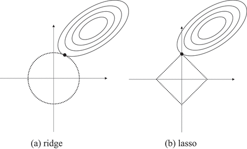
Figure 1 illustrates a difference between a solution by the ridge and the lasso. Figure 1 is a two-dimensional figure; however, each axis is corresponding to $g_1,g_2,\dots ,g_N$. The ellipses in Figure 1 represent contours which have the same residual sum of squares term, and the inner lines correspond to the smaller residual. Furthermore, the circle and the square centered at the origin represent the contour of the penalty term for the ridge and the lasso ($p\left(\vec{g}\right)$ = const), respectively. The contact point of the ellipse and contour of the penalty term is the solution which reduces both of the residual sum of squares and the penalty term. As shown in Figure 1, the lasso solution tends to locate at a corner, which contains a zero coefficient. On the other hands, no corner exists in the ridge penalty term thus the sparse solutions are rarely selected. The sensitivity coefficients of the neutronics parameters to the multi-group microscopic cross-sections are generally sparse; hence, the lasso will be appropriate to the estimation of the sensitivity coefficients.

Figure 1. Illustration of (a) the ridge and (b) lasso regressions. R. Katano: Estimation of sensitivity coefficient based on lasso-type penalized linear regression.

The penalty term of the smooth-lasso is defined as the sum of squares of the difference between adjacent elements. Therefore, the smooth-lasso selects the solution whose adjacent elements have the close values while keeping the sparsity. Namely, the zero and non-zero elements of the solution obtained by smooth-lasso would be distributed in a cluster while the lasso does not consider the structure of the non-zero elements. The large sensitivity coefficients of the neutronics parameters to the microscopic cross-sections are distributed in certain energy region depending on the type of reactor; thus, the smooth-lasso is expected more appropriate for the estimation of the sensitivity coefficients than the lasso. However, the elements of the solution obtained by smooth-lasso change smoothly depending on the energy index. Thus, the solution obtained by smooth-lasso would fail to reproduce the rapid changes of sensitivity coefficient due to threshold reactions or giant resonance cross-sections.

2.2. Adaptive smooth-lasso

As mentioned in the previous section, the solution obtained by the smooth-lasso would not sufficiently reproduce steep energy dependence of the sensitivity coefficients. Thus, we propose the weighted penalized regression ‘adaptive smooth-lasso’. The penalty term of the adaptive smooth-lasso is defined as follows:

(10) $p\left(\vec{g}\right)={\lambda }_1\sum _{j=1}^N{v}_j\left|g_j\right|+\frac{{\lambda }_2}{2}\sum _{j=2}^N{w}_j{\left(g_j-g_{j-1}\right)}^2.$(10)

Equation (10)(10) $p\left(\vec{g}\right)={\lambda }_1\sum _{j=1}^N{v}_j\left|g_j\right|+\frac{{\lambda }_2}{2}\sum _{j=2}^N{w}_j{\left(g_j-g_{j-1}\right)}^2.$(10) represents the penalty term of smooth-lasso multiplied by the weight $v_j$ and $w_j$. Here the weight $v_j$ and $w_j$ are defined as follows:

(11) $v_j=\frac{1}{1+c{\left|{\tilde{g}}_j\right|}^{\gamma }},$(11)

(12) $w_j=\frac{1}{1+c{\left(\frac{\left|{\tilde{g}}_j\right|+\left|{\tilde{g}}_{j-1}\right|}{2}\right)}^{\gamma }}.$(12)

The element $\tilde{g}$, and the constants $c$ and $\gamma$ represent the sensitivity coefficient estimated by smooth-lasso, and user-defined tuning parameters ($c$ > 0 and $\gamma$ > 0), respectively. As can be seen in Equations (11)(11) $v_j=\frac{1}{1+c{\left|{\tilde{g}}_j\right|}^{\gamma }},$(11) and (12(12) $w_j=\frac{1}{1+c{\left(\frac{\left|{\tilde{g}}_j\right|+\left|{\tilde{g}}_{j-1}\right|}{2}\right)}^{\gamma }}.$(12) ), the range of weight $v_j$ and $w_j$ is 0–1. These weights (i.e. $v_j$ and $w_j$) take small values for the large absolute values of the non-zero elements of the sensitivity coefficients obtained by smooth-lasso (i.e. ${\tilde{g}}_j$ or ${\tilde{g}}_{j-1}$). As the smaller values of the weight $v_j$, the L1 norm penalty term gets smaller. Thus, the $j$-th sensitivity coefficient $g_j$ tends to take a larger absolute value. Furthermore, as the smaller values of the weight $w_j$, the penalty term of the sum of squares of difference between adjacent elements gets smaller. Thus, the large difference between the adjacent elements (i.e. steep changes between ${\tilde{g}}_{j-1}$ and ${\tilde{g}}_j$) is allowed. Namely, it is expected that the adaptive smooth-lasso can emphasize the non-zero elements and allow the steep changes between the adjacent elements than the smooth-lasso. For zero elements, the weight still remains one; thus, zero element distribution would be similar between the smooth-lasso and adaptive smooth-lasso. As the larger value of $c$, the weights $v_j$ and $w_j$ take smaller values. As the smaller value of $\gamma$, the weights $v_j$ and $w_j$ take small values for smaller non-zero elements.

The adaptive smooth-lasso requires four user-defined tuning parameters, i.e. ${\lambda }_1$, ${\lambda }_2$, $c$, and $\gamma$. For example, when c is zero, the adaptive smooth-lasso is equivalent to the smooth-lasso. When ${\lambda }_2$ is also zero, the adaptive smooth-lasso is equivalent to the lasso. Namely, the sensitivity coefficients obtained by the adaptive smooth-lasso depend on the tuning parameters.

For the lasso, a large number of the tuning parameters (i.e. $\lambda$ in Equation (8)(8) $p\left(\vec{g}\right)=\lambda \sum _{j=1}^N\left|g_j\right|,$(8) ) will lead a minimization problem to choose the solution whose elements are zero so that the L1 norm becomes as small as possible. In other words, the sensitivity coefficients estimated by the lasso also depends on the tuning parameter. As an optimization method for the lasso tuning parameters, the cross-validation (CV) technique is proposed [18]. In CV process, the sample set is divided into two sets: the $m$ sample set as the test set and $M-m$ sample set as the training set. The sensitivity coefficients are estimated using the training set. Then the variations of the neutronics parameter are predicted using the cross-sections of the test set and the sensitivity coefficients estimated by the training set. The tuning parameter is chosen so that the difference between the variations of the neutronics parameters of the test set and those predicted by the cross-sections of the test set and the estimated sensitivity coefficients becomes small.

In the verification of this paper (Section 3), we determined the tuning parameters in the adaptive smooth-lasso (i.e. ${\lambda }_1$, ${\lambda }_2$, $c$, and $\gamma$) by not CV but preliminary calculations so that the estimated sensitivity coefficients can well reproduce represent the reference values.

3. Numerical verification

3.1. Verification conditions

We perform estimation of the relative sensitivity coefficients of the effective neutron multiplication factor k_eff of an ADS in order to verify the proposed method to estimate the sensitivity coefficients based on the random sampling and the penalized linear regression.

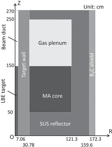
As the ADS core, the basic concept investigated in JAEA was adopted [19]. Figure 2 shows the two-dimensional R–Z geometry of the ADS. The MA core region in the ADS is composed of fuel, cladding tubes, and LBE coolant. The volume ratio of these component materials is 0.27:0.10:0.63. The k_eff of the ADS initial core was set to 0.97 by adjusting the weight ratio of ZrN and (Pu+MA)–N. The isotopic compositions of the actinides are listed in Table 1.

Table 1. Isotopic composition of actinides in the MA core region

Nuclide	(wt%)	Nuclide	(wt%)
U-234	0.01	Am-241	23.19
Np-237	34.21	Am-242m	0.04
Pu-238	0.71	Am-243	9.68
Pu-239	16.17	Cm-243	0.02
Pu-240	7.41	Cm-244	2.95
Pu-241	3.22	Cm-245	0.29
Pu-242	2.07	Cm-246	0.03

Figure 2. Two-dimensional R–Z geometry for ADS initial core. R. Katano: Estimation of sensitivity coefficient based on lasso-type penalized linear regression.

The ADS3D code was used to perform the core calculation [20]. The criterion of outer iteration for k_eff was set to 1.0⁻⁷. We used the 73 groups’ energy structure from 0.1 eV to 20 MeV, in which the fast group constant sets (UFLIB.J40 [21]) based on JENDL-4.0 were used as nuclear data library. As the input parameters, a total of 13,286 multi-group microscopic cross-sections are taken into account: there are 73 group cross-sections for seven reactions (capture, fission, average number of neutrons per fission nu-bar, n2n, inelastic scattering, elastic scattering, and average scattering cosine mu-bar) of 26 nuclides, i.e. 13,268 = $73\times 7\times 26$. The indexes of microscopic cross-section of first energy group are listed in Table 2. The index of the $G$-th group microscopic cross-section for the $n$-th row nuclide and $r$-th column reaction is defined as:

(13) $j=G+73\times \left(r-1\right)+73\times 7\times \left(n-1\right).$(13)

Table 2. Index of the microscopic cross-section of first energy group

Nuclide	Capture	Fission	nu_bar	n2n	^Inelastic scattering	Elastic scattering	mu_bar
Fe-54	1	74	147	220	293	366	439
Fe-56	512	585	658	731	804	877	950
Fe-57	1023	1096	1169	1242	1315	1388	1461
Zr-90	1534	1607	1680	1753	1826	1899	1972
Zr-91	2045	2118	2191	2264	2337	2410	2483
Zr-92	2556	2629	2702	2775	2848	2921	2994
Zr-94	3067	3140	3213	3286	3359	3432	3505
Zr-96	3578	3651	3724	3797	3870	3943	4016
Pb-204	4089	4162	4235	4308	4381	4454	4527
Pb-206	4600	4673	4746	4819	4892	4965	5038
Pb-207	5111	5184	5257	5330	5403	5476	5549
Pb-208	5622	5695	5768	5841	5914	5987	6060
Bi-209	6133	6206	6279	6352	6425	6498	6571
Np-237	6644	6717	6790	6863	6936	7009	7082
Am-241	7155	7228	7301	7374	7447	7520	7593
Am-242m	7666	7739	7812	7885	7958	8031	8104
Am-243	8177	8250	8323	8396	8469	8542	8615
Cm-243	8688	8761	8834	8907	8980	9053	9126
Cm-244	9199	9272	9345	9418	9491	9564	9637
Cm-245	9710	9783	9856	9929	10,002	10,075	10,148
Cm-246	10,221	10,294	10,367	10,440	10,513	10,586	10,659
Pu-238	10,732	10,805	10,878	10,951	11,024	11,097	11,170
Pu-239	11,243	11,316	11,389	11,462	11,535	11,608	11,681
Pu-240	11,754	11,827	11,900	11,973	12,046	12,119	12,192
Pu-241	12,265	12,338	12,411	12,484	12,557	12,630	12,703
Pu-242	12,776	12,849	12,922	12,995	13,068	13,141	13,214

By defining the index as Equation (13)(13) $j=G+73\times \left(r-1\right)+73\times 7\times \left(n-1\right).$(13) , the adjacent elements are arranged in the order of energy; thus, the non-zero values cluster within particular energy range can be considered by the smooth-lasso.

In the random sampling, the correlation among the cross-sections is not taken into account since uncertainty estimation is not the objective of the present study. Each microscopic cross-section was uniformly sampled in the range of $\pm$5%. The relative sensitivity coefficients of k_eff to the 13,268 microscopic cross-sections are estimated with 100, 200, 500, 750, 1000, 1500, 2000, and 4000 samples. We utilized the lasso, smooth-lasso, and adaptive smooth-lasso for the sensitivity coefficients estimation. Table 3 lists the user-defined tuning parameters used in this verification calculation. For lasso, we utilize ${\lambda }_1$ in Table 3 as $\lambda$ in Equation (8)(8) $p\left(\vec{g}\right)=\lambda \sum _{j=1}^N\left|g_j\right|,$(8) . We determined the values in Table 3 through preliminary calculations so that the estimated sensitivity coefficients can well reproduce represent the reference values.

Table 3. The values of tuning parameters used for sensitivity coefficients estimation

Parameter	Value
λ1	1.0e–4
λ2	0.10
c	30.0
γ	0.50

The reference values of the relative sensitivity coefficients are evaluated with the direct forward method with the central difference approximation using 5% perturbation (i.e. one non-perturbed forward calculation and $13286\times 2$ times perturbed forward calculations are additionally performed). The difference between the estimated and reference values of the sensitivity coefficients is quantified by relative difference norm and is defined as follows:

(14) $e=\frac{{||\vec{g}}_{\mathrm{e}\mathrm{s}\mathrm{t}}-{\vec{g}}_{\mathrm{r}\mathrm{e}\mathrm{f}}|{|}_2}{{||\vec{g}}_{\mathrm{r}\mathrm{e}\mathrm{f}}|{|}_2},$(14)

where, ${\vec{g}}_{est}$ and ${\vec{g}}_{ref}$ are the sensitivity coefficients obtained by three penalized linear regression and by the direct method, respectively and $||\vec{x}|{|}_2$ represents the L2 norm of a vector $\vec{x}$. When the estimated values are equal to the reference values, the relative difference norm defined by Equation (14)(14) $e=\frac{{||\vec{g}}_{\mathrm{e}\mathrm{s}\mathrm{t}}-{\vec{g}}_{\mathrm{r}\mathrm{e}\mathrm{f}}|{|}_2}{{||\vec{g}}_{\mathrm{r}\mathrm{e}\mathrm{f}}|{|}_2},$(14) is zero.

The statistical errors of the sensitivity coefficients and the difference norm of Equation (14)(14) $e=\frac{{||\vec{g}}_{\mathrm{e}\mathrm{s}\mathrm{t}}-{\vec{g}}_{\mathrm{r}\mathrm{e}\mathrm{f}}|{|}_2}{{||\vec{g}}_{\mathrm{r}\mathrm{e}\mathrm{f}}|{|}_2},$(14) with the lasso, the smooth-lasso, and the adaptive smooth-lasso are evaluated by the resampling technique, i.e. Jackknife technique [22].

3.2. Results

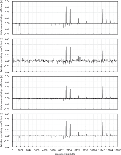
Figure 3 shows the sensitivity coefficients obtained by the direct method, lasso, smooth-lasso, and adaptive smooth-lasso with 750 samples. As shown in the result by the direct method, most of the sensitivity coefficients are zero, i.e. sparse. The result by the lasso shows that the many sensitivity coefficients are miss-predicted as non-zero values for the cross-sections whose reference value of sensitivity coefficient is zero. As can be seen from the result by the smooth-lasso and the adaptive smooth-lasso in Figure 3, some sensitivity coefficients cannot completely reproduce the reference values, although the tuning parameters are optimized. This is since the sample number of 750 is significantly smaller than the number of input parameters (i.e. 13,286 in this paper) and the information about the relation between the input parameters and the response is not enough to completely reproduce the sensitivity coefficients. However, we can observe that the smooth-lasso and the adaptive smooth-lasso can reproduce the structure of the non-zero values of the sensitivity coefficients better than the lasso.

Figure 3. Relative sensitivity coefficients of k_eff of ADS initial core with 750 samples. (Results by direct method, lasso, smooth-lasso, and adaptive smooth-lasso from top to bottom.) R. Katano: Estimation of sensitivity coefficient based on lasso-type penalized linear regression.

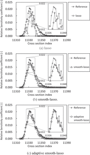
Figure 4 shows the sensitivity coefficients to the fission cross-sections of Pu-239 obtained by lasso, smooth-lasso, adaptive smooth-lasso, and the direct method with 750 samples. Figure 4(a) shows that some relative sensitivity coefficients obtained by lasso take zero or small value for the indexes where the reference values are not negligible. Figure 4(b) shows that the relative sensitivity coefficients obtained by smooth-lasso are smaller than those of reference and fail to reproduce the steep change of the sensitivity coefficients for the index. Figure 4(c) shows that the relative sensitivity coefficients obtained by adaptive smooth-lasso are emphasized to reproduce the reference values and capture the steep change tendency of the reference values compared to smooth-lasso.

Figure 4. Relative sensitivity coefficients of k_eff to the fission cross-section of Pu-239 with 750 samples. R. Katano: Estimation of sensitivity coefficient based on lasso-type penalized linear regression.

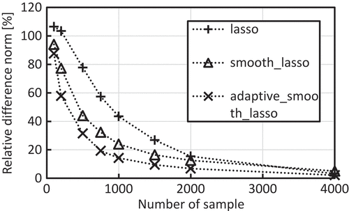
Figure 5 shows the relative difference norm for each method versus the number of samples. As shown in Figure 5, the difference norms are decreased as the number of samples increases. The relative difference norms by the lasso are the largest and those by the adaptive smooth-lasso are the smallest among the three penalized linear regressions.

Figure 5. The number of samples versus relative difference norm of relative sensitivity of k_eff of ADS initial core. R. Katano: Estimation of sensitivity coefficient based on lasso-type penalized linear regression.

Figure 6 shows the comparison of the relative sensitivity coefficients obtained by each method with 750 samples and those obtained by the direct method. In Figure 6, the horizontal and vertical axes represent the relative sensitivity coefficients of the k_eff obtained by the direct method and each method, respectively. The error bars in Figure 6 are the standard deviations estimated by the Jackknife technique. As shown in Figure 6(a), we observe the ‘cross’ plots centered at the origin in the lasso result. This result indicates that the sensitivity coefficients are miss-predicted as non-zero values for the cross-sections whose sensitivity coefficients are zero, and vice versa. This is because the lasso does not consider the structure of the non-zero elements for energy. In addition, the error bars of the lasso result are larger than those of the smooth-lasso and the adaptive smooth-lasso results. This is also because the structure of the non-zero elements is not taken into account, i.e. the indexes for non-zero sensitivity coefficients are frequently changed according to the Jackknife resample of cross-sections. In Figure 5, due to the cross plots, the error norm by the lasso is largest among the three estimation methods. In Figure 6(b, c), we cannot observe the cross plots and the error bars are smaller than those of the lasso result. These results indicate that the smooth-lasso and adaptive smooth-lasso well reproduce the structure of the non-zero elements of sensitivity coefficients compared to the lasso. As shown in Figure 6(b), most of the absolute values of sensitivity coefficients obtained by the smooth-lasso are smaller than those of reference. The sensitivity coefficients whose neighbor sensitivity coefficient is zero or small are underestimated since the smooth-lasso selects the solution whose adjacent elements take close values. Consequently, the smooth-lasso fails to accurately reproduce the steep changes of the sensitivity coefficients for the energy and underestimates the absolute values of sensitivity coefficients.

Figure 6. Comparison of relative sensitivity coefficients of k_eff of ADS initial core. The number of samples is 750. R. Katano: Estimation of sensitivity coefficient based on lasso-type penalized linear regression.

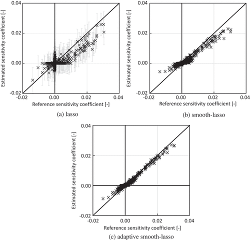
The adaptive smooth-lasso reduces the underestimation tendency compared to the smooth-lasso as shown in Figure 6(c). This is because the large absolute values of sensitivity coefficients are emphasized and the steep changes of the sensitivity coefficients are allowed by the weighted penalty term of the adaptive smooth-lasso. Because the cross plots and underestimation tendencies are mitigated, the relative difference norm by the adaptive smooth-lasso is smallest among the three penalized linear regressions as shown in Figure 5. These results indicate that the adaptive smooth-lasso proposed in this study can be a candidate for a practical estimation method of the sensitivity coefficients without adjoint calculations.

4. Conclusion

We propose the adaptive smooth-lasso as an estimation method of the sensitivity coefficients of the neutronics parameters using the random sampling. The proposed method is based on a lasso-type penalized linear regression. The proposed method utilizes the weighted penalty term aiming to reproduce the sensitivity coefficients having steep energy dependence with a small number of samples. The proposed method utilizes only forward calculations. In addition, the proposed method can reduce the calculation costs compared to the conventional random sampling method. Therefore, the proposed method can be a candidate for the practical estimation method of the sensitivity coefficients when the application of the adjoint method is difficult due to the complexity of the code system and/or the difficulty of the definition of the adjoint model for such complicated code system.

To verify the proposed method, three lasso-type penalized regressions including the proposed method were applied for the estimation of the relative sensitivity coefficients of k_eff of an ADS. A total of 13,286 cross-sections, i.e. 73-group microscopic cross-sections of 26 nuclides, are taken into account. Through the verification calculation, it is confirmed that sensitivity coefficients obtained by the proposed method can accurately reproduce those of the direct method with smaller samples compared to the lasso and smooth-lasso.

The proposed method requires four user-defined tuning parameters. In this paper, the tuning parameters were determined through preliminary calculations so that the estimation result well reproduce the reference values. However, in practical applications, these parameters should be optimized without the reference values. The optimization of the parameters would be a future task. For example, in the case of the lasso, the CV technique can be used to optimize the lasso tuning parameter using only the sample set. Thus, the CV technique may be applicable to the proposed method.

The verification in this paper was performed under simple calculation conditions and the number of the target neutronics parameters is one (k_eff). Under these conditions, the adjoint method is superior. Estimation of the sensitivity coefficients of the various neutronics parameters (e.g. beam current of the accelerator of ADS, spatial power distribution, and nuclide number density) under the complicated conditions (e.g. burnup and refueling) using the present method would be also a future task.

Disclosure statement

No potential conflict of interest was reported by the authors.

References

- Iwamoto H, Nishihara K, Sugawara T, et al. Sensitivity and uncertainty analysis for an accelerator driven system with JENDL-4.0. J Nucl Sci Technol. 2013;50:856–862.
- Takeda T, Yoshimura Y. Prediction uncertainty evaluation methods to core performance parameters in large liquid-metal fast breeder reactor. Nucl Sci Eng. 1989;103:257.
- Chiba G, Narabayashi T. Variance reduction factor of nuclear data for integral neutronics parameters. Nuclear Data Sheets. 2015;123:62–67.
- Usachev LN. Perturbation theory for the breeding ratio and for other number ratios pertaining to various reactor processes. J Nucl Energy A/B. 1964;18:571–583.
- Williams M. Development of depletion perturbation theory for coupled neutron/nuclide fields. Nucl Sci Eng. 1979;70:20–36.
- Chiba G, Pyeon CH, WFG VR, et al. Nuclear data-induced uncertainty quantification of neutronics parameters of accelerator-driven system. J Nucl Sci Technol. 2016;53:1653–1661.
- Katano R, Endo T, Yamamoto A. Estimation of sensitivity coefficients of core characteristics based on reduced-order modeling using sensitivity matrix of assembly characteristics. J Nucl Sci Thecnol. 2017;54:637–647.
- Kennedy C, Rabiti C, Abdel-Khalik H. Generalized perturbation theory free sensitivity analysis for eigenvalue problems. Nucl Technol. 2012;179:169–179.
- Wang C, Abdel-Khalik H. Exact-to-precision generalized perturbation theory for reactor design calculations. In: Proc PHYSOR 2014; 2014 Sep 28–Oct 3; Kyoto, Japan.
- Bang Y, Abdel-Khalik H. Sensitivity analysis via reduced order adjoint method. In: Proc PHYSOR 2014; 2014 Sep 28–Oct 3; Kyoto, Japan.
- Abdo M, Abdel-Khalik H. Development of multi-level reduced order modeling methodology. Trans Am Nucl Soc. 2015;112:445–448.
- Chiba G, Kawamoto Y, Tsuji M, et al. Estimation of neutronics parameter sensitivity to nuclear data in random sampling-based uncertainty quantification calculations. Ann Nucl Energy. 2015;75:395–403.
- Watanabe T, Endo T, Yamamoto A, et al. Estimation of sensitivity coefficient using random sampling and L1-norm minimization. Trans Am Nucl Soc. 2014;111:1391–1394.
- Candes E, Wakin M. An introduction to compressive sampling. IEEE Signal Process Mag. 2008;25(2):21–30.
- Tibshirani R. Regression shrinkage and selection via the lasso. J. R Statist Soc. 1996;58:267–288.
- Hawkins D, Maboudou-Tchao E. Smoothed linear modeling for smooth spectral data. Int J Spectrosc. 2013; [8 p.].
- Nozad M. Sparse ridge fusion for linear regression [ master’s thesis]. Orlando (FL): the University of Central Florida; 2013.
- Lund KV. The instability of cross-validated lasso [ master’s thesis]. Oslo (Norway). University of Oslo; 2013.
- Tsujimoto K, Sasa T, Nishihara K, et al. Neutronics design for lead-bismuth cooled accelerator-driven System for transmutation of minor actinide. J Nucl Sci Technol. 2004;41:21–36.
- Sugawara T, Nishihara K, Iwamoto H, et al. Development of three-dimensional reactor analysis code system for accelerator-driven system, ADS3D and its application with subcriticality adjustment mechanism. J Nucl Sci Technol. 2016;53:2018–2027.
- Sugino K, Jin T, Hazama T, et al. Preparation of fast reactor group constant sets UFLIB.J40 and JFS-3-J4.0 based on the JENDL-4.0 data. Ibaraki (Japan): Japan Atomic Energy Agency; 2012. JAEA-Data/Code 2011-017.
- Efron B. The jackknife, the bootstrap, and other resampling plans. Philadelphia (PA): Society for Industrial and Applied Mathematics; 1982.