Monte Carlo criticality analysis of random media under bounded fluctuation driven by normal noise

ABSTRACT

In Monte Carlo criticality analysis under material distribution uncertainty, it is necessary to evaluate the response of neutron effective multiplication factor (k_eff) to the space-dependent random fluctuation of volume fractions within a prescribed bounded range. Normal random variables, however, cannot be used in a straightforward manner since the normal distribution has infinite tails. To overcome this issue, a methodology has been developed via forward–backward-superposed reflection Brownian motion (FBSRBM). Here, the forward–backward superposition makes the variance of fluctuation spatially constant and the reflection Brownian motion confines the fluctuation driven by normal noise in a bounded range. In addition, the power spectrum of FBSRBM remains the same as that of Brownian motion. FBSRBM was implemented using Karhunen–Loève expansion (KLE) and applied to the fluctuation of volume fractions in a model of UO₂–concrete media with stainless steel. Numerical results indicate that the non-negligible and significant fluctuation of k_eff arises due to the uncertainty of media formation and just a few number of terms in KLE are enough to ensure the reliability of criticality calculation.

KEYWORDS:

• Criticality
• random media
• bounded fluctuation
• normal noise
• Brownian motion
• Karhunen–Loève expansion

1. Introduction

In many cases of engineering analysis, it is necessary to evaluate system responses to the random fluctuation of some parameter within a prescribed range with upper and lower bounds. It is known in information theory [1] that normal random variables have the largest entropy under the constraint of a fixed value of variance. Engineers are thus motivated to utilize normal noise in the response evaluation. However, the infinite tails of normal distribution have been a major hurdle to the modeling of bounded fluctuation, and this issue arises in the criticality analysis of debris as well. The present work proposes a methodology for the bounded fluctuation driven by normal noise and demonstrates numerical results for its application to the spatial fluctuation of volume fractions in a model of UO₂–concrete media with stainless steel precipitates. The methodology can be utilized as a tool for Monte Carlo (MC) criticality analysis under material distribution uncertainty in addition to the randomized Weierstrass function (RWF) developed previously [2].

The log normal transformation has been traditionally utilized for the modeling of one-sided-bounded fluctuation originated from normal noise. In the nuclear engineering disciplines, the log-normal transformation is investigated in computational radiation transport [3]. As opposed to these popularities, a different approach must be pursued for the modeling of the spatial variation in volume fractions since volume fractions are strictly bounded above and below, respectively, by 100% and 0%. The model and mechanism chosen for this pursuit are Brownian motion (BM) [4] and the equivalence in likelihood between the original and reflected BM paths [5]. Previous work based on the reflection of BM path is found in the disciplines of operations research and management science within the context of the asymptotic variance of a stationary simulation output process [6]. In the present work, multiple reflections are justified based on the strong Markov property in stochastic analysis [5] and the reflected BM path is shown to have the same power spectrum as that of the BM path characterized by the inverse-square law [7]. Other noteworthy aspect of BM is the linear growth of variance [4]. If forward and backward BM paths are independently superposed, the synthesized path has constant variance throughout the domain. Based on these approaches with reflection and superposition, it is possible to generate replicas of the path with constant variance driven by normal noise and characterized by a strictly bounded fluctuation range. The methodology developed is to be termed the forward–backward-superposed reflection Brownian motion (FBSRBM).

An ideal approach often ends up with some compromise for a feasibility reason. In the present work, the Karhunen–Loève expansion (KLE) [8,9] of stochastic processes is chosen to approximate a BM path. The reason for this choice is that the eigenvalue spectrum decomposition of BM covariance function in KLE matches very well with the inverse-square power spectrum of BM [7]. The integrated error minimality at expansion truncation is also a favorable aspect of KLE [8]. Numerical results are demonstrated for the MC criticality calculation of the UO₂–concrete media with stainless steel precipitates where the mean volume ratio of UO₂-to-concrete is set close to the optimal moderation condition [10]. Voxel mesh overlay is a mechanism for handling stainless steel precipitates.

Before concluding this section, it is worthwhile mentioning other motivation behind the development of FBSRBM. In the previous work on MC criticality analysis under material distribution uncertainty [2], the random media modeling with RWF was compared against the deterministic spatial fluctuation modeling with the strict conservation of the total volume of each constituent material. Its numerical results indicate that the largest neutron effective multiplication factor (k_eff) is obtained for a deterministic trigonometric fluctuation, although the total volume of UO₂ is not conserved in the RWF modeling. Similar comparison should be conducted for different random media modeling before making any conclusion on random media versus deterministic fluctuation. It is thus necessary to develop random modeling different from RWF. To that end, FBSRBM is chosen because of three target characteristics: (1) upper and lower fluctuation bounds, (2) constant variance, and (3) normal noise.

2. BM, reflection, and superposition

BM was originally proposed as an idealized model of the phenomenon discovered in a continual swarming motion of pollen grains in water. In the modern probability theory, BM is a nonstationary stochastic process with the stationary increments of normal distribution. Its formal definition is [4]:

Definition (BM):

(A) For $0\le x_0<x_1<x_2<\cdots <x_m$, $B_M(x_0)$, $B_M(x_1)-B_M(x_0)$, $B_M(x_2)-B_M(x_1)$,$\cdots$, $B_M(x_m)-B_M(x_{m-1})$ are independent,

(B) $\begin{array}{rl}& P_R(B_M^{\hspace{0.17em}}(x+h)-B_M^{\hspace{0.17em}}(x)\le z)=(2\pi h{)}^{-1/2}\\ & \underset{-\mathrm{\infty }}{\overset{z}{\int }}exp(-u^2/(2h))du,x\ge 0,h>0,\end{array}$

(C) $P_R(B_M(0)=0)=1$ and $B_M^{\hspace{0.17em}}(x)$ is continuous with probability 1 for $x\ge 0$,

where $B_M(x)$ stands for BM with the argument x as the explicit indication of domain variable and implies the path value evaluated at x; $P_R$ stands for probability. Three different proofs exist for the existence of BM [5].

Two aspects of BM deserve immediate attention. First, as stated in Definition (BM-A), the increments $\mathrm{\Delta }{B}_M(x,h)\equiv B_M(x+h)-B_M(x)$ are independent for all $x\ge 0$ and $h>0$ if the intervals $(x,x+h]$ do not overlap. Second, the law of normal distribution in Definition (BM-B) implies that $\mathrm{\Delta }{B}_M(x,h)=\mathrm{\Delta }Y$ and $\mathrm{\Delta }{B}_M(x,h)=-\mathrm{\Delta }Y$ are equally likely to occur. For these reasons, both $B_M(x)$ and its reflection at $B_M(x)=Y$ are paths that are equally likely to occur. This property of BM is formally based on the following theorem:

(Theorem) Define $S_Y=inf\{x>0;B_M(x)=Y\}$. Then, with $B_M^{\prime }(x)\equiv B_M(S_Y+x)-B_M(S_Y)$ for $x\ge 0$, the process $B_M^{\prime }$ is also BM; $B_M^{\prime }(x)$ follows the laws in Definitions (BM-A, B, C).

(Remark) According to stochastic analysis, S_Y belongs to two classes of random variables called optional time and stopping time. The above theorem holds for the optional time due to the strong Markov property of BM. The details can be found in the proof of 6.16 Theorem in Chapter 2 in [5].

Definition (BM) and the symmetry of normal distribution imply that the path defined by$B_M(x)$ for $x\le S_Y$ and $Y-B_M^{\prime }(x-S_Y)$ for $x>S_Y$ is also a path of BM. If this path reaches the level Y after x increases by a finite amount S, Theorem is again applied to generate the new BM path starting afresh as $B_M^{\prime \prime }(x)\equiv B_M^{\prime }(S+x)-B_M^{\prime }(S)$, $x>0$. Then, the path defined by$B_M(x)$ for $x\le S_Y$, $Y-B_M^{\prime }(x-S_Y)$ for $S_Y<x<S_Y+S$ and $Y-B_M^{\prime \prime }(x-S_Y-S)$ for $x>S_Y+S$ is also a path of BM. In this manner, whenever BM crosses the level Y, its path is reflected and the resulting path remains BM. Such a mechanism can be utilized to realize paths confined above the level Y₁ (<0) and below the level Y₂ (>0).

For demonstration, it is worthwhile to show $B_M(x)$ and its reflection path. Since the covariance of BM is [4]:

(1) $E[B_M(x_1)B_M(x_2)]=min(x_1,x_2)=\frac{1}{2}[x_1+x_2-\left|x_1-x_2\right|]$(1)

where E denotes expectation, the covariance matrix $\mathbf{C}=(C_{j,k}^{\hspace{0.17em}})$ is introduced as:

(2) $\begin{array}{rl}& C_{j,k}^{\hspace{0.17em}}\equiv E[B_M^{\hspace{0.17em}}(x_j)B_M^{\hspace{0.17em}}(x_k)]=min(x_j,x_k),\\ & x_j=\frac{j}{n},x_k=\frac{k}{n},j,k=1,\dots ,n\end{array}$(2)

The symmetry and positive definiteness of covariance matrices allow one to express the matrix C as the product of a lower triangular matrix L and its transpose L^T:

(3) $\mathbf{C}=(C_{i,j})=\mathbf{L}\mathbf{L}{ }^{\mathrm{T}}.$(3)

Let $\mathbf{V}\equiv (V_1,V_2,\dots ,V_n)$ be a vector of independent random variables under the standard normal distribution satisfying E[V_j] = 0, E[(V_j)²] = 1, and E[V_jV_k] = 0 for j ≠ k where the subscripts of V_j and V_k corresponds to x_j and x_k. The covariance matrix of LV becomes equal to $\mathbf{C}=\mathbf{L}{\mathbf{L}}^{\mathrm{T}}$. A replica of BM path, denoted as ${\hat{B}}_M(x)$, is generated as:

(4) $\left({\hat{B}}_M(x_1),{\hat{B}}_M(x_2),\dots ,{\hat{B}}_M(x_n)\right)=(\mathbf{L}\mathbf{V}{)}^T.$(4)

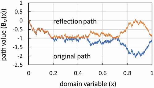
Note that once ${\hat{B}}_M(x)$ is obtained for $0\le x\le 1$, ${\hat{B}}_M(x)$ can also be obtained for $0\le x\le X$ using the equivalence in distribution between $B_M(Xx)$ and $X^{1/2}{B}_M(x)$ [4]. Only the number of domain values n matters. Figure 1 shows a path ${\hat{B}}_M(x)$ generated by Equation (4)(4) $\left({\hat{B}}_M(x_1),{\hat{B}}_M(x_2),\dots ,{\hat{B}}_M(x_n)\right)=(\mathbf{L}\mathbf{V}{)}^T.$(4) with n = 20,000 and its reflection path at the level $Y=-1$. As argued earlier, both paths are equally likely to occur. The power spectrum of ${\hat{B}}_M(x)$ can be computed as [7]:

(5) $\mathrm{\Phi }({\hat{B}}_M;f)=\hspace{0.17em}\left|\frac{1}{n}{\sum }_{j=1}^n{\hat{B}}_M\left(\frac{j}{n}\right)\right.{\left.exp\left(-i2\pi f\frac{j}{n}\right)\right|}^2$(5)

Figure 1. Brownian motion path and its refection path generated via 20,000-by-20,000 covariance matrix (n = 20,000).

where f is the frequency domain variable and i in the argument of exponential is the imaginary unit ($i^2=-1$). For BM, power spectrum is known to follow the inverse-square law [11,12]:

(6) $\mathrm{\Phi }({\hat{B}}_M;f)\propto \frac{1}{f^2}.$(6)

Therefore, it is worthwhile checking if both paths in Figure 1 follow Equation (6)(6) $\mathrm{\Phi }({\hat{B}}_M;f)\propto \frac{1}{f^2}.$(6) . Figure 2 shows the power spectrum computed by Equation (5)(5) $\mathrm{\Phi }({\hat{B}}_M;f)=\hspace{0.17em}\left|\frac{1}{n}{\sum }_{j=1}^n{\hat{B}}_M\left(\frac{j}{n}\right)\right.{\left.exp\left(-i2\pi f\frac{j}{n}\right)\right|}^2$(5) for the original and reflection path in Figure 1. It is seen that both paths almost follow the law in Equation (6)(6) $\mathrm{\Phi }({\hat{B}}_M;f)\propto \frac{1}{f^2}.$(6) . Figure 3 shows slope estimates of $\mathrm{\Phi }({\hat{B}}_M;f)$ for 200 replicas of BM independently generated by Equation (4)(4) $\left({\hat{B}}_M(x_1),{\hat{B}}_M(x_2),\dots ,{\hat{B}}_M(x_n)\right)=(\mathbf{L}\mathbf{V}{)}^T.$(4) . Figure 3 also presents the p-value of these estimates by the normality test of Shapiro–Wilk [13] extended by Royston [14]. It is seen that the deviation of ±0.28 from −2.01 is likely to occur with 95% significance. Taking this into account, one is led to conclude that both two power spectra in Figure 2 follow the inverse-square law in Equation (6)(6) $\mathrm{\Phi }({\hat{B}}_M;f)\propto \frac{1}{f^2}.$(6) and thus the reflection path in Figure 1 is indeed a realization of BM path.

Figure 2. Power spectra of Brownian motion path and its refection path generated via 20,000-by-20,000 covariance matrix (n = 20,000).

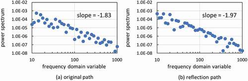
Figure 3. Slope estimate of power spectrum for Brownian motion path in [0,1] generated via 20,000-by-20,000 covariance matrix.

The development thus far demonstrate that the reflections at $Y=\pm \epsilon$ can generate BM paths confined in $[-\epsilon ,\epsilon ]$. On the other hand, it is also essential to have the capability of producing a fluctuation whose variance is constant over the domain. In order to realize a normal fluctuation with constant variance, one can utilize the linear growth property of variance implied in Equation (1)(1) $E[B_M(x_1)B_M(x_2)]=min(x_1,x_2)=\frac{1}{2}[x_1+x_2-\left|x_1-x_2\right|]$(1) with $x_1=x_2$. Let independent forward and backward BMs be denoted by $B_M^F(x)$ and $B_M^B(X-x)$, respectively, where the capital letter X corresponds to the domain size. Then, the variance of their superposition is easily shown to be constant using their independence and zero mean properties and Equation (1)(1) $E[B_M(x_1)B_M(x_2)]=min(x_1,x_2)=\frac{1}{2}[x_1+x_2-\left|x_1-x_2\right|]$(1) :

(7) $E[(B_M^F(x)+B_M^B(X-x){)}^2]=x+X-x=X.$(7)

Similarly, the covariance of this superposed process is obtained as:

(8) $\begin{array}{c}E[(B_M^F(x_1)+B_M^B(X-x_1))(B_M^F(x_2)+B_M^B(X-x_2))]\\ =E[B_M^F(x_1)B_M^F(x_2)]+E[B_M^B(X-x_1)B_M^B(X-x_2)]\\ =X-\left|x_1-x_2\right|.\end{array}$(8)

It is clear from Equations (1)(1) $E[B_M(x_1)B_M(x_2)]=min(x_1,x_2)=\frac{1}{2}[x_1+x_2-\left|x_1-x_2\right|]$(1) and (8(8) $\begin{array}{c}E[(B_M^F(x_1)+B_M^B(X-x_1))(B_M^F(x_2)+B_M^B(X-x_2))]\\ =E[B_M^F(x_1)B_M^F(x_2)]+E[B_M^B(X-x_1)B_M^B(X-x_2)]\\ =X-\left|x_1-x_2\right|.\end{array}$(8) ) that the covariance of $B_M^F(x)+B_M^B(X-x)$ is not equal to that of$B_M(x)$. This disagreement about covariance may make the power spectrum of $B_M^F(x)+B_M^B(X-x)$ deviate from the inverse-square law in Equation (6)(6) $\mathrm{\Phi }({\hat{B}}_M;f)\propto \frac{1}{f^2}.$(6) . 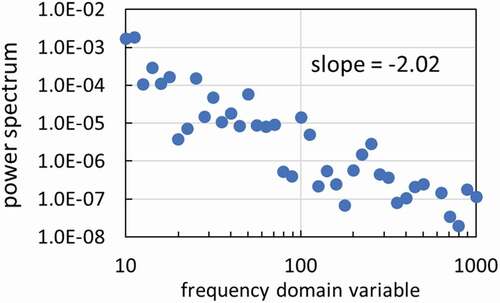Figure 4 shows power spectrum for a replica of $B_M^F(x)+B_M^B(1-x)$, i.e. $\mathrm{\Phi }({\hat{B}}_M^F(x)+{\hat{B}}_M^B(1-x);f)$. Although f-Φ plots in Figure 4 appear to be more scattered than those of Figure 2, the slope of$\mathrm{\Phi }({\hat{B}}_M^F(x)+{\hat{B}}_M^B(1-x);f)$ still follows the inverse-square law in Equation (6)(6) $\mathrm{\Phi }({\hat{B}}_M;f)\propto \frac{1}{f^2}.$(6) . This can be qualitatively explained as follows. The power spectrum of ${\hat{B}}_M^F(x)+{\hat{B}}_M^B(1-x)$ is computed as:

(9) $\begin{array}{l}|\frac{1}{n}{\displaystyle {\sum }_{j=1}^n({\widehat{B}}_M^F(\frac{j}{n})+{\widehat{B}}_M^B(1-\frac{j}{n}))\mathrm{e}{xp(-i2\pi f\frac{j}{n})|}^2}\\ =|\frac{1}{n}{\displaystyle {\sum }_{j=1}^n{\widehat{B}}_M^F(\frac{j}{n})\exp \left(-i2\pi f\frac{j}{n}\right)}\\ +\frac{1}{n}{\displaystyle {\sum }_{j=0}^{n-1}{{\widehat{B}}_M^B\left(1-\frac{j}{n}\right)\exp (-i2\pi f\frac{j}{n})-\frac{{\widehat{B}}_M^B(1)}{n}|}^2}\\ =|\frac{1}{n}{\displaystyle {\sum }_{j=1}^n{{\widehat{B}}_M^F(\frac{j}{n})\exp (-i2\pi f\frac{j}{n})|}^2}\\ +|\frac{1}{n}{\displaystyle {\sum }_{j=0}^{n-1}{{\widehat{B}}_M^B(1-\frac{j}{n})\exp (-i2\pi f\frac{j}{n})|}^2}\\ +2\text{Re}\frac{1}{n}\sum j=1n{\widehat{B}}_M^F(\frac{j}{n})\\ \exp \left](-i2\pi f\frac{j}{n})\frac{1}{n}\sum j=0n-1{\widehat{B}}_M^B(1-\frac{j}{n})\exp (i2\pi f\frac{j}{n})\right]\\ +O(1/n)\end{array}$(9)

Figure 4. Power spectrum of forward and backward superposed path from two independent replicas of Brownian motion.

where ${\hat{B}}_M^B(0)=0$ is used at the first equality and the fourth term after the second equality is the big-oh notation about the order of magnitude; $O(x)/x$ stays finite as $x\to 0$. Since ${\hat{B}}_M^B$ is real and $\left|exp(i2\pi f)\right|=1$, the second term after the second equality can be manipulated as:

(10) $\left|{\displaystyle {\sum }_{j=0}^{n-1}{\widehat{B}}_M^B\left(1-\frac{j}{n}\right)\exp \left(-i2\pi f\frac{j}{n}\right)}\right|=\left|{\displaystyle {\sum }_{j=0}^{n-1}{\widehat{B}}_M^B\left(\frac{n-j}{n}\right)\exp \left(-i2\pi f\frac{n-j}{n}\right)}\right|.$(10)

By Equations (6)(6) $\mathrm{\Phi }({\hat{B}}_M;f)\propto \frac{1}{f^2}.$(6) and (10(10) $\left|{\displaystyle {\sum }_{j=0}^{n-1}{\widehat{B}}_M^B\left(1-\frac{j}{n}\right)\exp \left(-i2\pi f\frac{j}{n}\right)}\right|=\left|{\displaystyle {\sum }_{j=0}^{n-1}{\widehat{B}}_M^B\left(\frac{n-j}{n}\right)\exp \left(-i2\pi f\frac{n-j}{n}\right)}\right|.$(10) ), the first two terms after the second equality of Equation (9)(9) $\begin{array}{l}|\frac{1}{n}{\displaystyle {\sum }_{j=1}^n({\widehat{B}}_M^F(\frac{j}{n})+{\widehat{B}}_M^B(1-\frac{j}{n}))\mathrm{e}{xp(-i2\pi f\frac{j}{n})|}^2}\\ =|\frac{1}{n}{\displaystyle {\sum }_{j=1}^n{\widehat{B}}_M^F(\frac{j}{n})\exp \left(-i2\pi f\frac{j}{n}\right)}\\ +\frac{1}{n}{\displaystyle {\sum }_{j=0}^{n-1}{{\widehat{B}}_M^B\left(1-\frac{j}{n}\right)\exp (-i2\pi f\frac{j}{n})-\frac{{\widehat{B}}_M^B(1)}{n}|}^2}\\ =|\frac{1}{n}{\displaystyle {\sum }_{j=1}^n{{\widehat{B}}_M^F(\frac{j}{n})\exp (-i2\pi f\frac{j}{n})|}^2}\\ +|\frac{1}{n}{\displaystyle {\sum }_{j=0}^{n-1}{{\widehat{B}}_M^B(1-\frac{j}{n})\exp (-i2\pi f\frac{j}{n})|}^2}\\ +2\text{Re}\frac{1}{n}\sum j=1n{\widehat{B}}_M^F(\frac{j}{n})\\ \exp \left](-i2\pi f\frac{j}{n})\frac{1}{n}\sum j=0n-1{\widehat{B}}_M^B(1-\frac{j}{n})\exp (i2\pi f\frac{j}{n})\right]\\ +O(1/n)\end{array}$(9) follow the inverse-square law with respect to f. Similarly, the absolute values of:

(11) $\frac{1}{n}{\displaystyle {\sum }_{j=1}^n{\widehat{B}}_M^F\left(\frac{j}{n}\right)\exp \left(-i2\pi f\frac{j}{n}\right)}$(11)

and

(12) $\frac{1}{n}{\displaystyle {\sum }_{j=0}^{n-1}{\widehat{B}}_M^B\left(1-\frac{j}{n}\right)\exp \left(i2\pi f\frac{j}{n}\right)}=\frac{\exp (i2\pi f)}{n}{\displaystyle {\sum }_{j=0}^{n-1}{\widehat{B}}_M^B\left(\frac{n-j}{n}\right)\exp \left(-i2\pi f\frac{n-j}{n}\right)}$(12)

are both proportional to $1/f$ by Equation (6)(6) $\mathrm{\Phi }({\hat{B}}_M;f)\propto \frac{1}{f^2}.$(6) . The third term after the second equality of Equation (9)(9) $\begin{array}{l}|\frac{1}{n}{\displaystyle {\sum }_{j=1}^n({\widehat{B}}_M^F(\frac{j}{n})+{\widehat{B}}_M^B(1-\frac{j}{n}))\mathrm{e}{xp(-i2\pi f\frac{j}{n})|}^2}\\ =|\frac{1}{n}{\displaystyle {\sum }_{j=1}^n{\widehat{B}}_M^F(\frac{j}{n})\exp \left(-i2\pi f\frac{j}{n}\right)}\\ +\frac{1}{n}{\displaystyle {\sum }_{j=0}^{n-1}{{\widehat{B}}_M^B\left(1-\frac{j}{n}\right)\exp (-i2\pi f\frac{j}{n})-\frac{{\widehat{B}}_M^B(1)}{n}|}^2}\\ =|\frac{1}{n}{\displaystyle {\sum }_{j=1}^n{{\widehat{B}}_M^F(\frac{j}{n})\exp (-i2\pi f\frac{j}{n})|}^2}\\ +|\frac{1}{n}{\displaystyle {\sum }_{j=0}^{n-1}{{\widehat{B}}_M^B(1-\frac{j}{n})\exp (-i2\pi f\frac{j}{n})|}^2}\\ +2\text{Re}\frac{1}{n}\sum j=1n{\widehat{B}}_M^F(\frac{j}{n})\\ \exp \left](-i2\pi f\frac{j}{n})\frac{1}{n}\sum j=0n-1{\widehat{B}}_M^B(1-\frac{j}{n})\exp (i2\pi f\frac{j}{n})\right]\\ +O(1/n)\end{array}$(9) is thus proportional to $1/f^2$ and accompanied by an f-dependent phase shift. Therefore, taking Equation (8)(8) $\begin{array}{c}E[(B_M^F(x_1)+B_M^B(X-x_1))(B_M^F(x_2)+B_M^B(X-x_2))]\\ =E[B_M^F(x_1)B_M^F(x_2)]+E[B_M^B(X-x_1)B_M^B(X-x_2)]\\ =X-\left|x_1-x_2\right|.\end{array}$(8) into account, $B_M^F(x)+B_M^B(1-x)$ can be viewed as a stationary approximation to the process of the $1/f^2$ power spectrum with a phase-shift-related fluctuation. This characterization of $B_M^F(x)+B_M^B(1-x)$ agrees with nearly the same f-Φ plots in Figures 2 and 4.

Based on these developments, one can generate a superposed-BM-path driven by normal noises and confined in $[-\epsilon ,\epsilon ]$. Let the initial value be $\hat{F}(x)={\hat{B}}_M^F(x)+{\hat{B}}_M^B(1-x)$ and evaluate the final value of $\hat{F}(x)$ by the algorithm below:

Algorithm (reflection):

$\hat{F}(x)={\hat{B}}_M^F(x)+{\hat{B}}_M^B(1-x);$

while ($\left|\hat{F}(x)\right|>\epsilon$) {

if ($\hat{F}(x)>\epsilon )$ {$\hat{F}(x)=2\epsilon -\hat{F}(x);$}

else if ($\hat{F}(x)<-\epsilon$) {$\hat{F}(x)=-2\epsilon -\hat{F}(x);$}

}

Since $2(\pm \epsilon )-({\hat{B}}_M^F(x)+{\hat{B}}_M^B(1-x))=2(\pm \epsilon /2)$$-{\hat{B}}_M^F(x)+2(\pm \epsilon /2)-{\hat{B}}_M^B(1-x)$, the successive reflections of ${\hat{B}}_M^F(x)$ and ${\hat{B}}_M^B(1-x)$ at $Y=\pm \epsilon /2$ occur in the above computation until $\left|\hat{F}(x)\right|\le \epsilon$ is satisfied. This path realization method is to be termed the FBSRBM. Note that FBSRBM is an approximate 1/f²-spectrum fluctuation of constant variance. This approximation has been shown directly from the defining formula of power spectrum while the RWF in previous work [2] is connected indirectly to a family of 1/f^2α+1 power spectrum ($0<\alpha <1$) via moment properties and fractal dimension.

3. KLE of BM

The storage space for a replica of BM path computed by Equation (4)(4) $\left({\hat{B}}_M(x_1),{\hat{B}}_M(x_2),\dots ,{\hat{B}}_M(x_n)\right)=(\mathbf{L}\mathbf{V}{)}^T.$(4) can be prohibitively large for real applications. To overcome this efficiency issue, candidate techniques to look at can be searched among well-defined series expansion methods of stochastic processes. One of such methods is KLE utilized for uncertainty quantification [8,9]. Suppose that $C_G(x_1,x_2)$ is the covariance function of a stochastic process $G(x)$ with zero mean,

(13) $E[G(x)]=0.$(13)

The eigenvalue problem of C_G is:

(14) $\underset{x_{min}}{\overset{x_{max}}{\int }}{C}_G(x_1,x_2)g_m(x_2)d{x}_2=e_m{g}_m(x_1),$(14)

where the eigenvalues e are non-negative and ordered as $e_1\ge e_2\ge \cdots$ and the eigenfunctions g are an orthonormal set of functions. The KLE of $G(x)$ is then:

(15) $G(x)={\displaystyle {\sum }_{m=1}^{\infty }\sqrt{e_m}{g}_m(x){\xi }_m,}$(15)

where ${\xi }_m$ are independent random variables with zero mean and unit variance. KLE was introduced in the nuclear engineering disciplines by Williams [15] and has been actively investigated for non-normal uncertainties [16]. The application of KLE to finite dimensional sample data can be viewed as the principal component analysis [9].

For BM, the substitution of Equation (1)(1) $E[B_M(x_1)B_M(x_2)]=min(x_1,x_2)=\frac{1}{2}[x_1+x_2-\left|x_1-x_2\right|]$(1) in $C_G(x_1,x_2)$ in Equation (14)(14) $\underset{x_{min}}{\overset{x_{max}}{\int }}{C}_G(x_1,x_2)g_m(x_2)d{x}_2=e_m{g}_m(x_1),$(14) yields the eigenvalue problem:

(16) $\underset{0}{\overset{1}{\int }}min(t,u)g_m(t)dt=e_m{g}_m(u).$(16)

Equation (16)(16) $\underset{0}{\overset{1}{\int }}min(t,u)g_m(t)dt=e_m{g}_m(u).$(16) can be rewritten as:

(17) $\underset{0}{\overset{u}{\int }}t{g}_m(t)dt+u\underset{u}{\overset{1}{\int }}{g}_m(t)dt=e_m{g}_m(u).$(17)

Differentiate with respect to u:

(18) $\underset{u}{\overset{1}{\int }}{g}_m(t)dt=e_m{g}_m^{\prime }(u).$(18)

Differentiate once more:

(19) $g_m^{\prime \prime }(u)=-\frac{1}{e_m}{g}_m(u).$(19)

The general solution of Equation (19)(19) $g_m^{\prime \prime }(u)=-\frac{1}{e_m}{g}_m(u).$(19) is:

(20) $g_m(u)=A_m^{S}sin\left(\frac{u}{\sqrt{e_m}}\right)+A_m^{C}cos\left(\frac{u}{\sqrt{e_m}}\right).$(20)

Since $g_m(0)=0$ by Equation (16)(16) $\underset{0}{\overset{1}{\int }}min(t,u)g_m(t)dt=e_m{g}_m(u).$(16) , $A_m^C=0$. Equation (18)(18) $\underset{u}{\overset{1}{\int }}{g}_m(t)dt=e_m{g}_m^{\prime }(u).$(18) also implies $g_m^{\prime }(1)=0$, which leads to:

(21) $e_m=1/(\pi (m-0.5){)}^2.$(21)

Equation (20)(20) $g_m(u)=A_m^{S}sin\left(\frac{u}{\sqrt{e_m}}\right)+A_m^{C}cos\left(\frac{u}{\sqrt{e_m}}\right).$(20) becomes:

(22) $g_m(u)=A_m^{S}sin(\pi (m-0.5)u).$(22)

and the normalization condition $\underset{0}{\overset{1}{\int }}[g_m(u){]}^{2}du=1$ yields:

(23) $A_m^S=\sqrt{2}.$(23)

In Equations (21)(21) $e_m=1/(\pi (m-0.5){)}^2.$(21) and (22(22) $g_m(u)=A_m^{S}sin(\pi (m-0.5)u).$(22) ), the eigenfunctions are trigonometric and the eigenvalue spectrum is of inverse-square nature, which matches very well with the inverse-square power spectrum displayed in Equation (6)(6) $\mathrm{\Phi }({\hat{B}}_M;f)\propto \frac{1}{f^2}.$(6) .

It is known that (1) the finite dimensional distribution of $B_M(x_0)$, $B_M(x_1)$,$\cdots$, $B_M(x_k)$ is jointly normal [5] and (2) if the finite dimensional distribution of $G(x_0)=B_M(x_0)$, $G(x_1)=B_M(x_1)$,$\cdots$, $G(x_k)=B_M(x_k)$ is normal, $\xi$ in Equation (15)(15) $G(x)={\displaystyle {\sum }_{m=1}^{\infty }\sqrt{e_m}{g}_m(x){\xi }_m,}$(15) are normal random variables [17]. Equations (15)(15) $G(x)={\displaystyle {\sum }_{m=1}^{\infty }\sqrt{e_m}{g}_m(x){\xi }_m,}$(15) and (21(21) $e_m=1/(\pi (m-0.5){)}^2.$(21) )–(23(23) $A_m^S=\sqrt{2}.$(23) ) then yield:

(24) $B_M(x)=\sqrt{2}{\displaystyle {\sum }_{m=1}^{\infty }{\xi }_m\frac{\sin ((m-0.5)\pi x)}{(m-0.5)\pi },0\le x\le 1,}$(24)

where $\xi$ are independent normal random variables with zero mean and unit variance. It is worth mentioning that if the half-integer m–0.5 is replaced by the integer m, Equation (24)(24) $B_M(x)=\sqrt{2}{\displaystyle {\sum }_{m=1}^{\infty }{\xi }_m\frac{\sin ((m-0.5)\pi x)}{(m-0.5)\pi },0\le x\le 1,}$(24) becomes the KLE of Brownian bridge [7].

It is important to check if $E[(B(1){)}^2]=1$ is satisfied as required by Definitions (BM-B,C). According to Euler [18],

(25) $\frac{1}{1^2}+\frac{1}{2^2}+\frac{1}{3^2}+\cdots \cdots =\frac{{\pi }^2}{6}$(25)

which implies

(26) $\frac{1}{2^2}+\frac{1}{4^2}+\frac{1}{6^2}+\cdots =\frac{1}{2^2}\left(\frac{1}{1^2}+\frac{1}{2^2}+\frac{1}{3^2}+\cdots \right)=\frac{{\pi }^2}{24}.$(26)

Taking into account the independence, zero mean and unit variance of $\xi$, Equations (24)(24) $B_M(x)=\sqrt{2}{\displaystyle {\sum }_{m=1}^{\infty }{\xi }_m\frac{\sin ((m-0.5)\pi x)}{(m-0.5)\pi },0\le x\le 1,}$(24) –(26(26) $\frac{1}{2^2}+\frac{1}{4^2}+\frac{1}{6^2}+\cdots =\frac{1}{2^2}\left(\frac{1}{1^2}+\frac{1}{2^2}+\frac{1}{3^2}+\cdots \right)=\frac{{\pi }^2}{24}.$(26) ) yield:

(27) $E[(B_M(1){)}^2]=\frac{8}{{\pi }^2}\left(\frac{1}{1^2}+\frac{1}{3^2}+\frac{1}{5^2}+\cdots \right)=\frac{8}{{\pi }^2}\left(\frac{{\pi }^2}{6}-\frac{{\pi }^2}{24}\right)=1$(27)

as required.

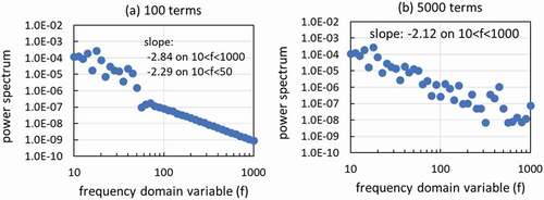
BM paths approximated by KLE are shown in Figure 5 for various numbers of expansion terms. It is clearly seen that the overall trend of BM path is already realized for 20–100 expansion terms. Figure 6 shows the slope of power spectrum for six replicas of the KLE-approximated BM path for various numbers of expansion terms. The slope estimates appear to converge within the two sigma uncertainty range in Figure 3 for numbers of expansion terms larger than or equal to 2000. Lower slope estimates for smaller numbers of expansion terms indicate that zig-zag paths due to high-frequency components will not be realized for the KLE-approximated BM paths with smaller number of expansion terms. Figure 7 shows the power spectrum of a replica of the KLE-approximated BM path for 100 and 5000 expansion terms. The power spectrum for 5000 expansion terms exhibits a nice 1/f² shape as displayed in Figure 2. This is consistent with the convergent behavior in Figure 6. On the other hand, the power spectrum for 100 expansion terms in Figure 7 exhibits steeper slope than 1/f² and appears to indicate the lack of stochasticity nature to be observed for data in high frequencies. However, for a lower frequency domain of 10 < f < 50, the power spectrum for 100 terms shows a 1/f² shape within the tolerance determined by the fluctuations in Figure 3. Therefore, in Section 4, numerical results concerning replicas of FBSRBM will be displayed for the KLE-approximated ${\hat{B}}_M^F$ and ${\hat{B}}_M^B$ from 100 expansion terms.

Figure 5. Brownian motion path constructed by Karhunen–Loève expansion with various numbers of expansion terms.

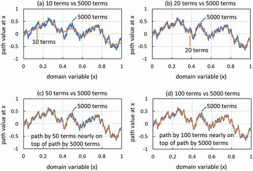
Figure 6. Slope of power spectrum evaluated on frequency domain variables in [10, 1000] for Brownian motion paths constructed by Karhunen–Loève expansions with various numbers of terms.

Figure 7. Power spectrum of Brownian motion path constructed by Karhunen–Loève expansion for replica 1 in Figure 6.

BM can be expanded in many ways as found in mathematics literatures: wavelet approach [19], an orthonormal basis expansion constructed from trigonometric and Bessel functions [20], and a basis expansion based on the orthonormality in Cameron-Martin subspace in stochastic analysis [21]. Each of these expansions is a well-established approach with a firm foundation. However, in this work, KLE has been chosen in terms of the minimality of integrated mean square error as explained below. Let the expansion of G and its residual at N-th term be:

(28) $G(x)={\displaystyle {\sum }_{j=1}^{\infty }{a}_j{g}_j(x),}$(28)

(29) $R_N(x)={\displaystyle {\sum }_{j=N+1}^{\infty }{a}_j{g}_j(x).}$(29)

The orthonormality of $\left\{g_j\right\}$ yields:

(30) $\underset{x_{min}}{\overset{x_{max}}{\int }}{g}_l(x)g_m(x)dx={\delta }_{lm},$(30)

(31) $a_j=\underset{x_{min}}{\overset{x_{max}}{\int }}G(x)g_j(x)dx,$(31)

where ${\delta }_{lm}$ is the Kronecker delta. For simplicity, the symbol denoting stochasticity such as $\omega$ in probability theory and ^ for a realization is dropped from $a_j$ and G . Also note that:

(32) $E[a_j]=0$(32)

(33) $C_G(x_1,x_2)=E[G(x_1)G(x_2)].$(33)

since G(x) was assumed to be zero mean in Equation (13)(13) $E[G(x)]=0.$(13) . The mean square error due to truncation is evaluated as the variance of the residual,

(34) $\begin{array}{rl}& E[(R_N{)}^2]=E[({\sum }_{j=N+1}^{\mathrm{\infty }}{a}_j{g}_j(x))({\sum }_{k=N+1}^{\mathrm{\infty }}{a}_k{g}_k(x))]\\ & ={\sum }_{j=N+1}^{\mathrm{\infty }}{\sum }_{k=N+1}^{\mathrm{\infty }}E[{\int }_{x_{min}}^{x_{max}}{\int }_{x_{min}}^{x_{max}}G(x_1)G(x_2)g_j(x_1)\\ & g_k(x_2)d{x}_{1}d{x}_2]g_j(x)g_k(x)={\sum }_{j=N+1}^{\mathrm{\infty }}{\sum }_{k=N+1}^{\mathrm{\infty }}{\int }_{x_{min}}^{x_{max}}{\int }_{x_{min}}^{x_{max}}\hspace{0.17em}\\ & C_G(x_1,x_2)g_j(x_1)g_k(x_2)d{x}_{1}d{x}_2{g}_j(x)g_k(x)\end{array}$(34)

where Equations (31)(31) $a_j=\underset{x_{min}}{\overset{x_{max}}{\int }}G(x)g_j(x)dx,$(31) and (33(33) $C_G(x_1,x_2)=E[G(x_1)G(x_2)].$(33) ) are used at the second and third equalities, respectively. The integration of Equation (34)(34) $\begin{array}{rl}& E[(R_N{)}^2]=E[({\sum }_{j=N+1}^{\mathrm{\infty }}{a}_j{g}_j(x))({\sum }_{k=N+1}^{\mathrm{\infty }}{a}_k{g}_k(x))]\\ & ={\sum }_{j=N+1}^{\mathrm{\infty }}{\sum }_{k=N+1}^{\mathrm{\infty }}E[{\int }_{x_{min}}^{x_{max}}{\int }_{x_{min}}^{x_{max}}G(x_1)G(x_2)g_j(x_1)\\ & g_k(x_2)d{x}_{1}d{x}_2]g_j(x)g_k(x)={\sum }_{j=N+1}^{\mathrm{\infty }}{\sum }_{k=N+1}^{\mathrm{\infty }}{\int }_{x_{min}}^{x_{max}}{\int }_{x_{min}}^{x_{max}}\hspace{0.17em}\\ & C_G(x_1,x_2)g_j(x_1)g_k(x_2)d{x}_{1}d{x}_2{g}_j(x)g_k(x)\end{array}$(34) from $x=x_{min}$ to $x=x_{max}$ and the orthonormality in Equation (30)(30) $\underset{x_{min}}{\overset{x_{max}}{\int }}{g}_l(x)g_m(x)dx={\delta }_{lm},$(30) give the integrated mean square error,

(35) $\begin{array}{l}IMS{E}_N=\underset{x_{\min }}{\overset{x_{\max }}{{\displaystyle \int }}}E[{(R_N)}^2]dx={\displaystyle \sum }_{j=N+1}^{\infty }\underset{x_{\min }}{\overset{x_{\max }}{{\displaystyle \int }}}\underset{x_{\min }}{\overset{x_{\max }}{{\displaystyle \int }}}\hfill \\ C_G(x_1,x_2)g_j(x_1)g_j(x_2)d{x}_{1}d{x}_2.\hfill \end{array}$(35)

Introduce the Lagrangian multipliers ${\lambda }_j$ for the minimization of $IMS{E}_N$ with the constraint of the normalization condition in Equation (30)(30) $\underset{x_{min}}{\overset{x_{max}}{\int }}{g}_l(x)g_m(x)dx={\delta }_{lm},$(30) :

(36) $\begin{array}{rl}& LA{G}_N={\sum }_{j=N+1}^{\mathrm{\infty }}\left[{\int }_{x_{min}}^{x_{max}}\hspace{0.17em}\right.\\ & {\int }_{x_{min}}^{x_{max}}{C}_G(x_1,x_2)g_j(x_1)g_j(x_2)d{x}_{1}d{x}_2\\ & -{\lambda }_j\left.({\int }_{x_{min}}^{x_{max}}{(g_j(x))}^{2}dx-1)\right].\end{array}$(36)

Pick some integer k larger than N and compute the variation of LAG_N due to the change of $g_k(x)$ to $g_k(x)+\eta h(x)$:

(37) $\begin{array}{rl}& LA{G}_N[g_k+\eta h]-LA{G}_N[g_k]\\ & =\eta \left[2{\int }_{x_{min}}^{x_{max}}\left({\int }_{x_{min}}^{x_{max}}{C}_G(x_1,x_2)g_k(x_2)d{x}_2-{\lambda }_k{g}_k(x_1)\right)h(x_1)d{x}_1\right]\\ & +{\eta }^2\left[{\int }_{x_{min}}^{x_{max}}{\int }_{x_{min}}^{x_{max}}h(x_1)C_G(x_1,x_2)h(x_2)d{x}_{2}d{x}_1\right.-{\lambda }_k{\int }_{x_{min}}^{x_{max}}{(h(x))}^{2}dx\end{array}$(37)

where the symmetry of the covariance function $C_G(x_1,x_2)$ is used. The condition of stationarity requires that the coefficient of η is zero for any h, which leads to:

(38) $\underset{x_{min}}{\overset{x_{max}}{\int }}{C}_G(x_1,x_2)g_k(x_2)d{x}_2={\lambda }_k{g}_k(x_1).$(38)

This is the same equation as Equation (14)(14) $\underset{x_{min}}{\overset{x_{max}}{\int }}{C}_G(x_1,x_2)g_m(x_2)d{x}_2=e_m{g}_m(x_1),$(14) [8]. In order to show the minimality of $IMS{E}_N$, one must argue if the coefficient of ${\eta }^2$ is positive for the solutions of Equation (38)(38) $\underset{x_{min}}{\overset{x_{max}}{\int }}{C}_G(x_1,x_2)g_k(x_2)d{x}_2={\lambda }_k{g}_k(x_1).$(38) . To this end, introducing the L2-norm of h as:

(39) ${∥h∥}_2={\left({\int }_{x_{min}}^{x_{max}}{(h(x))}^{2}dx\right)}^{1/2},$(39)

Equation (37)(37) $\begin{array}{rl}& LA{G}_N[g_k+\eta h]-LA{G}_N[g_k]\\ & =\eta \left[2{\int }_{x_{min}}^{x_{max}}\left({\int }_{x_{min}}^{x_{max}}{C}_G(x_1,x_2)g_k(x_2)d{x}_2-{\lambda }_k{g}_k(x_1)\right)h(x_1)d{x}_1\right]\\ & +{\eta }^2\left[{\int }_{x_{min}}^{x_{max}}{\int }_{x_{min}}^{x_{max}}h(x_1)C_G(x_1,x_2)h(x_2)d{x}_{2}d{x}_1\right.-{\lambda }_k{\int }_{x_{min}}^{x_{max}}{(h(x))}^{2}dx\end{array}$(37) is rewritten as, under Equation (38)(38) $\underset{x_{min}}{\overset{x_{max}}{\int }}{C}_G(x_1,x_2)g_k(x_2)d{x}_2={\lambda }_k{g}_k(x_1).$(38) ($e_k={\lambda }_k$ in Equation (14)(14) $\underset{x_{min}}{\overset{x_{max}}{\int }}{C}_G(x_1,x_2)g_m(x_2)d{x}_2=e_m{g}_m(x_1),$(14) ),

(40) $\begin{array}{l}LA{G}_N[g_k+\eta h]-LA{G}_N[g_k]={\eta }^2{(\Vert h{\Vert }_2)}^2\hfill \\ \left[\underset{x_{\min }}{\overset{x_{\max }}{{\displaystyle \int }}}\underset{x_{\min }}{\overset{x_{\max }}{{\displaystyle \int }}}\frac{h(x_1)}{\Vert h{\Vert }_2}{C}_G(x_1,x_2)\frac{h(x_2)}{\Vert h{\Vert }_2}d{x}_{2}d{x}_1-{\lambda }_k\right].\hfill \end{array}$(40)

For sufficiently large eigenmodes k and an arbitrarily fixed h with a finite L2-norm, the coefficient of η² in Equation (40)(40) $\begin{array}{l}LA{G}_N[g_k+\eta h]-LA{G}_N[g_k]={\eta }^2{(\Vert h{\Vert }_2)}^2\hfill \\ \left[\underset{x_{\min }}{\overset{x_{\max }}{{\displaystyle \int }}}\underset{x_{\min }}{\overset{x_{\max }}{{\displaystyle \int }}}\frac{h(x_1)}{\Vert h{\Vert }_2}{C}_G(x_1,x_2)\frac{h(x_2)}{\Vert h{\Vert }_2}d{x}_{2}d{x}_1-{\lambda }_k\right].\hfill \end{array}$(40) is positive because of the positive definiteness of covariance functions and the following result in functional analysis: since the left-hand side of Equation (14)(14) $\underset{x_{min}}{\overset{x_{max}}{\int }}{C}_G(x_1,x_2)g_m(x_2)d{x}_2=e_m{g}_m(x_1),$(14) (Equation (38)(38) $\underset{x_{min}}{\overset{x_{max}}{\int }}{C}_G(x_1,x_2)g_k(x_2)d{x}_2={\lambda }_k{g}_k(x_1).$(38) ) defines a compact Hermite operator, the set of eigenvalues is a countable set and can have the accumulation point only at zero (${\lambda }_k\to 0$) [22]. For example, ${\lambda }_k=e_k\propto (k-0.5{)}^{-2}$ for BM by Equation (21)(21) $e_m=1/(\pi (m-0.5){)}^2.$(21) . Moreover, if h is comprised of the eigenfunctions retained in KLE such that:

(41) $h(x)=h_1{g}_1(x)+\cdots +h_N{g}_N(x),(h_1{)}^2+\cdots +(h_N{)}^2=({∥h∥}_2{)}^2$(41)

Equation (40)(40) $\begin{array}{l}LA{G}_N[g_k+\eta h]-LA{G}_N[g_k]={\eta }^2{(\Vert h{\Vert }_2)}^2\hfill \\ \left[\underset{x_{\min }}{\overset{x_{\max }}{{\displaystyle \int }}}\underset{x_{\min }}{\overset{x_{\max }}{{\displaystyle \int }}}\frac{h(x_1)}{\Vert h{\Vert }_2}{C}_G(x_1,x_2)\frac{h(x_2)}{\Vert h{\Vert }_2}d{x}_{2}d{x}_1-{\lambda }_k\right].\hfill \end{array}$(40) becomes:

(42) $\begin{array}{l}LA{G}_N[g_k+\eta h]-\\ L_N[g_k]={\eta }^2\left[{\lambda }_1{(h_1)}^2+\cdots +{\lambda }_N{(h_N)}^2-{\lambda }_k{({\Vert h\Vert }_2)}^2\right]>0\end{array}$(42)

since $k>N$. This implies that $IMS{E}_N$ is minimized with respect to the eigenfunction variation in the residual by any eigenfunction retained in KLE. In this framework, KLE can be viewed as the integrated error minimality choice for truncation and is thus preferable to other expansions referred to earlier.

4. MC criticality calculation of random media

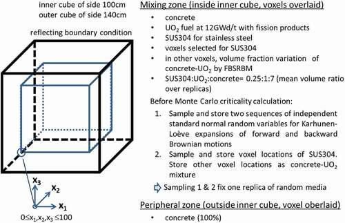
In this section, numerical results are shown for a model of concrete–UO₂ debris with stainless steel precipitates. The model geometry is the same as that appeared in previous work [2]; as shown in Figure 8, a cube of 100 × 100 × 100 cm³ is situated at the center of a cube of 140 × 140 × 140 cm³ with their corresponding faces parallel to each other. The inner cube is a mixing zone and the surrounding peripheral part is occupied by concrete. In the mixing zone, concrete and UO₂ are continuously mixed, while stainless steel precipitates in a discrete manner. This discrete treatment is different from that of previous work [2] where stainless steel was also mixed continuously with concrete and UO₂.

Figure 8. Concrete–UO₂ and stainless steel debris model.

4.1. Preliminary performance analysis of voxels and delta-tracking

The precipitates are handled by voxels and delta-tracking [23]. The computational efficiency of this handling is demonstrated for a cube of 140 × 140 × 140 cm³ consisting of concrete and UO₂ fuel at 12 GWd/t (5.0 wt% initial ²³⁵U enrichment) with the mean volume ratio of (concrete):(UO₂) = 7:1. The one-group cross sections with isotropic scattering in previous work [2] were used. The schematic description of particle tracking through voxels is shown in Figure 9 and the numerical result for its performance is shown in Figure 10. It is seen that the elimination of boundary crossing checks and the binary search through voxel indices significantly enhance the efficiency of calculation as appeared in the log-linear growth of computational time with respect to memory usage. Note that the above analysis was solely intended to examine the performance of the delta-tracking with the binary search through voxel indices. Therefore, the computation in Figure 10 was conducted without stainless steel precipitates and the Case 1 in Figure 9 always occurred as a result of the identification of the destination voxel index. As explained in the next subsection, the computations in Figures 11 and 12 were conducted with stainless steel precipitates.

Figure 9. Delta-tracking in voxels.

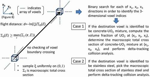
Figure 10. Performance evaluation of delta-tracking through voxels with binary search.

Figure 11. Effective multiplication factor (k_eff) over replicas of the continuously varying concrete–UO₂ medium constructed by forward–backward-superposed reflection Brownian motion containing randomly distributed voxels of stainless steel of size 1 × 1 × 1 cm³; 100 terms in Karhunen–Loève expansion in each of forward and backward Brownian motions; in each replica, 1000 initial generations discarded, followed by 4000 active generations, and 40,000 particles per generation.

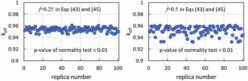
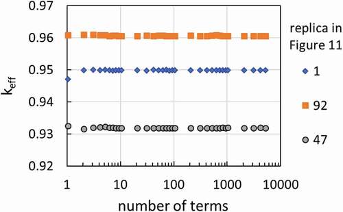
Figure 12. Neutron effective multiplication factor (k_eff) versus number of terms in Karhunen–Loève expansion for three replicas in right sub-figure (f = 0.5) in Figure 11.

4.2. Test problem description and cross section generation

The test problem is shown in Figure 8. Table 1 lists two-group cross sections computed by MVP [24]. Here, the group energy boundary was taken to be 4.5 eV because this energy is the upper limit of thermal up-scattering in MVP and is sufficiently away from the resonance peak of ²³⁸U at 6.67 eV and the gigantic resonance peak of ²⁴⁰Pu at 1.06 eV. The isotopic abundances based on SUS304 data [25] were employed for stainless steel. The material data in Ref [10] were employed for concrete and UO₂ fuel at 12 GWd/t (5.0 wt% initial ²³⁵U enrichment). The geometry and material assignment in the calculation of two-group cross sections by MVP were as follows. For SUS304, UO₂ and concrete in the mixing zone, cubes of 1 × 1 × 1 cm³, 1.077217 × 1.077217 × 1.077217 cm³, and 2.020620 × 2.020620 × 2.020620 cm³ were set up with the common center and their corresponding faces parallel to each other. These cubes define the inner, middle, and outer regions with the volume ratio of 1:0.25:7 because 1³ = 1, 1.077217³–1 = 0.25, and 2.020620³–1.077217³ = 7. UO₂, SUS304, and concrete were assigned in that order to the inner, middle, and outer regions. Specular reflection was applied to the exterior surface of the cube 2.020620 × 2.020620 × 2.020620 cm³. The cross sections computed for the inner, middle, and outer regions are the cross sections of UO₂, SUS304, and concrete in the mixing zone in Figure 8. For concrete in the peripheral zone, cubes of 1 × 1 × 1 cm³, 2 × 2 × 2 cm³, and 3 × 3 × 3 cm³ were set up with the common center and their corresponding faces parallel to each other. UO₂, concrete, and concrete were assigned in that order to the inner, middle, and outer regions. The cross sections computed for the outer region are the cross sections of concrete in the peripheral region in Figure 8. It is seen in Table 1 that the thermal-group cross sections significantly differ for concretes in the mixing and peripheral zones. All these calculations by MVP were carried out using JENDL 4.0 libraries [26].

Table 1. Two-group cross sections of concrete, UO₂, and stainless steel (T: total, A: absorption, C: capture, F: fission, ν: mean number of neutrons released per fission, S: scattering)

Location		Mixing zone (inside inner cube)			Peripheral zone
Material		UO2 ^a	Concrete	SUS304	Concrete
Epithermal (group 1)	ΣT,1	0.43760	0.39080	1.04822	0.38962
	ΣA,1	0.03282	0.00030	0.00398	0.00031
	ΣC,1	0.02495	0.00030	0.00398	0.00031
	νΣF,1	0.02040	0.0	0.0	0.0
	ΣS,1→1 ^b	0.40402	0.37924	1.04236	0.37608
	ΣS,1→2 ^b	0.00076	0.01126	0.00188	0.01323
Thermal (group 2)	ΣT,2	0.71865	0.69644	1.34126	0.79054
	ΣA,2	0.31838	0.00523	0.13289	0.00722
	ΣC,2	0.12258	0.00523	0.13289	0.00722
	νΣF,2	0.49878	0.0	0.0	0.0
	ΣS,2→1 ^b	0.00003	0.00001	0.00008	0.0
	ΣS,2→2 ^b	0.40024	0.69120	1.20829	0.78332

^a 12 GWd/t, 5.0 wt% initial ²³⁵U enrichment;

^b isotropic scattering.

In the MC criticality calculation of the model in Figure 8, voxels were overlaid and particle tracking was conducted as shown in Figure 9. Voxels in the mixing zone are randomly and independently selected for stainless steel (SUS304) and concrete–UO2 media, respectively, with the ratio of 0.25:(1 + 7) = 1:32. The selection of voxels was made before MC calculation. Two independent sequences of standard normal random variables were also sampled for FBSRBM before MC calculation. In other words, a replica of random media was created, that replica was fixed, and MC criticality calculation was conducted. The process of replica creation and subsequent MC criticality calculation was repeated many times to evaluate the fluctuation of k_eff due to the uncertainty inherent in random media formation. The voxels in the peripheral zone were always assigned concrete. When the destination of particle movement during delta-tracking was in the voxels for concrete–UO₂ media, volume fractions of concrete and UO₂ were computed using FBSRBM and KLE, cross sections were determined, and the collision processing specific to delta-tracking was carried out based on the non-analog technique by Spanier [23]. The cross section for the sampling of distance to next collision was simply chosen as the maximum total cross section over four materials in Table 1, i.e. the total cross section of SUS304. The cross section determined in this way is always larger than the cross section of any mixture of materials under consideration.

The details of the cross section computation at the voxels for concrete–UO₂ media in the mixing zone are described as follows. First, upon collision, ${\hat{B}}_M^F(x)$ and ${\hat{B}}_M^B(1-x)$ were computed using KLE. Second, setting the initial value of $\hat{F}(x)$ as ${\hat{B}}_M^F(x)+{\hat{B}}_M^B(1-x)$, the final value of $\hat{F}(x)$ was computed with $\epsilon =3$ in Algorithm (Reflection). This means that the likelihood of reflection is 1% for any x. Finally, the cross sections are assigned as:

(43) $\begin{array}{l}{\Sigma }_R(x_1,x_2,x_3)=[1-(1/8)(1+f(1/\epsilon )\widehat{F}(x_1/100))]{\Sigma }_R^{Concrete},\\ +(1/8)(1+f(1/\epsilon )\widehat{F}(x_1/100)){\Sigma }_R^{U{O}_2}\end{array}$(43)

where S denotes cross section, the subscript R stands for reaction type, f is a constant satisfying $0\le f\le 1$, 1/8 is the mean volume ratio of UO₂ in concrete–UO₂ media, the superscript of S on the right-hand side corresponds to material, and $(x_1,x_2,x_3)$ are coordinates values in Figure 8. Note that:

(44) $0\le (1/\epsilon )\left|\hat{F}(x_1/100)\right|\le 1$(44)

and $(1/8)f(1/\epsilon )\hat{F}(x_1/100)$ is the space-dependent part of the volume fraction of UO₂ in concrete–UO₂ media. This yields:

(45) $(1/8)(1-f)\le \left[\begin{array}{c}\mathrm{U}{\mathrm{O}}_2\mathrm{v}\mathrm{o}\mathrm{l}\mathrm{u}\mathrm{m}\mathrm{e}\mathrm{f}\mathrm{r}\mathrm{a}\mathrm{c}\mathrm{t}\mathrm{i}\mathrm{o}\mathrm{n}\mathrm{i}\mathrm{n}\\ \mathrm{c}\mathrm{o}\mathrm{n}\mathrm{c}\mathrm{r}\mathrm{e}\mathrm{t}\mathrm{e}-\mathrm{U}{\mathrm{O}}_2\mathrm{m}\mathrm{e}\mathrm{d}\mathrm{i}\mathrm{a}\end{array}\right]\le (1/8)(1+f)$(45)

Only the spatial variation in x₁-direction was considered, although MC criticality calculation was conducted in three-dimensions.

4.3. Numerical results for k_eff

Numerical results are shown for cases where voxels of size 1 × 1 × 1 cm³ were overlaid in Figure 8, f = 0.25 and 0.5 in Equation (43)(43) $\begin{array}{l}{\Sigma }_R(x_1,x_2,x_3)=[1-(1/8)(1+f(1/\epsilon )\widehat{F}(x_1/100))]{\Sigma }_R^{Concrete},\\ +(1/8)(1+f(1/\epsilon )\widehat{F}(x_1/100)){\Sigma }_R^{U{O}_2}\end{array}$(43) , and the first 100 terms in KLE were computed for each of ${\hat{B}}_M^F(x)$ and ${\hat{B}}_M^B(x)$ in the initial value assignment to $\hat{F}(x_1/100)$. Figure 11 shows k_eff for 100 replicas of the random media in the mixing zone in Figure 8. Each replica creation in two sub-figures in Figure 11 used the same sequence of random numbers. In other words, a sequence of random numbers in the replica m creation on left (f = 0.25 in Equation (43)(43) $\begin{array}{l}{\Sigma }_R(x_1,x_2,x_3)=[1-(1/8)(1+f(1/\epsilon )\widehat{F}(x_1/100))]{\Sigma }_R^{Concrete},\\ +(1/8)(1+f(1/\epsilon )\widehat{F}(x_1/100)){\Sigma }_R^{U{O}_2}\end{array}$(43) ) is the same as a sequence of random numbers in the replica m creation on right (f = 0.5 in Equation (43)(43) $\begin{array}{l}{\Sigma }_R(x_1,x_2,x_3)=[1-(1/8)(1+f(1/\epsilon )\widehat{F}(x_1/100))]{\Sigma }_R^{Concrete},\\ +(1/8)(1+f(1/\epsilon )\widehat{F}(x_1/100)){\Sigma }_R^{U{O}_2}\end{array}$(43) ). It is seen that the fluctuation over replicas is non-negligible and increases as f increases. The p-value in the normality test of Shapiro–Wilk [13] extended by Royston [14] indicates that the distribution of k_eff’s does not follow the normal distribution. This result can be attributed to the employment of a near-optimal neutron moderation condition concerning the volume fractions of concrete:UO₂ = 7:1 [10]; the indication of upper limit due to such an optimality is more apparent in the large fluctuation on right (f = 0.5). MC calculation for each replica consisted of 5000 generations and 40,000 particles per generation with the initial 1000 generations discarded. The standard deviation of k_eff was computed for each replica by orthonormally weighted standardized time series [27], turned out to be about 0.00005–0.00010, and thus was smaller than the marker sizes. Figure 12 shows k_eff versus the number of terms in KLE for replica 1, 92, and 47 in Figure 11 where replica 1, 92, and 47 yielded a middle value, the largest value, and the smallest value among 100 replicas. Here, it is to be noted that one term in KLE means one term in KLE for each of forward and backward BMs, i.e. two terms. It is clearly seen that the first 10 terms are sufficiently enough to ensure the reliability of k_eff calculation. Upon close inspection, the maximum and minimum k_eff values for the number of terms larger than or equal to 10 are 0.95024 ± 0.00007 and 0.95007 ± 0.00006 for replica 1, 0.96107 ± 0.00007 and 0.96077 ± 0.00007 for replica 92, and 0.93225 ± 0.00006 and 0.93207 ± 0.00007 for replica 47. Here, these errors are standard deviation. For the maximum–minimum pairs among 23 computed k_eff values for numbers of terms larger than or equal to 10, two-σ error bars contain common values for replicas 1 and 47, and three-σ error bars do the same for replica 92. Such fast-converging behaviors of k_eff for KLE approximations may be attributed to the global balance nature of k_eff, the integrated error minimality mentioned at the end of Section 3, the superposition of forward and backward BMs, and the inverse-square decrease in the eigenvalues of BM covariance function. However, the theoretical investigation of their combined effect is beyond the scope of the present work. Since the results in Figure 12 indicate that 10 terms in KLE are enough for MC criticality calculation, it is possible to significantly reduce the number of terms in KLE from 100 and implement three-dimensional cross section variation as:

(46) $\begin{array}{rl}& {\mathrm{\Sigma }}_R(x_1,x_2,x_3)=[1-(1/8)(1+f(1/3\epsilon )({\hat{F}}_1(x_1/100)\\ & +{\hat{F}}_2(x_2/100)+{\hat{F}}_3(x_3/100)))]{\mathrm{\Sigma }}_R^{Concrete}\\ & +(1/8)(1+f(1/3\epsilon )({\hat{F}}_1(x_1/100)\\ & +{\hat{F}}_2(x_2/100)+{\hat{F}}_3(x_3/100))){\mathrm{\Sigma }}_R^{U{O}_2}\end{array}$(46)

where the subscripts 1, 2, and 3 in $\hat{F}$ imply three independent computations of $\hat{F}$ by Algorithm (Reflection).

5. Conclusion and future work

In the present work, a practically implementable method was developed for the modeling of random media using the bounded fluctuation driven by normal noise. The method is free of log-normal transformation, utilizes the superposition of forward and backward BM with path reflection, and is applicable to the fluctuation with upper and lower bounds. The method has been termed FBSRBM, and it is possible to efficiently implement FBSRBM by the KLE of stochastic processes [8,9]. FBSRBM was applied to the space-dependent fluctuation of the volume fractions of UO₂–concrete media in a system comprised of UO₂, concrete, and stainless steel. Numerical results for k_eff demonstrate the uncertainty of k_eff due to the uncertainty inherent in debris formation. Therefore, FBSRBM is a valuable media randomization tool in MC criticality analysis under material distribution uncertainty in addition to the RWF developed previously [2]. The mathematical methodology in FBSRBM is sufficiently general and can be adapted and further developed to model other randomization techniques. Surface randomization will be an important next-step research endeavor in terms of criticality safety in debris drilling.

BM is a special case of fractional Brownian motion (FBM) which covers a wide range of correlation functions [11]. It is thus natural to proceed to the random media modeling with FBM. The challenging issue will be the analytical unsolvability of the eigenvalue problem of FBM covariance function except for the special case of BM. An approximation other than KLE should be sought after. To this end, it will be worth investigating practical use of the wavelet expansion of FBM [19].

Acknowledgments

Work reported in this paper was performed under the auspices of Secretariat of Nuclear Regulation Authority (S/NRA/R) of Japan. The author is thankful to Dr. K Tonoike, Nuclear Safety Research Center, Japan Atomic Energy Agency, for the support of Monte Carlo methodology development.

Disclosure statement

No potential conflict of interest was reported by the author.

References

- Cover TM, Thomas JA. Elements of information theory. 2nd ed. Hoboken, NJ (USA): John-Wiley & Sons; 2006.
- Ueki T. Monte Carlo criticality analysis under material distribution uncertainty. J Nucl Sci Technol. 2017;54:267–279.
- Olson AJ, Prinja AK, Franke BC. Radiation transport in random media with large fluctuations. Trans Am Nucl Soc. 2016;114:357–360.
- Durrett R. Probability: theory and examples. 2nd ed. Belmont CA (USA): Wadsworth Publishing Company; 1996.
- Karatzas I, Shreve SE. Brownian motion and stochastic calculus. 2nd ed. New York NY (USA): Springer; 1998.
- Meterelliyoz M, Alexopoulos C, Goldsman D, et al. Reflected variance estimators for simulation. IIE Trans. 2015;47:1185–1202.
- Ueki T. A power spectrum approach to tally convergence in Monte Carlo criticality calculation. J Nucl Sci Technol. 2017;54:1310–1320.
- Ghanem RG, Spanos PD. Stochastic finite elements: a spectral approach. New York NY (USA): Springer-Verlag; 1991.
- Sullivan TJ. Introduction to uncertainty quantification. Cham (Switzerland): Springer International Publishing AG; 2015.
- Izawa K, Uchida Y, Ohkubo K, et al. Infinite multiplication factor of low-enriched UO2-concrete system. J Nucl Sci Technol. 2012;49:1043–1047.
- Mandelbrot BB, Van Ness JW. Fractional Brownian motion, fractional noises and applications. SIAM Rev. 1968;10(4): 422–437. Reprint in Mandelbrot BB. Gaussian Self-Affinity and Fractals. New York NY (USA): Springer-Verlag; 2002.
- Reed IS, Lee PC, Truong TK. Spectral representation of fractional Brownian motion in n dimensions and its properties. IEEE Trans Inf Theory. 1995;41(5):1439–1451.
- Shapiro SS, Wilk MB. An analysis of variance test for normality (complete samples). Biometrika. 1965;52(3 and 4):591–611.
- Royston JP. An extension of Shapiro and Wilk’s W test for normality to large samples. J Royal Stat Society. Ser C (Applied Statistics). 1982;31(2):115–124.
- Williams MMR. Polynomial chaos functions and stochastic differential equations. Ann Nucl Energy. 2006;33:774–785.
- Park S, Williams MMR, Prinja AK, et al. Modelling non-Gaussian uncertainties and the Karhunen-Loève expansion within the context of polynomial chaos. Ann Nucl Energy. 2015;76:146–165.
- Jorgensen PET. Analysis and probability: wavelets, signals, fractals. New York NY (USA): Springer-Verlag; 2006.
- Raymond A. Euler and the Zeta function. Am Math Monthly. 1974;81(10):1067–1086.
- Meyer Y, Sellan F, Taqqu MS. Wavelets, generalized white noise and fractional integration: the synthesis of fractional Brownian motion. J Fourier Anal Appl. 1999;5(5):465–494.
- Dzhaparidze K, Van Zanten H, Series A. Expansion of fractional Brownian motion. Probab Theory Rel. 2004;130:39–55.
- Matsumoto H, Taniguchi S. Stochastic analysis: Ito and Malliavin calculus in tandem. New York NY (USA): Cambridge University Press; 2017.
- Yajima K. Lebesgue integral and functional analysis. New ed. Shinjyuku, Tokyo (JPN): Asakura-Syoten; 2015. in Japanese.
- Spanier J. Two pairs of families of estimators for transport problems. SIAM J Appl Math. 1966;14(4):702–713.
- Nagaya Y, Okumura K, Mori T, et al. MVP/GMVP II: general purpose Monte Carlo codes for neutron and photon transport calculations based on continuous energy and multigroup methods. Tokai-mura, Ibaraki-ken (Japan): Japan Atomic Energy Agency; 2005. ( JAERI-1348).
- Okuno H, Suyama K, Tonoike K, et al. Second version of data collection part of nuclear criticality safety handbook. Japan: Japan Atomic Energy Agency; 2009. ( JAEA-Data/Code 2009-010 [in Japanese]).
- Shibata K, Iwamoto O, Nakagawa T, et al. JENDL-4.0: a new library for nuclear science and engineering. J Nucl Sci Technol. 2011;48(1):1–30.
- Ueki T. An orthonormally weighted standardized time series for the error estimation of local tallies in Monte Carlo criticality calculation. Nucl Sci Eng. 2012;171:220–230.