Development of drift–flux correlation for predicting void fraction in downcomer regions

ABSTRACT

Accurate prediction of interfacial drag in the downcomer annulus is crucial for the assessment of downcomer void fraction for the loss of coolant accident analysis. The downcomer annulus is the gap between reactor pressure vessel (RPV) exterior and the inner wall of pressure containment vessel (PCV). Based on the previous research, occurrence of the nonuniform two-phase flow in downcomer section is reported, which is partly due to the large wall temperature difference between RPV exterior and the inner wall of PCV. In RELAP5, interfacial drag term in downcomer section is calculated using Kataoka–Ishii and churn-turbulent drift–flux correlations. It has been pointed out that this traditional calculation approach for calculating downcomer void fraction needs modification. The purpose of the current study is to assess the behaviors of drift–flux parameters in downcomer section and to propose an improved distribution parameter model that is suitable for donwcomer boiling analysis.

KEYWORDS:

• Thermal-hydraulics
• drift–flux model
• void fraction
• downcomer

1. Introduction

Gas–liquid two-phase flow is a commonly observed phenomenon in various engineering disciplines such as chemical processing, heat exchanging systems, nuclear power generation. In nuclear engineering, accurate predictions of two-phase parameters are crucial to ensure safety of the nuclear power plants. In order to accurately predict the phenomenon, reactor safety analysis code, such as RELAP5 [1], is often utilized to conduct systematic safety analysis of reactor components. However, predictive capability of the computational code is heavily dependent on the selection of appropriate transport equations and constitutive equations. Hence, it is crucial to utilize appropriate formulations to conduct safety analysis that is physical and accurate [2, 3].

In advanced pressurized water reactor, understanding of the downcomer boiling (DOBO) phenomena is crucial to predict the transient behavior of a postulated small-break loss of coolant accident (SBLOCA), or the reactor coolant pump (RCP) coast down, while the emergency core coolant (ECC) water is injected into the reactor unit. It is known that sudden boiling is induced in the downcomer region due to the nonuniform heating within the channel, and this results in circulating two-phase flow pattern DOBO as can be seen from Figure 1 [4]. Nonuniform void fraction profile is generated due to the nonuniform heating and recirculatory flow behavior near the flow inlet. Vapor generation in downcomer region will heavily influence the hydraulic head of the coolant, which eventually affects the coolant injection rate of the reactor core during SBLOCA or RCP coast down. In the worst-case scenario, it could result in the failure of reactor core.

Figure 1. Illustration of Downcomer boiling two-phase flow characteristics [4].

According to the previously conducted DOBO analysis using RELAP5 code, the output results overestimated the void fraction value in downcomer region [4–6]. The possible cause of the overestimation is due to the drift–flux models utilized in the code such as Ishii’s churn flow model [7] and Kataoka–Ishii’s model [8] that are not capable of resolving highly nonuniform phase distribution observed in DOBO. In addition, interfacial shear model utilized in the current RELAP5 code may not be suitable for DOBO. Based on the aforementioned issues, the purpose of this study is to newly develop drift–flux correlations that can accurately predict thermal-hydraulic behaviors for DOBO.

2. DOBO experiment

Currently available DOBO experimental database is from the one conducted at Korea Atomic Energy Research Institute (KAERI) simulating the ECC injection phenomena during large break LOCA [4]. Schematic of the experimental facility is shown in Figure 2. The test section is comprised of 5.1 m tall heating channel and 0.25 m width of the rectangular flow channel simulating the downcomer region. The test section width is identical to that of APR 1400, but the volume and flow area are scaled down to 1/47.08. To simulate the ECC injection, direct vessel injection (DVI) port of 1.0 m long is installed on top of the heated section and 0.3 m long drain port is installed at the bottom of the test section. Heat flux of the test section was adjusted to simulate the APR1400’s heated surface wall conditions, and 1.33 kg/s of simulated ECC water flow (scaled down by 47.08) was injected into the test section for the experiment. Their experimental conditions are tabulated in Table 1. Area averaged void fraction measurement was conducted at seven different axial locations and five of them were conducted at the heated channel. Five-conductance probes with traversing unit were utilized to conduct the void fraction measurement with accuracy of 6.1%.

Table 1. Test conditions of KAERI’s downcomer boiling experiment [4]

Parameter	TECC (°C)	Psys (kPa)	WECC (kg/s)	q″ (kW/m^2)
R1	110.1	162.8	1.22	50.2
R2	110.2	161.4	1.16	69.7
R3	109.6	166.5	1.20	82.1
R4	109.5	170.8	1.20	91.1
R2-1a	110.7	158.5	1.33	70.5

Figure 2. Downcomer boiling experimental facility [4].

The obtained axial average void fraction trend with respect to the elevation and surface wall heat flux is shown in Figure 3. As can be seen from the trend, void fraction is negligibly small below the elevation of 2.8 m, but it tends to largely increase beyond that point. It is reported that the RELAP5 calculation overestimated the void fraction value for more than 40% in this region [6]. This result shows the importance of improving the constitutive equations utilized in RELAP5 calculation. The authors concluded the necessity to improve the interfacial friction coefficients utilized in RELAP5, and that may improve the predictive capability of void fraction in downcomer channel.

Figure 3. Axial void fraction data on downcomer boiling [4].

3. Constitutive equations of RELAP5/MOD3 code

In RELAP5/MOD3.2 code, drift–flux model [9] is utilized to calculate the interfacial drag term for both bubbly and slug flow regimes in vertical orientation. Drift–flux model is one of the significant models available in safety analysis codes for predicting area-averaged void fraction values.

3.1. Drift–flux model

Drift–flux model is commonly used to calculate area-averaged void fraction <α> by using constitutive relations for drift velocity $⟨⟨V_{gj}⟩⟩$ and distribution parameter C₀, which is a covariance between phase distribution and volumetric flux. It is generally expressed as follows:

(1) $\frac{⟨j_g⟩}{⟨\alpha ⟩}=⟨⟨v_g⟩⟩=C_0⟨j⟩+⟨⟨V_{gj}⟩⟩$(1)

Here, <j_g>, <j>, $⟨⟨V_g⟩⟩$ are the superficial gas velocity, total superficial velocity, and gas velocity, respectively. The distribution parameter C₀ and drift velocity $⟨⟨V_{gj}⟩⟩$ are defined by the following relations:

(2) $C_0=\frac{⟨\alpha j⟩}{⟨\alpha ⟩⟨j⟩}$(2)

(3) $⟨⟨V_{gj}⟩⟩=\frac{⟨\alpha V_{gj}⟩}{⟨\alpha ⟩}$(3)

where V_gj is the local drift velocity which is typically defined as V_gj = v_g-j. The brackets <> and ≪ ≫ represent area-averaging and void-weighted area averaging, respectively. In general, measurement data points are plotted on $⟨j⟩-⟨⟨v_g⟩⟩$ plane to evaluate drift–flux parameters. In the plane, the distribution parameter C₀ and drift velocity $⟨⟨V_{gj}⟩⟩$ values are determined from the slope and y-axis intersection point. This methodology is appropriate for the experiment conducted under fully developed two-phase flow conditions. In the case where database obtained at undeveloped flow conditions is utilized, the drift–flux correlations may contain compensation error that cannot be neglected. As an example, uncertainties in $⟨⟨V_{gj}⟩⟩$ may be possibly hidden by utilizing the underestimated C₀ correlation in Equation (1)(1) $\frac{⟨j_g⟩}{⟨\alpha ⟩}=⟨⟨v_g⟩⟩=C_0⟨j⟩+⟨⟨V_{gj}⟩⟩$(1) . Hence, the drift–flux correlations should be developed independently using Equations (2)(2) $C_0=\frac{⟨\alpha j⟩}{⟨\alpha ⟩⟨j⟩}$(2) and (3(3) $⟨⟨V_{gj}⟩⟩=\frac{⟨\alpha V_{gj}⟩}{⟨\alpha ⟩}$(3) ).

In RELAP5/MOD3.2 code, drift–flux model is utilized to calculate the interfacial drag term for both bubbly and slug flow regimes in vertical orientation. The constitutive relation for the interfacial drag term calculated in this manner is necessary to close momentum equation in two-fluid model. Here, generalized interfacial drag FI is defined using the interfacial drag term F_i as follows:

(4) $FI=\frac{\frac{F_i}{⟨\alpha ⟩{\rho }_g}+\frac{F_i}{\left(1-⟨\alpha ⟩\right){\rho }_f}}{{\rho }_m⟨v_r⟩}$(4)

Here, variable ρ_f, ρ_g, ρ_m, v_r are liquid-phase density, gas-phase density, two-phase mixture density, and relative velocity, respectively. The interfacial drag term F_i is defined using following relation:

(5) $F_i=C_i\left|⟨v_r⟩\right|⟨v_r⟩$(5)

C_i terms utilized in Equation (5)(5) $F_i=C_i\left|⟨v_r⟩\right|⟨v_r⟩$(5) are interfacial drag coefficient. Relative velocity and interfacial drag coefficient are defined as shown in Equations (6)(6) $⟨v_r⟩=C_1⟨⟨v_g⟩⟩-C_0⟨⟨v_f⟩⟩$(6) and (7).

(6) $⟨v_r⟩=C_1⟨⟨v_g⟩⟩-C_0⟨⟨v_f⟩⟩$(6)

(7) $C_i=\frac{⟨\alpha ⟩{\left(1-⟨\alpha ⟩\right)}^3\left({\rho }_f-{\rho }_g\right)gsin\varphi }{\left|⟨⟨V_{gj}⟩⟩\right|⟨⟨V_{gj}⟩⟩}$(7)

Here, g and ϕ are gravitational acceleration and inclination angle, respectively. The C₁ term in Equation (6)(6) $⟨v_r⟩=C_1⟨⟨v_g⟩⟩-C_0⟨⟨v_f⟩⟩$(6) is defined as shown in Equation (8)(8) $C_1=\frac{1-C_0⟨\alpha ⟩}{1-⟨\alpha ⟩}$(8) .

(8) $C_1=\frac{1-C_0⟨\alpha ⟩}{1-⟨\alpha ⟩}$(8)

Table 2 tabulates the drift–flux correlations for bubbly and slug flow regimes utilized in RELAP5/MOD3.2 code. In typical PWR downcomer section, the channel gap ranges from 0.10 to 0.25m, and it is treated as large diameter pipe in RELAP5. For the large diameter pipe (D > 8.0 cm), correlations proposed by Kataoka–Ishii and Ishii’s churn flow model (hereafter, ‘Ishii–Churn correlation’) are utilized, and they are also utilized for the DOBO analysis in RELAP5.

Table 2. Drift–flux correlations utilized in RELAP5/MOD3.2 code for bubbly and slug flow regimes (RELAP5 Manual)

Flow rates	Rod bundles	Small pipes D < 0.018 m	Intermediate pipes 0.018 m< D < 0.08 m	Large pipes 0.08 m < D
High upflow rates G > 100 Kg/m^2•s	EPR I(2) (eprij)	EPRI (3) (eprij)	EPRI (9) (eprij)	Clum turbulent bubbly flow (14) transition (15) Koltaoka–Ishii(16) (katokj)
		Transition (5)	Transition (13)
Low up, down, and countercurrent flow rates G < 50 Kg/m^2•s G > −50 Kg/m^2•s		Zuber–Findaly slug flow (4) (zfslgi)	Clum turbulent bubbly flow (10) transition (11) Koltaoka–Ishii (12) (katokj)
		Transition (5)	Transition (13)
High downflow rates G<-100 kg/m^2•s		EPRI (3) (eprij)	EPRI (9) (eprij)

3.2. Distribution parameters

As documented in RELAP5 manual, the C₀ is dependent on void fraction and density ratio, and typically evaluated using two different approaches shown in following equations:

(9) $C_0=\left[C_{\mathrm{\infty }}-\left(C_{\mathrm{\infty }}-1\right)\sqrt{\frac{{\rho }_f}{{\rho }_g}}\right]\left(1-e^{-18\alpha }\right)\mathrm{f}\mathrm{o}\mathrm{r}\alpha \le 0.8$(9)

and

(10) $C_0=5\left(\alpha -0.8\right)+\left(1-\alpha \right)\left[C_{\mathrm{\infty }}-\left(C_{\mathrm{\infty }}-1\right)\sqrt{\frac{{\rho }_f}{{\rho }_g}}\right]\left(1-e^{-18\alpha }\right)\mathrm{f}\mathrm{o}\mathrm{r}\alpha >0.8$(10)

When neglecting void generation near-wall region, Equation (9)(9) $C_0=\left[C_{\mathrm{\infty }}-\left(C_{\mathrm{\infty }}-1\right)\sqrt{\frac{{\rho }_f}{{\rho }_g}}\right]\left(1-e^{-18\alpha }\right)\mathrm{f}\mathrm{o}\mathrm{r}\alpha \le 0.8$(9) can be simplified to Equation (11)(11) $C_0=C_{\mathrm{\infty }}-\left(C_{\mathrm{\infty }}-1\right)\sqrt{\frac{{\rho }_f}{{\rho }_g}}\mathrm{f}\mathrm{o}\mathrm{r}\alpha \le 0.8$(11) .

(11) $C_0=C_{\mathrm{\infty }}-\left(C_{\mathrm{\infty }}-1\right)\sqrt{\frac{{\rho }_f}{{\rho }_g}}\mathrm{f}\mathrm{o}\mathrm{r}\alpha \le 0.8$(11)

Here, modified version of Kataoka–Ishii’s correlation, also known as modified Rouhani’s correlation, is utilized for the C₀ in DOBO analysis and its C_∞ is defined as follows:

(12) $C_{\mathrm{\infty }}=1+0.2{\left(\frac{{\rho }_f\sqrt{gD}}{\left|G\right|+0.001}\right)}^{0.5}$(12)

The mass flux G is defined as follows:

(13) $\left|G\right|=\alpha {\rho }_g\left|v_g\right|+(1-\alpha ){\rho }_f\left|v_f\right|$(13)

The distribution parameter utilized in RELAP5 was originally developed for upward two-phase flow conditions, which does not consider the recirculatory flow pattern in DOBO. As can be seen from Figure 1, void fraction distribution in downcomer channel greatly differs from the symmetric distribution seen in the upward pipe flow case. Hence, the development of the distribution parameter for DOBO is crucial for the accurate physical representation of downcomer two-phase flow.

3.3. Drift velocity

For the drift velocity correlation, dimensionless drift velocity V_gj⁺ is utilized for the analysis.

(14) $⟨⟨V_{gj}^{+}⟩⟩=\frac{⟨⟨V_{gj}⟩⟩}{{\left(\frac{\sigma g\mathrm{\Delta }\rho }{{\rho }_f^2}\right)}^{0.25}}$(14)

Here, the bracket ≪≫ represents void-weighted average value. Kataoka–Ishii’s correlation for V_gj⁺ is dependent on fluid physical properties and channel diameter, and is given as follows:

(15) $V_{gj}^{+}=0.0019{\left(D^{\ast }\right)}^{0.809}{\left(\frac{{\rho }_g}{{\rho }_f}\right)}^{-0.157}{N}_{\mu f}^{-0.157}\mathrm{f}\mathrm{o}\mathrm{r}{D}^{\ast }\le 30$(15)

and

(16) $V_{gj}^{+}=0.030{\left(\frac{{\rho }_g}{{\rho }_f}\right)}^{-0.157}{N}_{\mu f}^{-0.562}\mathrm{f}\mathrm{o}\mathrm{r}{D}^{\ast }>30$(16)

Here, D*, N_μ,σ are respectively, the Bond number of hydraulic diameter, dimensionless viscosity number, and surface tension. Equations (15)(15) $V_{gj}^{+}=0.0019{\left(D^{\ast }\right)}^{0.809}{\left(\frac{{\rho }_g}{{\rho }_f}\right)}^{-0.157}{N}_{\mu f}^{-0.157}\mathrm{f}\mathrm{o}\mathrm{r}{D}^{\ast }\le 30$(15) and (16(16) $V_{gj}^{+}=0.030{\left(\frac{{\rho }_g}{{\rho }_f}\right)}^{-0.157}{N}_{\mu f}^{-0.562}\mathrm{f}\mathrm{o}\mathrm{r}{D}^{\ast }>30$(16) ) are applicable for the fluids that satisfy the dynamic viscosity condition of $N_{\mu f}\le 2.25\times {10}^{-3}$. For the fluid that exceeds this value, following drift velocity correlation is utilized in the code.

(17) $V_{gj}^{+}=0.92{\left(\frac{{\rho }_g}{{\rho }_f}\right)}^{-0.157}\mathrm{f}\mathrm{o}\mathrm{r}{D}^{\ast }>30$(17)

where D* and $N_{\mu f}$ are defined as follows:

(18) $D^{\ast }=D\sqrt{\frac{g\left({\rho }_f-{\rho }_g\right)}{\sigma }}$(18)

(19) $N_{{\mu }_f}=\frac{{\mu }_f}{{\left({\rho }_f\sigma \sqrt{\frac{\sigma }{g({\rho }_f-{\rho }_g)}}\right)}^{1/2}}$(19)

For Ishii–Churn correlation in RELAP5/MOD3.2, following drift velocity relation is utilized:

(20) $⟨⟨V_{gj}⟩⟩=\sqrt{2}{\left(\frac{\sigma g\mathrm{\Delta }\rho }{{\rho }_f^2}\right)}^{0.25}$(20)

The transition from Ishii–Churn correlation to Kataoka–Ishii’s correlation takes place when the dimensionless superficial gas velocity <j_g⁺> reaches 0.5, which is defined as follows:

(21) $⟨j_g^{+}⟩=\frac{⟨j_g⟩}{{\left[\frac{\sigma g\left({\rho }_f-{\rho }_g\right)}{{\rho }_f^2}\right]}^{0.25}}=⟨j_{g1}^{+}⟩=0.5$(21)

The transition to Kataoka–Ishii’s correlation ends when $⟨j_g^{+}⟩$ reaches its end-point, $⟨j_{g2}^{+}⟩$= 1.768. Hence, transition from Ishii–Churn to Kataoka–Ishii’s correlation takes place when dimensional superficial gas velocity is in the following range:

(22) $0.5<⟨j_g^{+}⟩<1.768$(22)

Within the transition range, Equation (23)(23) $⟨⟨V_{gj}^{Interpolation}⟩⟩=⟨⟨V_{gj}^{Ishii-Churn}⟩⟩+\frac{⟨⟨j_g^{+}⟩⟩-⟨⟨j_{g1}^{+}⟩⟩}{⟨⟨j_{g2}^{+}⟩⟩-⟨⟨j_{g1}^{+}⟩⟩}⟨⟨V_{gj}^{Kataoka-Ishii}⟩⟩-⟨⟨V_{gj}^{Ishii-Churn}⟩⟩$(23) is utilized as a linear interpolation function between Ishii–Churn and Kataoka–Ishii’s correlations.

(23) $⟨⟨V_{gj}^{Interpolation}⟩⟩=⟨⟨V_{gj}^{Ishii-Churn}⟩⟩+\frac{⟨⟨j_g^{+}⟩⟩-⟨⟨j_{g1}^{+}⟩⟩}{⟨⟨j_{g2}^{+}⟩⟩-⟨⟨j_{g1}^{+}⟩⟩}⟨⟨V_{gj}^{Kataoka-Ishii}⟩⟩-⟨⟨V_{gj}^{Ishii-Churn}⟩⟩$(23)

The drift velocity correlations utilized in RELAP5 is specifically developed for upward two-phase flow channel. As a result, utilization of those correlations may not be suitable for downcomer channel where highly nonuniform void faction distribution as well as the recirculatory flow pattern are observed in the channel. The drift velocity correlation developed by Hibiki and Ishii [10] considers detailed treatment including the wall shear stress term. Thus, it is applicable for wide range of inlet flow rates, as well as for the extreme flow conditions including the significant wall shear-stress on the relative velocity between phases. Hence, for the extreme flow condition observed in downcomer two-phase flow, the drift velocity correlation developed by Hibiki and Ishii [10] is expected to perform well.

4. Modifications of constitutive equations for DOBO analysis

As was mentioned in previous chapter, Equation (1)(1) $\frac{⟨j_g⟩}{⟨\alpha ⟩}=⟨⟨v_g⟩⟩=C_0⟨j⟩+⟨⟨V_{gj}⟩⟩$(1) is typically utilized to calculate area-averaged void fraction. One of the problems for utilizing C₀ correlations listed in Equations (9)(9) $C_0=\left[C_{\mathrm{\infty }}-\left(C_{\mathrm{\infty }}-1\right)\sqrt{\frac{{\rho }_f}{{\rho }_g}}\right]\left(1-e^{-18\alpha }\right)\mathrm{f}\mathrm{o}\mathrm{r}\alpha \le 0.8$(9) and (10(10) $C_0=5\left(\alpha -0.8\right)+\left(1-\alpha \right)\left[C_{\mathrm{\infty }}-\left(C_{\mathrm{\infty }}-1\right)\sqrt{\frac{{\rho }_f}{{\rho }_g}}\right]\left(1-e^{-18\alpha }\right)\mathrm{f}\mathrm{o}\mathrm{r}\alpha >0.8$(10) ) for DOBO analysis is that they were not developed for the nonuniform two-phase flow behavior.

In order to simulate a recirculatory flow pattern observed in the downcomer using one-dimensional system analysis code such as RELAP5, it is necessary to split the flow channel nodalization into two channels (upward and downward flow). Lee et al. [5] utilized two-channel nodalization approach to simulate the recirculatory flow pattern seen in DOBO. In the current study, downcomer flow channel was split into 9:1 ratio, which corresponds to upward and downward flow, respectively. This ratio was determined from the preliminary analysis using RELAP5 that best represented the DOBO experimental condition.

Here, derivation of the distribution parameter for upward flow region in the downcomer channel (i.e. wall-heated region) is described. For the sake of clarity, the area-averaged operator in the upward flow region is defined using < >_U. The general expression of drift–flux model for upward flow region can be expressed as follows:

(1)’ $\frac{{⟨j_g⟩}_U}{{⟨\alpha ⟩}_U}=C_{0,U}{⟨j⟩}_U+{⟨⟨V_{gj}⟩⟩}_U,$(1)’

Here, $C_{0,U}$ and ${⟨⟨V_{gj}⟩⟩}_U$ are the distribution parameter, and drift velocity in upward flow region, respectively, which are defined as follows:

(2)’ $C_{0,U}=\frac{{⟨\alpha j⟩}_U}{{⟨\alpha ⟩}_U{⟨j⟩}_U},$(2)’

(3)’ ${⟨⟨V_{gj}⟩⟩}_U=\frac{{⟨\alpha V_{gj}⟩}_U}{{⟨\alpha ⟩}_U}.$(3)’

4.1. Consideration of distribution parameter using BLT model

Here, C_0,U will be specifically derived for DOBO condition by assuming void fraction and superficial velocity profiles as shown in Figure 4. As can be seen from the plot, volumetric flux becomes 0 at the heated wall surface and possesses maximum value slightly away from the wall, which is consistent with the wall boiling phenomena. The present derivation resembles bubble layer thickness (BLT) concept, proposed by Hibiki et al. [11]. Here, DOBO region is mainly divided into upflow and downflow regions, where the upflow region ranges from x = 0 to L. Downflow region is assumed to be in single-phase flow. For the superficial velocity profile for upflow condition, its peak (j = j₀) is assumed to be at x = x₀. For the channel region ranging from 0 to x₀,

(24) $\frac{j}{j_0}=\frac{x}{x_0}$(24)

Figure 4. Downcomer region analysis model.

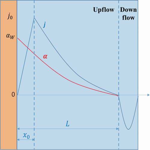
and for x₀ to L,

(25) $\frac{j}{j_0}={\left(1-\frac{x-x_0}{L-x_0}\right)}^m$(25)

The exponent m provides power-law flow profile, which can be adjusted depending on the flow condition in the channel. Likewise, the void fraction profile can be assumed that the maximum value α_w takes place at the heated wall region (x = 0) and α gradually approaches to 0 at x = L.

(26) $\frac{\alpha }{{\alpha }_w}={\left(1-\frac{x}{L}\right)}^n$(26)

The exponent n provides power-law void profile, which can be adjusted depending on the flow condition in the channel.

Then, area-averaged void fraction <α>_U and area-averaged superficial velocity <j>_U can be calculated as follows:

(27) ${⟨\alpha ⟩}_U=\frac{1}{L}\underset{0}{\overset{L}{\int }}\alpha dx=\frac{{\alpha }_W}{L}\underset{0}{\overset{L}{\int }}{\left(1-\frac{x}{L}\right)}^{n}dx=\frac{{\alpha }_W}{n+1}$(27)

(28) $⟨j{⟩}_U=\frac{1}{L}\underset{0}{\overset{L}{\int }}jdx=\frac{1}{L}\underset{0}{\overset{x_0}{\int }}jdx+\frac{1}{L}\underset{x_0}{\overset{L}{\int }}jdx=\frac{j_0{x}_0}{2L}+\frac{j_0}{m+1}$(28)

Likewise, $⟨\alpha j⟩$_U can be analytically derived, which is shown in the Equation (A9)(A9) $\begin{array}{rl}& ⟨\alpha j{⟩}_U=\frac{1}{L}\underset{0}{\overset{L}{\int }}\alpha jdx\\ & =\frac{{\alpha }_W{j}_{0}L}{x_0}\left\{\frac{1}{n+1}-\frac{1}{n+2}-\frac{{\left(1-\frac{x_0}{L}\right)}^{n+1}}{n+1}+\frac{{\left(1-\frac{x_0}{L}\right)}^{n+2}}{n+2}\right\}\\ & +\frac{{\alpha }_W{j}_0{\left(1-\frac{x_0}{L}\right)}^{n+1}}{n+m+1}\end{array}$(A9) of appendix section. Then, by following its original definition C_0,U shown in Equation (2)(2) $C_0=\frac{⟨\alpha j⟩}{⟨\alpha ⟩⟨j⟩}$(2) ’, it can be analytically calculated as,

(29) $C_{0,U}=\frac{\frac{L}{x_0}\left\{\frac{1}{n+1}-\frac{1}{n+2}-\frac{{\left(1-\frac{x_0}{L}\right)}^{n+1}}{n+1}+\frac{{\left(1-\frac{x_0}{L}\right)}^{n+2}}{n+2}\right\}+\frac{{\left(1-\frac{x_0}{L}\right)}^{n+1}}{\left(n+m+1\right)}}{\frac{1}{n+1}\left(\frac{x_0}{2L}+\frac{1}{m+1}\right)}$(29)

In order to obtain an estimate of C_0,U for DOBO condition, wall void fraction of α_w = 0.8, peak location of x₀/L = 0.1, and volumetric flow velocity profile m = 7 were considered. The change in C_0,U with respect to the area-averaged void fraction is plotted in Figure 5. For the effect of profiles m and n, n tends to be large when the area-averaged void fraction <α > _U is in low range, and C_0,U eventually approaches to 0. This is consistent with the Ishii’s constitutive equation for C₀ on subcooled boiling flow (Equation (9)(9) $C_0=\left[C_{\mathrm{\infty }}-\left(C_{\mathrm{\infty }}-1\right)\sqrt{\frac{{\rho }_f}{{\rho }_g}}\right]\left(1-e^{-18\alpha }\right)\mathrm{f}\mathrm{o}\mathrm{r}\alpha \le 0.8$(9) ). Hence, as is depicted in Figure 5, C_0,U in DOBO possesses its peak value in low void fraction range and it gradually approaches to 1.0 with respect to an increase in void fraction.

Figure 5. Distribution parameter using BLT model.

4.2. Constitutive equation for distribution parameter

In order to obtain C_0,U correlation for DOBO, inverse analysis was conducted from the experimental values. First, by utilizing the general expression of drift–flux model defined in Equation (1)(1) $\frac{⟨j_g⟩}{⟨\alpha ⟩}=⟨⟨v_g⟩⟩=C_0⟨j⟩+⟨⟨V_{gj}⟩⟩$(1) ’, C_0,U was calculated. For the drift velocity ${⟨⟨V_{gj}⟩⟩}_U$, Hibiki and Ishii’s model [10], which is applicable for the large diameter pipe of wide range of flow conditions, was utilized. Hibiki–Ishii’s drift velocity correlation is defined as follows:

(30) $\begin{array}{rl}& {⟨⟨V_{gj}^{Hibiki-Ishii}⟩⟩}_U={⟨⟨V_{gj}^{Ishii-Churn}⟩⟩}_U\\ & {\left(1-{⟨\alpha ⟩}_U\right)}^{1.75}{e}^{-1.39{⟨j_g^{+}⟩}_U}\\ & +{⟨⟨V_{gj}^{Kataoka-Ishii}⟩⟩}_U\left(1-e^{-1.39{⟨j_g^{+}⟩}_U}\right)\end{array}$(30)

In Figure 6, calculation results of C_0,U is plotted with the DOBO experimental values and the BLT model derived in previous section using x₀/L = 0.05. Due to the large measurement uncertainty for the low void fraction region, the database with void fraction values larger than 0.1 was considered for the comparison. Even though the experimental data show different trend near low void fraction region, it is physical to assume that C_0,U approaches zero as the area averaged void fraction approaches zero.

Figure 6. Newly developed distribution parameter model.

Based on the C_0,U values obtained from the inverse analysis, C_0,U correlation was developed for both low and high void fraction regions as shown in Equations (31)(31) $C_{0,U}=19.4⟨\alpha {⟩}_U-\left(19.4⟨\alpha {⟩}_U-1\right)\sqrt{\frac{{\rho }_g}{{\rho }_f}}$(31) and (32(32) $\begin{array}{rl}& C_{0,U}=\left\{1.06\times {10}^{5}exp\left[-11.8{\left\{{⟨\alpha ⟩}_U/\left(1-{⟨\alpha ⟩}_U\right)\right\}}^{0.0692}\right]+1\right\}\\ & -\left\{1.06\times {10}^{5}exp\left[-11.8{\left\{{⟨\alpha ⟩}_U/\left(1-{⟨\alpha ⟩}_U\right)\right\}}^{0.0692}\right]\right\}\\ & \sqrt{\frac{{\rho }_g}{{\rho }_f}}\end{array}$(32) ).

Low void fraction region

(31) $C_{0,U}=19.4⟨\alpha {⟩}_U-\left(19.4⟨\alpha {⟩}_U-1\right)\sqrt{\frac{{\rho }_g}{{\rho }_f}}$(31)

High void fraction region

(32) $\begin{array}{rl}& C_{0,U}=\left\{1.06\times {10}^{5}exp\left[-11.8{\left\{{⟨\alpha ⟩}_U/\left(1-{⟨\alpha ⟩}_U\right)\right\}}^{0.0692}\right]+1\right\}\\ & -\left\{1.06\times {10}^{5}exp\left[-11.8{\left\{{⟨\alpha ⟩}_U/\left(1-{⟨\alpha ⟩}_U\right)\right\}}^{0.0692}\right]\right\}\\ & \sqrt{\frac{{\rho }_g}{{\rho }_f}}\end{array}$(32)

4.3. RELAP5 analysis

Next, the drift–flux correlations developed in this study are implemented into RELAP5 code and its void fraction predictive capability was assessed with KAERI’s DOBO experimental data. The RELAP5 nodalization simulating DOBO is shown in Figure 7. The test section was divided into seven volumes corresponding to the differential pressure cells of LT-1 to LT-7 shown in Figure 3, so that the volume center positions became the void fraction evaluation positions. In KAERI’s DOBO experiment, as was explained in previous chapter, upward two-phase flow was observed near the heating surface while downward coolant flow was observed along the non-heated surface which results in nonuniform channel-wise flow pattern. In order to simulate this phenomenon, two separate flow channels for heated section and coolant injection (ECC) section were generated. As can be seen from the node, each flow channel is divided into seven sections in axial direction. The heated and non-heated flow channels are connected via crossflow junctions (component 32) at downstream and upstream sections. The ratio of flow channel areas for heated and non-heated sections was set to 9:1. Along with the newly developed C_0,U correlations, Hibiki and Ishii’s [10] drift velocity correlation was utilized for the heated flow channel. Initial and boundary conditions were set identical to KAERI’s experimental conditions tabulated in Table 1.

Figure 7. RELAP5 nodalization.

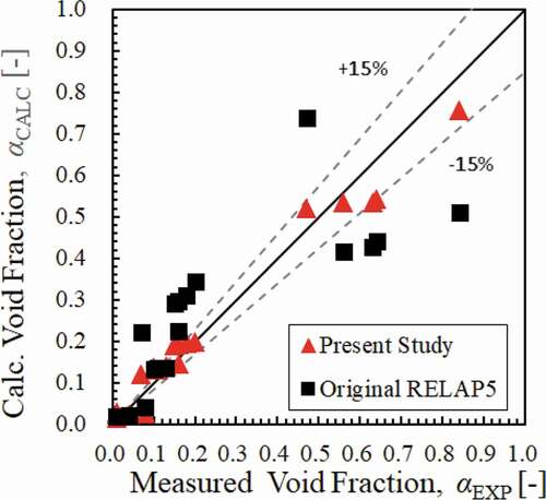
Calculated axial void fraction distributions for each condition are depicted in Figures 8–12. As can be seen from the figures, modified REAP5 calculation with newly developed drift–flux correlation predicts axial void fraction with better accuracy than the original RELAP5 output. The result suggests that utilizing accurate C_0,U correlation is crucial for the thermal-hydraulic analysis in nonuniformly distributed two-phase flows such as DOBO. Predictive capability of the RELAP5 void fraction values calculated using new C_0,U correlation with respect to the measurement is summarized in Figure 13. This result signifies that newly developed C_0,U correlations can be implemented into RELAP5 code without any issues and they are capable of calculating void fraction in DOBO within 15% of accuracy.

Figure 8. Axial void fraction development for the test condition R1.

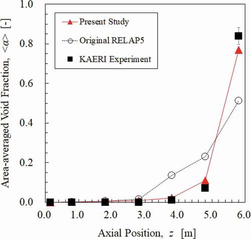
Figure 9. Axial void fraction development for the test condition R2.

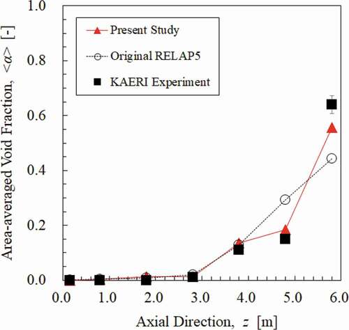
Figure 10. Axial void fraction development for the test condition R3.

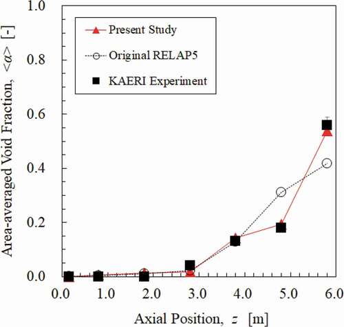
Figure 11. Axial void fraction development for the test condition R4.

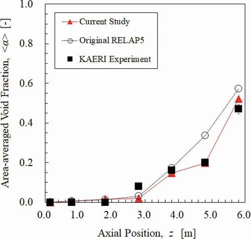
Figure 12. Axial void fraction development for the test condition R2-1a.

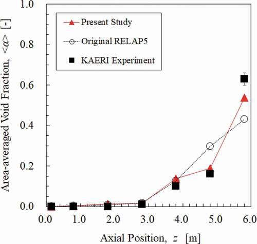
Figure 13. Performance evaluation of RELAP5 void fraction calculation.

5. Conclusion

Predictive capability of the void fraction in PWR downcomer section is crucial to ensure the core integrity for the accident analysis. Present study was conducted to improve the RELAP5 calculation for DOBO phenomenon. From the analytical approach, it was demonstrated that the distribution parameter value tends to be much larger than typical upward two-phase flow conditions when the recirculatory flow pattern is observed. The new distribution parameter correlations which can be applied to nonuniform two-phase flow pattern were developed from inverse analysis. Additionally, to simulate the recirculatory behavior in RELAP5 code, a new approach was proposed to separate upward two-phase flow and downward single-phase flow regions. Modified distribution correlations were implemented into RELAP5/MOD3.2 code, with Hibiki and Ishii’s drift velocity correlations. The calculated void fraction results showed that they are comparable to the experimental data obtained by KAERI within 15%.

The distribution parameter formulation developed in the current study is applicable only for the upward flow region in the downcomer channel, when it is splitted into 9:1 ratio for upward and downward flow. Since the DOBO experiment was designed as the scaled-down version of AP1000 prototype, the distribution parameter model in the current study can be applied for the safety analysis of AP1000. On the other hand, for the case of plants with ECCS injection system without DVI, different downcomer flow pattern is expected from the DOBO experiment. Hence, applicability of the channel split ratio of 9:1 as well as the distribution parameter correlation for upward flow region should be reexamined. However, the analysis approach introduced in the current study can not only be applicable for DOBO analysis, but for any type of flow patterns with one-side heated two-phase flow conditions using one-dimensional code analysis.

Nomenclature

Table

Ci	Drag coefficient
C0	Distribution parameter
D	Channel diameter
$D^{\ast }$	Hydraulic diameter-dependent Bond number
G	Mass flux
g	Gravitational acceleration
j	Mixture volumetric flux
$j_g$	Superficial gas velocity
$j_f$	Superficial liquid velocity
$j_f^{\ast }$	Nondimensional superficial liquid velocity
L	Upflow channel width
m	Constant for volumetric flow profile
n	Constant for void fraction profile
$p$	Pressure
$q^{\prime \prime }$	Heat flux
TECC	ECC temperature
$\mathit{v}$	Velocity
$V_{gj}$	Drift velocity
${\mathit{v}}_r$	Relative velocity
${\mathit{v}}_{r\mathrm{\infty }}$	Relative velocity between single gas particle and liquid phase
WECC	ECC mass flow rate
x	Radial position of flow channel
x0	Peak total superficial velocity location
Greek symbol
$\alpha$	Void fraction
${\alpha }_w$	Near wall void fraction
σ	Surface tension
$\rho$	Density
$\mathrm{\Delta }\rho$	Density difference between two phases
$\mu$	Dynamic viscosity
Subscripts
f	Liquid phase
g	Gas phase
i	Value at interface
m	Mixture
max	Maximum value
Mathematical symbol
< >	Area averaged quantity
≪ ≫	Void-weighted area averaged quantity

Disclosure statement

No potential conflict of interest was reported by the authors.

Correction Statement

This article has been republished with minor changes. These changes do not impact the academic content of the article.

Appendix

Here, step-by-step derivation of $⟨\alpha j⟩$_U for calculating C_0,U is shown. According to the downcomer schematic shown in Figure 4, $⟨\alpha j⟩$_U can be defined as follows:

(A1) $⟨\alpha j{⟩}_U=\frac{1}{L}\underset{0}{\overset{L}{\int }}\alpha jdx=\frac{1}{L}\underset{0}{\overset{x_0}{\int }}\alpha jdx+\frac{1}{L}\underset{x_0}{\overset{L}{\int }}\alpha jdx$(A1)

The integral of the first term on the right-hand side can be calculated as follows:

(A2) $\frac{1}{L}\underset{0}{\overset{x_0}{\int }}\alpha jdx=\frac{{\alpha }_W{j}_0}{L{x}_0}\underset{0}{\overset{x_0}{\int }}{\left(1-\frac{x}{L}\right)}^{n}xdx$(A2)

Conducting integration by substitution using variables defined below:

(A3) $X=1-\frac{x}{L},dX=-\frac{dx}{L},\frac{x:0\to x_0}{X:1\to X_0},X_0=1-\frac{x_0}{L}$(A3)

Equation (A2)(A2) $\frac{1}{L}\underset{0}{\overset{x_0}{\int }}\alpha jdx=\frac{{\alpha }_W{j}_0}{L{x}_0}\underset{0}{\overset{x_0}{\int }}{\left(1-\frac{x}{L}\right)}^{n}xdx$(A2) can be written as follows:

(A4) $\begin{array}{rl}& \frac{{\alpha }_W{j}_0}{L{x}_0}\underset{0}{\overset{x_0}{\int }}{\left(1-\frac{x}{L}\right)}^{n}xdx=\frac{{\alpha }_W{j}_0}{x_0}L\underset{X_0}{\overset{1}{\int }}{X}^n\left(1-X\right)dX\\ & =\frac{{\alpha }_W{j}_0}{x_0}L\underset{X_0}{\overset{1}{\int }}\left(X^n-X^{n+1}\right)dX\\ & =\frac{{\alpha }_W{j}_0}{x_0}L{\left[\frac{X^{n+1}}{n+1}-\frac{X^{n+2}}{n+2}\right]}_{X_0}^1\\ & =\frac{{\alpha }_W{j}_{0}L}{x_0}\left\{\frac{1}{n+1}-\frac{1}{n+2}-\frac{X_0^{n+1}}{n+1}+\frac{X_0^{n+2}}{n+2}\right\}\end{array}$(A4)

Likewise, the second term on the right-hand side of Equation (A1)(A1) $⟨\alpha j{⟩}_U=\frac{1}{L}\underset{0}{\overset{L}{\int }}\alpha jdx=\frac{1}{L}\underset{0}{\overset{x_0}{\int }}\alpha jdx+\frac{1}{L}\underset{x_0}{\overset{L}{\int }}\alpha jdx$(A1) can be expressed as

(A5) $\frac{1}{L}\underset{x_0}{\overset{L}{\int }}\alpha jdx=\frac{{\alpha }_W{j}_0}{L}\underset{x_0}{\overset{L}{\int }}{\left(1-\frac{x}{L}\right)}^n{\left(1-\frac{x-x_0}{L-x_0}\right)}^{m}dx=\frac{{\alpha }_W{j}_0}{L}\underset{x_0}{\overset{L}{\int }}{\left(\frac{L-x}{L}\right)}^n{\left(\frac{L-x}{L-x_0}\right)}^{m}dx=\frac{{\alpha }_W{j}_0}{L^{n+1}{\left(L-x_0\right)}^m}\underset{x_0}{\overset{L}{\int }}{\left(L-x\right)}^{n+m}dx$(A5)

To solve Equation (A5)(A5) $\frac{1}{L}\underset{x_0}{\overset{L}{\int }}\alpha jdx=\frac{{\alpha }_W{j}_0}{L}\underset{x_0}{\overset{L}{\int }}{\left(1-\frac{x}{L}\right)}^n{\left(1-\frac{x-x_0}{L-x_0}\right)}^{m}dx=\frac{{\alpha }_W{j}_0}{L}\underset{x_0}{\overset{L}{\int }}{\left(\frac{L-x}{L}\right)}^n{\left(\frac{L-x}{L-x_0}\right)}^{m}dx=\frac{{\alpha }_W{j}_0}{L^{n+1}{\left(L-x_0\right)}^m}\underset{x_0}{\overset{L}{\int }}{\left(L-x\right)}^{n+m}dx$(A5) with integration by substitution, variables are defined as follows:

(A6) $X=L-x,dX=-dx,\frac{x:x_0\to L}{X:\left(L-x_0\right)\to 0}$(A6)

The solution of Equation (A5)(A5) $\frac{1}{L}\underset{x_0}{\overset{L}{\int }}\alpha jdx=\frac{{\alpha }_W{j}_0}{L}\underset{x_0}{\overset{L}{\int }}{\left(1-\frac{x}{L}\right)}^n{\left(1-\frac{x-x_0}{L-x_0}\right)}^{m}dx=\frac{{\alpha }_W{j}_0}{L}\underset{x_0}{\overset{L}{\int }}{\left(\frac{L-x}{L}\right)}^n{\left(\frac{L-x}{L-x_0}\right)}^{m}dx=\frac{{\alpha }_W{j}_0}{L^{n+1}{\left(L-x_0\right)}^m}\underset{x_0}{\overset{L}{\int }}{\left(L-x\right)}^{n+m}dx$(A5) can be then obtained as follows:

(A7) $\underset{x_0}{\overset{L}{\int }}{\left(L-x\right)}^{n+m}dx=\underset{0}{\overset{L-x_0}{\int }}{X}^{n+m}dX={\left[\frac{X^{n+m+1}}{n+m+1}\right]}_0^{L-x_0}=\frac{{\left(L-x_0\right)}^{n+m+1}}{n+m+1}$(A7)

With Equation (A7)(A7) $\underset{x_0}{\overset{L}{\int }}{\left(L-x\right)}^{n+m}dx=\underset{0}{\overset{L-x_0}{\int }}{X}^{n+m}dX={\left[\frac{X^{n+m+1}}{n+m+1}\right]}_0^{L-x_0}=\frac{{\left(L-x_0\right)}^{n+m+1}}{n+m+1}$(A7) , integration for the second term of the right-hand side of Equation (A1)(A1) $⟨\alpha j{⟩}_U=\frac{1}{L}\underset{0}{\overset{L}{\int }}\alpha jdx=\frac{1}{L}\underset{0}{\overset{x_0}{\int }}\alpha jdx+\frac{1}{L}\underset{x_0}{\overset{L}{\int }}\alpha jdx$(A1) will eventually become,

(A8) $\begin{array}{rl}& \frac{1}{L}\underset{x{ }_0}{\overset{L}{\int }}\alpha jdx=\frac{{\alpha }_w{j}_0}{L^{n+1}{\left(L-x_0\right)}^m}\frac{{\left(L-x_0\right)}^{n+m+1}}{n+m+1}\\ & =\frac{{\alpha }_w{j}_0{\left(L-x_0\right)}^{n+1}}{\left(n+m+1\right)L^{n+1}}\\ & =\frac{{\alpha }_w{j}_0{\left(1-\frac{x_0}{L}\right)}^{n+1}}{\left(n+m+1\right)L^{n+1}}\end{array}$(A8)

Consequently, one can obtain the expression of $⟨\alpha j⟩$_U as follows:

(A9) $\begin{array}{rl}& ⟨\alpha j{⟩}_U=\frac{1}{L}\underset{0}{\overset{L}{\int }}\alpha jdx\\ & =\frac{{\alpha }_W{j}_{0}L}{x_0}\left\{\frac{1}{n+1}-\frac{1}{n+2}-\frac{{\left(1-\frac{x_0}{L}\right)}^{n+1}}{n+1}+\frac{{\left(1-\frac{x_0}{L}\right)}^{n+2}}{n+2}\right\}\\ & +\frac{{\alpha }_W{j}_0{\left(1-\frac{x_0}{L}\right)}^{n+1}}{n+m+1}\end{array}$(A9)

References

- The RELAP5 Development Team. REALP5/MOD3 Code manual volume IV models and correlations, NUREG/CR-5535, 1995, US Nuclear Regulatory Commission.
- Ozaki T, Hibiki T, et al. Effect of void fraction covariance on two-fluid model based code calculation in pip flow. Prog Nucl Energy. 2018;108:319–333.
- Ozaki T, Hibiki T, Miwa S, et al. Development of one-dimensional two-fluid model with consideration of void fraction covariance effect. J Nucl Sci Technol. 2018;55:575–598.
- Yun BJ, Euh DJ, Song CH. Downcomer boiling phenomena during the reflood phase of a large-break LOCA for the APR1400. Nucl Eng Design. 2008;238:2064–2074.
- Lee DW, No HC, Lee EH, et al. Experiment and RELAP5 analysis for the downcomer boiling of APR1400 under LBLOCA reflood phase”. Nucl Technol. 2006;153:175–183.
- Euh DJ, Huh BG, Yun BJ, Song CH and Kim IG. Performance evaluation of the safety analysis codes for subcooled boiling in a nuclear reactor downcomer during the late reflood phase of an LBLOCA. Nucl Technol. 2008;164:368–384.
- Ishii M. One-dimensional drift-flux model and constitutive equations for relative motion between phases in various two-phase flow regimes, Technical Report, ANL-77-47, 1997, Argonne National Laboratory, Argonne, IL, USA.
- Kataoka I, Ishii M. Drift flux model for large diameter pipe and new correlation for pool void fraction. Int J Heat Mass Transfer. 1987;30:1927–1939.
- Zuber N, Findlay JA. Average volumetric concentration in two-phase flow systems. J Heat Transfer. 1965;87:453–468.
- Hibiki T, Ishii M. One-dimensional drift-flux model for two-phase flow in a large diameter pipe. Int J Heat Mass Transfer. 2003;46:1773–1790.
- Hibiki T, Situ R Mi Y, et al. Modeling of bubble-layer thickness for formulation of one-dimensional interfacial area transport equation in subcooled boiling in two-phase flow. Int J Heat Mass Transfer. 2003;46:1409–1423.
Appendix
Here, step-by-step derivation of U for calculating C0,U is shown. According to the downcomer schematic shown in ,
U can be defined as follows: