Calculation of the ideal isochronous field for the SC200 cyclotron using the Nelder-Mead simplex algorithm

ABSTRACT

In this paper, we propose a numerical method for ideal isochronous field calculation for the SC200 isochronous cyclotron based on the Nelder-Mead simplex algorithm. In this method, the radial field distribution is represented by an nth-order polynomial, an objective function is defined to describe the relative error of the orbital frequency, and the ideal isochronous field is calculated by optimizing the coefficients of the polynomial to minimize the objective function using the Nelder-Mead simplex algorithm. A comparative analysis of the proposed method and conventional methods indicates that the proposed method provides a more accurate ideal isochronous field, especially in the vicinity of the extraction region where the field flutter is large.

KEYWORDS:

• Cyclotron
• isochronous field
• Nelder-Mead simplex method

1. Introduction

In recent years, many compact cyclotrons have been built for the purpose of ion therapy. The SC200 cyclotron is a superconducting proton cyclotron used for proton therapy; it can accelerate protons to 200 MeV [1]. SC200 has four spiral sectors; the mean magnetic field is approximately 2.95 T in the central region and 3.6 T in the extraction region, the extraction radius is approximately 60 cm, and the orbital frequency is 45.75 MHz. The details of the parameters of the SC200 cyclotron are listed in Table 1.

Table 1. Main parameters of the SC200 cyclotron

Parameters	Value
Average magnetic field (central/extraction)	2.95/3.64 T
Minimun/Maximun field	2.8/4.6 T
Number of sectors	4
Pole diameter	1.24 m
Extraction energy	200 MeV
Extraction radius	0.604 m
Maximum spiral angle	65°
Harmonic number	2
RF frequency	91.5 MHz

One of the factors that limit higher energy output in a classical cyclotron is the phase slip caused by the relativistic effect. In an isochronous cyclotron, the mean magnetic field (the azimuthally averaged component in the mid-plane) increases with the energy of the particles and maintains a constant orbital frequency to overcome the phase slip problem. The mean magnetic field that keeps the orbital frequency constant is called an ideal isochronous field.

As an analytical approximation to calculate the ideal isochronous field in cyclotrons, Gordon’s method has been proposed and applied for many years [2–4]. Gordon’s method is highly effective, with a small requirement of computational resources, and is highly accurate in the low-flutter area. However, it is well known that Gordon’s method cannot provide accurate results when the field flutter increases, because this method is based on the assumption that the equilibrium orbit of the particles deviates slightly from a circular orbit.

With the improvements in microcomputing performance in calculating speed and memory capacity, it has become possible to achieve a more accurate ideal isochronous field by a numerical calculation. In Ref [5]., a numerical method (the gyration frequency-based method) was proposed. The accuracy in the low-flutter area was greatly improved with this method; however, although the accuracy in the large-flutter area can meet the requirements of the physical design, it is still not very high and can be improved. In this study, we developed a numerical procedure that results in a comparatively higher accuracy for the calculation of the ideal isochronous field, especially in the vicinity of the extraction area where the flutter is large.

There are two steps in achieving field isochronism for the SC200 cyclotron. The ideal isochronous field calculation is the first step; after the ideal isochronous field has been determined, the shimming process is performed to realize the ideal isochronous field by adjusting the sector geometry or by trim coils [6–9]. Magnet shimming is commonly an iterative process, in which the real mean magnetic field is compared with the ideal isochronous field to evaluate the quality of the isochronism in each iteration, and the error between the ideal isochronous field and the real mean magnetic field encourages further shimming in the next iteration. Both the quality of the shimming process and the quality of the ideal isochronous field are important for the isochronism; the value of improving the ideal isochronous field is that it can guide the subsequent shimming processes and improve the isochronism for the SC200 cyclotron.

2. Calculation process

There are two input parameters for the isochronous field calculation. One is the flutter field, and the other is the required orbital frequency. Prior to the calculation, a previously calculated or measured 2D magnetic field map in the middle plane $B\left(r,\theta \right)$ should be given. The 2D magnetic field map $B\left(r,\theta \right)$ is composed of the mean field component $B_0\left(r\right)$ and the flutter field component $f\left(r,\theta \right)$:

(1) $B\left(r,\theta \right)=B_0\left(r\right)+f\left(r,\theta \right)$(1)

where

(2) $f\left(r,\theta \right)=\sum _{n=1,2,3\cdots }{A}_n\left(r\right)\cdot sinn\theta +B_n\left(r\right)\cdot cosn\theta$(2)

As an input parameter, the flutter field does not change in the calculation process; our algorithm searches for a suitable radial field distribution $B_0\left(r\right)$ that matches the flutter field $f\left(r,\theta \right)$ to let the orbital frequencies approach the required constant value along the equilibrium orbits. In order to improve the accuracy, one can also scale up and down the flutter field linearly according to the mean field value $B_0\left(r\right)$ for each radius. Choosing a constant flutter field or a variable flutter field does not affect the calculation process. We chose a constant flutter in our algorithm for convenience.

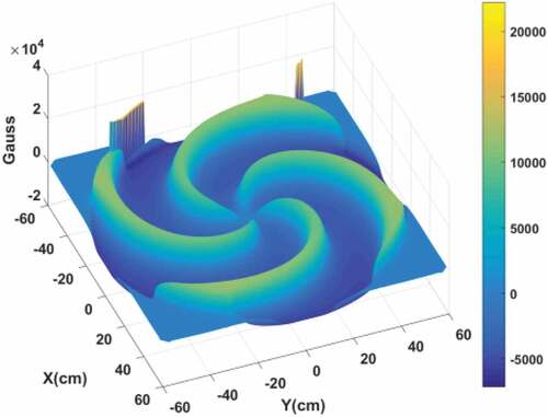
As an example, the previously calculated map of the magnetic field was derived from the SC200 cyclotron using a finite element method (FEM) simulation. The flutter field is shown in Figure 1. The required orbital frequency for the SC200 cyclotron is $f_0=45.75MHz$.

Figure 1. Overview of the flutter field of the SC200 cyclotron

The radial field distribution can be expanded into an nth-order polynomial:

(3) $B_{0i}\left(r\right)=a_0+a_1\cdot \left(r-r_{min}\right)+a_2\cdot {\left(r-r_{min}\right)}^2+\cdots +a_N\cdot {\left(r-r_{min}\right)}^N$(3)

For a given set of the coefficients $\left(a_0,a_1,a_2\cdots a_N\right)$, one can calculate the radial field distribution $B_{0i}\left(r\right)$ and then obtain the corresponding 2D field map $B_i\left(r,\theta \right)$. In each 2D field map, a number of equilibrium orbits are simulated to obtain the orbital frequency at different energies. Then, we define an objective function to describe the frequency error:

(4) $F\left\{B_{0i}\left(r\right)\right\}=\left|max\left(f_n-f_0\right)\right|$(4)

or equivalently,

(5) $F\left(a_0,a_1,\cdots ,a_N\right)=\left|max\left(f_n-f_0\right)\right|$(5)

where n denotes the energy steps, and $f_n=f\left(E_n\right)$ denotes the orbital frequency of the particles at energy $E_n$ for the given coefficients. It is evident that $F\ge 0$, and the objective function reaches a minimum (0) when the magnetic field $B_{0i}\left(r\right)$ is an ideal isochronous field. The magnitude of objective function values greater than the specified tolerance limit means that the magnetic field is different from the ideal isochronous field and hence it needs to be corrected by modifying the $a_N$ values. Therefore, the physical problem of determining the ideal isochronous field is transformed into the mathematical problem of finding the minimum value of the objective function $F\left(a_0,a_1,\cdots ,a_N\right)$; the Nelder-Mead simplex method is a simple and effective method for this optimization problem.

The Nelder-Mead simplex method, also called the simplex method, is a commonly used direct search method to minimize a function of multiple variables for which derivatives may not be known. This method uses the concept of a simplex, which is a special polytope of n + 1 vertices in n dimensions. Examples of simplexes include a line segment on a line, a triangle on a plane, a tetrahedron in three-dimensional space, and so forth. The simplex method in n dimensions (nth-order simplex method) maintains a set of n + 1 test points arranged as a simplex. Four possible operations (reflection, expansion, contraction, and shrink) are performed on the simplex according to the objective function values measured at each test point. A new simplex that has superior vertices will be formed in each iteration. Finally, the simplex can converge to the optimal solution after several iterations.

One can start with a set of arbitrary reasonable $a_N$ values and generate the initial simplex, but in order to improve the convergence speed, it is preferable to choose an initial simplex near the optimal solution; thus, we choose the mean field $B_{0g}\left(r\right)$ obtained from Gordon’s method and use the corresponding $a_N$ values to generate the first vertex and the initial simplex. Considering the coefficients $\left(a_0,a_1,a_2\cdots a_N\right)$as the first vertex of the initial simplex $X_0=\left(a_0,a_1,a_2,\cdots a_N\right)$, the other n vertexes of the initial simplex can be written

(6) $\left\{\begin{array}{c}{X}_1=\left(a_0,a_1+\mathrm{\Delta }{a}_1,a_2,\cdots ,a_N\right)\\ X_2=\left(a_0,a_1,a_2+\mathrm{\Delta }{a}_2,\cdots ,a_N\right)\\ \cdots \cdots \\ X_{\mathrm{N}}=\left(a_0,a_1,a_2\cdots ,a_N+\mathrm{\Delta }{a}_N\right)\end{array}\right.$(6)

in which the values of $\mathrm{\Delta }{a}_1,\mathrm{\Delta }{a}_2,\cdots ,\mathrm{\Delta }{a}_{\mathrm{N}}$ can be determined by

(7) $\mathrm{\Delta }{a}_i=\frac{\mathrm{\Delta }{B}_i}{{\left(r_{max}-r_{min}\right)}^i}$(7)

where $\mathrm{\Delta }{B}_i$ is the magnetic field error at the maximum radius. The selection of $\mathrm{\Delta }{B}_i$ is arbitrary; for example, $\mathrm{\Delta }{B}_1=4Gs$and $\mathrm{\Delta }{B}_2=5Gs$can be selected.

The iterative process of the simplex method has been described in many papers [10–12]. The iterative process starts from the initial simplex, and the N + 1 vertices of the initial simplex are ranked from lowest to highest function values. The vertex with the lowest function value is $X_l=\left(a_0,a_{l1},\cdots a_{lN}\right)$ (the best point), the vertex with the second-highest function value is $X_m=\left(a_0,a_{m1},\cdots a_{mN}\right)$ (the middle point), and the vertex with the highest function value is $X_h=\left(a_0,a_{h1},\cdots ,a_{hN}\right)$ (the worst point), which satisfies $F\left(X_l\right)<F\left(X_m\right)<F\left(X_h\right)$. Then, the centroids of all vertices excluding $X_h$ can be defined as

(8) $X_c=\frac{1}{n}\left[\sum _{i=0}^n{X}_i-X_h\right].$(8)

Generally, the optimal solution is in the opposite direction of $X_h$; the reflection point can be defined as $X_r$:

(9) $X_r=X_c+\alpha \left(X_c-X_h\right).$(9)

Usually, we select $1\le \alpha \le 1.5$, where $\alpha$ is the reflection coefficient. We calculate the value of the objective function $F\left(X_r\right)$ at $X_r$ and compare it with the function calculated at the other three points $X_l$, $X_m$, $X_h$, which results in four possible situations:

(1) The reflection point $X_r$ is better than the best point $X_l$:

$F\left(X_r\right)<F\left(X_l\right)<F\left(X_m\right)<F\left(X_h\right)$

(2) The reflection point $X_r$ is worse than the best point $X_l$ but better than the middle point $X_m$:

$F\left(X_l\right)<F\left(X_r\right)<F\left(X_m\right)<F\left(X_h\right)$

(3) The reflection point $X_r$ is worse than the middle point $X_m$ but better than the worst point $X_h$:

$F\left(X_l\right)<F\left(X_m\right)<F\left(X_r\right)<F\left(X_h\right)$

(4) The reflection point $X_r$ is worse than the worst point $X_h$:

$F\left(X_l\right)<F\left(X_m\right)<F\left(X_h\right)<F\left(X_r\right)$

Four possible operations (expansion, outside contraction, inside contraction, and shrink) are performed on the simplex according to each specific situation, and a new simplex that has superior vertices is obtained. The optimal solution can be obtained after several iterations. Finally, the isochronous mean field $B_0^{simp}\left(r\right)$ can be constructed by using the best vertex of the final simplex ${\vec{X}}_l$:

(10) $B_0^{simp}\left(r\right)=a_0+a_{l1}\cdot \left(r-r_{min}\right)+a_{l2}\cdot {\left(r-r_{min}\right)}^2+\cdots a_{lN}\cdot {\left(r-r_{min}\right)}^N$(10)

and the corresponding 2D field map in the mid-plane is reconstructed by adding the mean field component to the flutter field:

(11) $B_{simp}\left(r,\theta \right)=B_0^{simp}\left(r\right)+f\left(r,\theta \right)$(11)

The flow charts of the calculation process is shown in Figures 2 and 3.

Figure 2. Flow chart for the Nelder-Mead simplex method

Figure 3. Flow chart for calculating the objective function

To improve the calculation accuracy and speed, the entire computational domain can be divided into several small intervals; then, the isochronous field is calculated in each small interval in sequence. For example, the whole computational domain for the SC200 cyclotron is $R=10\sim 60.4cm$; we divided it into three small intervals, $R=10\sim 35cm$, $R=35\sim 50cm$, and $R=50\sim 60.4cm$. The first calculation is performed in the interval $R=10\sim 35cm$, the 2D field map obtained from the first calculation is further used as the input parameters for the second calculation in the interval $R=35\sim 50cm$, and so forth.

3. Comparison with traditional methods

To verify the performance of the proposed method, we compared it with Gordon’s method and the gyration frequency-based method. The 8^th-, 10^th-, and 12^th-order simplex methods, Gordon’s method, and the gyration frequency-based method were used to compute the ideal isochronous field under the same initial conditions.

A comparison of the results from Gordon’s method, the gyration frequency-based method, and the 12^th-order simplex method is shown in Figures 4–7, and a comparison of the accuracy and time cost using different-order simplex methods is shown in Figure 8.

Figure 4. Comparison of the isochronous field obtained from Gordon’s method, the gyration frequency-based method, and the 12^th-order simplex method

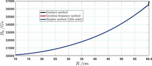
Figure 5. Difference between the isochronous field obtained from Gordon’s method, the gyration frequency-based method, and the 12^th-order simplex method

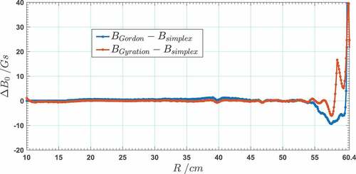
Figure 6. Relative error in the orbital frequency of Gordon’s method, the gyration frequency-based method, and the 12^th-order simplex method

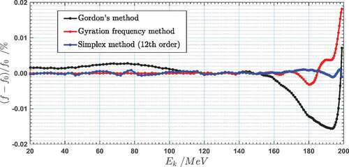
Figure 7. Comparison of the integrated phase slip during acceleration from 150 MeV to 200 MeV

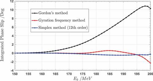
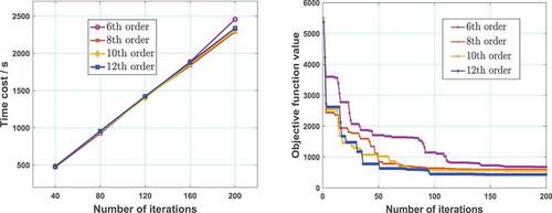
Figure 8. Time cost for different-order simplex methods (left), and the value of the objective function for different-order simplex methods during the iterations (right)

As seen in Figures 4 and 5, the results from the three methods are quite similar; the difference between the results from these three methods is nearly zero in the small-flutter area (R = 0–55 cm), but the difference increases to approximately 10–40 Gs in the large-flutter area (R = 55–60.4 cm). With the improvement of the 2D field measurement technique and shimming technique, the accuracy of the mean field can reach 10⁻⁴ in engineering; the correction provided by the proposed method is approximately 10⁻³ (40 Gs/36,000 Gs). Thus, the correction is quite large and should not be ignored, and this result can be useful for guiding the shimming process.

As shown in Figure 6, the relative error in the orbital frequency is small for all three methods in the interval of $E_k<150MeV$, but the error from Gordon’s method and the error from the gyration frequency-based method increase in the extraction region ($E_k>170MeV$) (approximately 0.0150%), whereas the error is quite small in the extraction region for the 12^th-order simplex method (approximately 0.0010%). As shown in Figure 7, the integrated phase slip is approximately 10° for Gordon’s method, approximately 2° for the gyration frequency-based method, and nearly 0° for the simplex method during acceleration from 150 MeV to 200 MeV (the energy gain is approximately 0.25 MeV per turn). Both of these results show substantial improvement in the field isochronism, which proves that the proposed method is highly useful in calculating the ideal isochronous field.

We also evaluated the performance of the proposed method by comparing the calculation speed for different-order simplex methods. We wrote MATLAB code for the ideal isochronous field calculation. This code runs on a workstation with 28 CPU cores using the parallel computing technique. The time cost and accuracy using different-order simplex methods are shown in Figure 8.

The calculation speed of the codes depends mainly on the efficiency of searching the equilibrium orbits. The order of the simplex methods has little effect on the calculation speed; a higher-order simplex method will not increase the time cost. In our example, the equilibrium orbits were calculated using Gordon’s procedure [13] with an azimuth step of 0.5°, the convergence accuracy of the equilibrium orbits is ${10}^{-6}m$. It takes approximately 1200 s to complete 100 iterations and 2400 s to complete 200 iterations. A lower objective function value suggests a more accurate isochronous field. The objective function value at the 200^th iteration decreases with an increase in the simplex order, which indicates that a higher-order simplex method improves the accuracy of the isochronous field calculation.

Because the proposed method must solve a large number of equilibrium orbits in the calculation process, it is computationally expensive, and the time cost is large. Although the computational efficiency is not high, the time cost is less than one hour with the help of the parallel computing technique, which is still acceptable; thus, this proposed method is effective for the ideal isochronous field calculation.

4. Application

The results of the proposed method can be applied in the shimming process. In general, magnet shimming is an iterative process containing two main steps: 1) qualify the isochronous error, and 2) predict the magnet pole shape modification according to the isochronous error.

In the first step, the ideal isochronous field can be used to evaluate the isochronous error:

(12) $\mathrm{\Delta }B\left(r\right)=B\left(r\right)-B_{iso}\left(r\right)$(12)

where $B\left(r\right)$ is the measured or calculated mean field, and $B_{iso}\left(r\right)$ is the ideal isochronous field given by the proposed method.

In the second step, the correlation matrix method [6, 8] is used to transform the isochronous error to pole geometry modification. In this method, we cut several rectangle patches from the pole edge at every radius to shim the isochronous field. The field change can be assumed to be the sum of the field change with every individual rectangle removed. The influence on the mean field of individual patches at radius $r=r_i$ is referenced as $a_i\left(r\right)$, which is pre-calculated in each radius with a radius step of $\mathrm{\Delta }r=1cm$ using the FEM simulation. Then, the field change is

(13) $\mathrm{\Delta }B\left(r\right)=\sum W_i\cdot a_i\left(r\right),$(13)

where $i$ denotes the radius steps, and $W_i$ is the width of the patch at $r_i$. The least-square method is employed to solve $W_i$, and then the pole geometry is adjusted in accordance with the $W_i$ values.

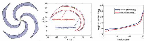
In the SC200 cyclotron, one degree of angle width is reserved on both sides of the pole for shimming; the structure of the SC200 poles and the angular width of the poles before and after shimming is shown in Figure 9.

Figure 9. Overview of the pole structure for SC200 (left), starting and optimized pole geometry (middle), and the angular width of the poles before and after shimming (right)

5. Summary

In this paper, we describe a numerical method for calculating the ideal isochronous field for the SC200 cyclotron. In this method, the radial field distribution is represented by an nth-order polynomial, an objective function is defined to describe the relative error of the orbital frequency, and the ideal isochronous field is calculated by optimizing the coefficients of the polynomial to minimize the objective function using the Nelder-Mead simplex algorithm.

The obtained result was compared with the isochronous fields computed by Gordon’s method and the gyration frequency-based method. The relative frequency error and the integrated phase slip were used as the field quality criteria. The relative error in the orbital frequency in the large-flutter area improved from 0.0150% to 0.0010%, and the integrated phase slip improved from 10° to nearly 0° by using the 12th-order simplex method for the SC200 cyclotron, which proves that the proposed method can yield a more accurate ideal isochronous field, especially in large-flutter areas such as the vicinity of the extraction radii.

The ideal isochronous field calculation is the first step in achieving isochronism for the SC200 cyclotron; after the ideal isochronous field is obtained, the real mean field is modified to approach the ideal isochronous field by adjusting the sector geometry in the shimming process. Both the quality of the ideal isochronous field and the quality of the shimming process are highly important for the isochronism.

The shimming technique has been greatly improved in recent years; however, the calculation of the ideal isochronous field is not commonly discussed. This paper presents an improvement in the ideal isochronous field calculation, which is helpful for improving the field isochronism for the SC200 cyclotron.

Acknowledgments

This work was supported by: (1) National Natural Science Foundation of China under [grant No. 11775258, 11575237], (2) International Scientific and Technological Cooperation Project of Anhui [grant No. 1704e1002207].

Disclosure statement

No potential conflict of interest was reported by the authors.

References

- Karamysheva G, Gurskiy S, Karamyshev O, et al. Compact superconducting cyclotron SC200 for proton therapy[C]. Proc Cyclotrons; Zurich, Switzerland; 2016.
- Tang JY, Wei BW. Theory and design of cyclotrons[M]. Hefei: University of Science and Technology of China Press; 2008.
- Gordon MM. Calculation of isochronous fields for sector-focused cyclotrons[J]. Part Accel. 1983;13:67–84.
- Gordon MM. Analysis of isochronous cyclotrons with separated hard-edge magnets[J]. Nucl Instrum Methods. 1970;83(2):267–271.
- Cirkovic S, Ristic-Djurovic JL, Ilic AZ, et al. Comparative analysis of methods for isochronous magnetic-field calculation[J]. IEEE Trans Nucl Sci. 2008;55(6):3531–3538.
- Qin B, Yang J, Liu KF. Precise isochronous field shimming using correlation matrix for compact cyclotrons[J]. Nucl Instrum Methods Phys Res A. 2012;691:129–134.
- Sing Babu P, Goswami A, Sarma PR, et al. Optimization of sector geometry of a compact cyclotron by random search and matrix methods[J]. Nucl Instrum Methods Phys Res A. 2010;624:560–566.
- Ming L, Zhong J, Cui T, et al. Application and development of a method to shim the isochronous field in small cyclotrons[J]. IEEE Trans Appl Supercond. 2013;26:4.
- Chen D, Liu K, Yang J, et al. Fast and accurate magnetic field shimming for a compact cyclotron[J]. IEEE Trans Nucl Sci. 2013;60(3):2175–2179.
- Wanga PC, Shoupb TE. Parameter sensitivity study of the Nelder–Mead simplex method[J]. Adv Eng Software. 2011;42(7):529–533.
- Gao F, Han. L. Implementing the Nelder-Mead simplex algorithm with adaptive parameters[J]. Comput Optim Appl. 2010;51(1):259–277.
- Han L, Neumann M. Effect of dimensionality on the Nelder-Mead simplex method[J]. Optim Methods Software. 2006;21(1):1–16.
- Gordon MM. Computation of closed orbits and basic focusing properties for sector-focused cyclotrons and the design of” cyclops”[J]. Part Accel. 1984;16:39–62.