Development of a reduced order model for severe accident analysis codes by singular value decomposition aiming probabilistic safety margin analysis

ABSTRACT

Severe accident codes (e.g. MAAP, RELAP, and MELCORE) model various physical phenomena during severe accidents. Many analyses using these codes for safety margin evaluation are impractical due to large computational costs. Surrogate models have an advantage of quickly reproducing multiple results with a low computational cost. In this study, we apply the singular value decomposition to the time-series results of a severe accident code to develop a reduced order modeling (ROM). Using the ROM, the probabilistic safety margin analysis for the station blackout with a total loss of feedwater capabilities at a boiling water reactor is carried out. The dominant parameters to the accident progression are assumed to be the down-time and the recovery-time of the reactor core isolation cooling system, and decay heat. To reduce the number of RELAP5/SCDAPSIM analyses while maintaining the prediction accuracy of ROM, we develop a data sampling method based on adaptive sampling, which selects the new sampling data based on the dissimilarity with the existing training data for ROM. Our ROM can rapidly reproduce the time-series results and can estimate core conditions. By reproducing multiple results by ROM, a time-dependent core damage probability distribution is calculated instead of the direct use of RELAP5/SCDAPSIM.

KEYWORDS:

• Singular value decomposition
• Reduced order modeling
• Adaptive sampling
• Severe accident code
• RELAP5/SCDAPSIM
• Safety margin analysis
• Station blackout

1. Introduction

After the severe accident (SA) at Fukushima Daiichi nuclear power plant in March 2011, the newly established Nuclear Regulation Authority (NRA) has developed the new regulatory standards for commercial nuclear reactor plants in July 2013 [1]. One of the key points in the new standards is the legal requirements for prevention and mitigation measures of SAs, which were voluntarily implemented by the utilities before the Fukushima Daiichi accident. Recently, some nuclear power plants, whose application has been approved by NRA, have started in Japan. In the future, each electric power company would consider the following in the view of safety and efficiency:

• Plant installation modifications.

• Additional safety measures for SAs.

• Plant life extension to 60 years.

• Improving operational efficiency using risk information and so on.

Utilities have strong motivation to quantify not only the frequency of SA (e.g. core damage frequency and CDF), but also actual safety margin distribution. Quantification of safety margin characteristics is called the risk-informed safety margin characterization (RISMC) [2]. For example, RISMC quantitatively evaluates the increased safety margin by accident management in accident scenarios. In reference [3], this evaluation is conducted by a large number of direct SA code analyses. However, such evaluation would be impractical for actual applications because it requires considerable longer calculation time (typically several hours for each analysis). Therefore, surrogate models, which quickly predict the results of SA analysis, have been proposed. The surrogate model methods are divided into two categories. The first one is the use of machine learning for the multiple results of an SA code. The proposed learning methods in the previous work were Gaussian Process Models (GPMs), K-Neighbors Regressor (KNR), Support Vector Regressor (SVR), Sheppard Interpolation Method, and Generalized Polynomial Chaos expansion (gPC) [4]. The previous study could reduce the computational cost of RISMC by using these surrogate models. However, these surrogate models were independently applied to each time-step of the time-series data. In other words, it requires many surrogate models to estimate a result with many time-steps. The second one is the use of an approximate physical model for SA progression. In the reference [5], the accident progression was estimated by a simple adiabatic and heat balance model; however, there are problems in this approach, i.e. the physical phenomena in SA progressions cannot be treated precisely and expertise is required in the choice of appropriate approximate models of the physical phenomena. The surrogate model developed in our study is classified as the former surrogate model using the results of an SA code.

In various accident scenarios, the time-series data have different characteristics. In a specific scenario, however, the time-series data often have similar behaviors; therefore, we consider the possibility that the time-series data can be reconstructed using the representative time-series vectors in a specific scenario. When the time-series data have lower similarity, the many representative vectors are necessary to cover various characteristics of the time-series data. Meanwhile, when the time-series data have higher similarity, the reconstruction accuracy will be high even with a smaller number of representative vectors. In our study, the singular value decomposition (SVD) is applied to extract representative vectors for ROM from the results of an SA code [6,7]. The basic idea of this approach is based on the study in the reference [8], in which a ROM for the time-series data of fission gas release rate in fuel performance modeling code Bison is constructed by the principal component analysis (PCA). PCA is a mathematical technique that decomposes a square matrix into an eigenvalue and an eigenvector, and SVD is regarded as an expansion from PCA into a non-square matrix. Because SVD can extract the dominant (representative) vectors of all time-series data, ROM can be constructed using the dominant vectors. In our study, the dominant vectors represent the trend of the time-series data calculated by an SA code. With the approach of our ROM using SVD, construction of ROM at each time-step is not necessary. Our ROM can reproduce the whole time-series data regardless of the number of time-steps in a scenario. The proposed method also has an advantage for the construction of ROM, as the choice of a learning model for physical phenomena and the optimization of hyperparameters are not necessary. The use of an approximate physical model requires a careful choice of an appropriate calculation model for physical phenomena to maintain the prediction accuracy; however, our ROM can be constructed using the results of an SA code, and can thus model various physical phenomena without a difficult choice of calculation models. The prediction accuracy of the machine-learning generally depends on the hyperparameters, which are tuned by the users. Such tuning by the users is however not desirable from the viewpoint of usability. Our ROM is easily constructed while maintaining accuracy because it does not require the optimization of hyperparameters. By using SVD, our study aims to develop a ROM for an SA code and to perform a probabilistic safety margin analysis by the constructed ROM.

The new contribution of this paper is the following three points. Firstly, we develop a new ROM using SVD for the results of an SA code to reduce computational cost. Our ROM can reproduce whole time-series data because it is constructed by representative time-series vectors extracted from the results of an SA code. Secondly, we introduce the concept of the gravity field into the adaptive sampling method [9]. The gravity field method gives the priority to select new sampling data based on the dissimilarity with the existing training data for ROM. The data sampling method based on adaptive sampling reduces the number of training data for ROM construction while maintaining the prediction accuracy of ROM. We also develop the convergence criterion for the data sampling method to avoid producing extra training data, which does not contribute to the improvement of prediction accuracy of ROM. Thirdly, we apply the ROM, which is constructed by SVD through the data sampling method based on the adaptive sampling, to a probabilistic safety margin analysis. In this study, the time-dependent core damage probability (CDP) distribution for station blackout (SBO) scenario is estimated by our ROM.

The rest of the study is organized as follows. The theoretical description, procedure, data sampling, and limitations of ROM construction are given in Section 2. Calculation conditions in this study and verification results of ROM for SBO with a total loss of feedwater capabilities are provided in Section 3. Finally, concluding remarks are summarized in Section 4.

2. Theory

2.1. Overview of ROM construction method

In this section, the overview of ROM construction is described. There are three key points in our developed ROM, i.e. SVD, the low-rank-approximation (LRA), and a data sampling method based on adaptive sampling.

In our study, the theory of our ROM is based on SVD, which extracts the dominant vectors that well express the trend of the matrix of many time-series data (Section 2.2.1). Considering the contribution ratio of vectors, LRA is applied to remove the minor vectors that have a small effect on the ROM results (Section 2.2.2). Finally, our ROM is constructed using the representative vectors and its expansion coefficients generated by SVD and LRA (Section 2.2.3). In the ROM that we have studied, the linear interpolation method is used for expansion coefficients corresponding to representative vectors extracted by SVD. The linear interpolation has three advantages: (1) avoidance of over-learning or over-fitting, (2) affinity with the present data sampling method, and (3) simplicity (Section 2.2.4).

To improve the prediction accuracy of ROM, the number of training data, i.e. the results by an SA code is generally increased. Because the computational cost of an SA code is usually high, a smaller number of training data is desirable to construct ROM. A data sampling method based on adaptive sampling is therefore applied to generate the training data that is expected to most improve the prediction accuracy of ROM while reducing extra computational cost. In the data sampling method based on adaptive sampling, our study newly introduces the concept of gravity field and convergence criterion (Section 2.3).

Finally, the proposed ROM assumes limitations to realize higher prediction accuracy. These limitations are described in Section 2.4.1. The time-series data are preprocessed to make the interval and the number of time-steps among different time-series data consistent for ROM construction with SVD. The approaches to align the interval and the number of time-steps are described in Section 2.4.2.

2.2. Theory of ROM construction

2.2.1. SVD

The SVD is a matrix operation to decompose any matrix to a diagonal matrix and orthogonal matrices [10]. The feature of SVD is to extract representative vectors, which express the trend of the original matrix. This section briefly describes the mathematical interpretation of SVD.

Using square matrices $\mathbf{U}=\left({\vec{u}}_1,{\vec{u}}_2,\dots {\vec{u}}_m\right)$ and ${\hspace{0.17em}}_{\hspace{0.17em}}^{\mathrm{T}}\mathbf{V}={\hspace{0.17em}}_{\hspace{0.17em}}^{\mathrm{T}}\left({\vec{v}}_1,{\vec{v}}_2,\dots {\vec{v}}_t\right)$, an $m\times t$ Hermitian matrix $\mathbf{A}$ is transformed into an $m\times t$ diagonal matrix $\mathrm{\Sigma }$:

(1) ${\hspace{0.17em}}_{\hspace{0.17em}}^{\mathrm{T}}\mathbf{U}\mathbf{A}\mathbf{V}=\mathrm{\Sigma },$(1)

where the diagonal matrix $\mathrm{\Sigma }$ is expressed as

(2) $\mathrm{\Sigma }=\left(\begin{array}{cccccc}{\sigma }_1& 0& \cdots & \cdots & \cdots & 0\\ 0& {\sigma }_2& 0& \ddots & \ddots & ⋮\\ ⋮& ⋮& \ddots & \ddots & \ddots & ⋮\\ 0& \cdots & 0& {\sigma }_m& \cdots & 0\end{array}\right)\left(m<t\right).$(2)

The diagonal components are singular values that take positive and monotonically decreasing values, i.e. ${\sigma }_1>{\sigma }_2>\cdots >{\sigma }_i\ge 0$ ($1\le i\le m$). The number $m$ corresponds to the rank of matrix $\mathbf{A}$. This diagonalization operation can be regarded as an extension of the diagonalization of a square matrix into a non-square matrix.

Because the matrices $\mathbf{U}$ and $\mathbf{V}$ are unitary, Equation (1)(1) ${\hspace{0.17em}}_{\hspace{0.17em}}^{\mathrm{T}}\mathbf{U}\mathbf{A}\mathbf{V}=\mathrm{\Sigma },$(1) becomes

(3) $\begin{array}{rl}& \mathbf{U}{}^{\mathrm{T}}\mathbf{U}\mathbf{A}\mathbf{V}{}_{\hspace{0.17em}}^{\mathrm{T}}\mathbf{V}=\mathbf{U}\mathbf{\Sigma }{}_{\hspace{0.17em}}^{\mathrm{T}}\mathbf{V}\\ & \mathbf{U}{\mathbf{U}}^{-1}\mathbf{A}\mathbf{V}{\mathbf{V}}^{-1}=\mathbf{U}\mathbf{\Sigma }{}_{\hspace{0.17em}}^{\mathrm{T}}\mathbf{V}\\ & \mathbf{E}\mathbf{A}\mathbf{E}=\mathbf{U}\mathbf{\Sigma }{}_{\hspace{0.17em}}^{\mathrm{T}}\mathbf{V}\\ & \mathbf{A}=\mathbf{U}\mathbf{\Sigma }{}_{\hspace{0.17em}}^{\mathrm{T}}\mathbf{V},\end{array}$(3)

where $\mathbf{U}$, $\mathbf{\Sigma }$, and $\mathbf{V}$ contain the left singular vectors, the singular values, and the right singular vectors, respectively. Note that ${\mathbf{U}}^{-1}={\hspace{0.17em}}_{\hspace{0.17em}}^{\mathbf{T}}\mathbf{U}$ for unitary matrix is used in the above derivation.

In general, singular values take positive and monotonically decreasing values. The right and left singular vectors are arranged in descending order of associate singular values. In other words, they are arranged in descending order from the viewpoint of the contribution ratio to the variance of matrices ${\hspace{0.17em}}_{\hspace{0.17em}}^{\mathrm{T}}\mathbf{A}\mathbf{A}$ and $\mathbf{A}{\hspace{0.17em}}_{\hspace{0.17em}}^{\mathrm{T}}\mathbf{A}$. The cumulative contribution ratio of singular vectors can be calculated by

(4) $\left(\mathrm{T}\mathrm{h}\mathrm{e}\mathrm{c}\mathrm{o}\mathrm{n}\mathrm{t}\mathrm{r}\mathrm{i}\mathrm{b}\mathrm{u}\mathrm{t}\mathrm{i}\mathrm{o}\mathrm{n}\mathrm{r}\mathrm{a}\mathrm{t}\mathrm{i}\mathrm{o}\mathrm{o}\mathrm{f}\mathrm{t}\mathrm{h}\mathrm{e}k-\mathrm{t}\mathrm{h}\mathrm{v}\mathrm{e}\mathrm{c}\mathrm{t}\mathrm{o}\mathrm{r}\right)=\frac{{{\sigma }_k}^2}{{\sum }_{i=1}^m{{\sigma }_i}^2},$(4)

$\left(\mathrm{T}\mathrm{h}\mathrm{e}\mathrm{c}\mathrm{u}\mathrm{m}\mathrm{u}\mathrm{l}\mathrm{a}\mathrm{t}\mathrm{i}\mathrm{v}\mathrm{e}\mathrm{c}\mathrm{o}\mathrm{n}\mathrm{t}\mathrm{r}\mathrm{i}\mathrm{b}\mathrm{u}\mathrm{t}\mathrm{i}\mathrm{o}\mathrm{n}\mathrm{r}\mathrm{a}\mathrm{t}\mathrm{i}\mathrm{o}\mathrm{o}\mathrm{f}\mathrm{t}\mathrm{h}\mathrm{e}{1}^{\mathrm{s}\mathrm{t}}\mathrm{t}\mathrm{o}k-\mathrm{t}\mathrm{h}\mathrm{v}\mathrm{e}\mathrm{c}\mathrm{t}\mathrm{o}\mathrm{r}\mathrm{s}\right)=\frac{{\sum }_{i=1}^k{{\sigma }_i}^2}{{\sum }_{i=1}^m{{\sigma }_i}^2}.(5)$

For example, if the cumulative contribution ratio up to the $k$-th vector is 0.99, the 1^st to $k$-th right singular vectors can cover 99% variance of the matrix ${\hspace{0.17em}}_{\hspace{0.17em}}^{\mathrm{T}}\mathbf{A}\mathbf{A}$, which means these vectors almost capture the behavior of the row direction of the matrix A. In other words, the rest $m-k$ right singular vectors only cover 1% variance of the matrix ${\hspace{0.17em}}_{\hspace{0.17em}}^{\mathrm{T}}\mathbf{A}\mathbf{A}$. This property also holds true in the case of $m\ge t$.

Let us consider a matrix A which is arranged by ${\vec{a}}_n$ ($1\le n\le m$) in the row direction.

(6) $\mathbf{A}=\left(\begin{array}{c}{\vec{a}}_1\\ {\vec{a}}_2\\ ⋮\\ {\vec{a}}_m\end{array}\right),$(6)

where ${\vec{a}}_n$ is a row vector with $t$ elements and there is no identical ${\vec{a}}_n$. The matrix A can be expanded as Equation (7)(7) $\left(\begin{array}{c}{\vec{a}}_1\\ {\vec{a}}_2\\ ⋮\\ {\vec{a}}_m\end{array}\right)=\mathbf{U}\mathbf{\Sigma }{\hspace{0.17em}}_{\hspace{0.17em}}^{\mathrm{T}}\mathbf{V}=\left({\vec{u}}_1,{\vec{u}}_2,\dots {\vec{u}}_m\right)\left(\begin{array}{cccccc}{\sigma }_1& 0& \cdots & \cdots & \cdots & 0\\ 0& {\sigma }_2& 0& \ddots & \ddots & ⋮\\ ⋮& ⋮& \ddots & \ddots & \ddots & ⋮\\ 0& \cdots & 0& {\sigma }_m& \cdots & 0\end{array}\right)\left(\begin{array}{c}{\hspace{0.17em}}_{\hspace{0.17em}}^{\mathrm{T}}{\vec{v}}_1\\ {\hspace{0.17em}}_{\hspace{0.17em}}^{\mathrm{T}}{\vec{v}}_2\\ ⋮\\ {\hspace{0.17em}}_{\hspace{0.17em}}^{\mathrm{T}}{\vec{v}}_t\end{array}\right)=\left(\begin{array}{cccc}{u}_{11}& u_{12}& \cdots & u_{1m}\\ u_{21}& u_{22}& \cdots & u_{2m}\\ ⋮& ⋮& \ddots & ⋮\\ u_{m1}& u_{m2}& \cdots & u_{mm}\end{array}\right)\left(\begin{array}{c}{\sigma }_1{\hspace{0.17em}}_{\hspace{0.17em}}^{\mathrm{T}}{\vec{v}}_1\\ {\sigma }_2{\hspace{0.17em}}_{\hspace{0.17em}}^{\mathrm{T}}{\vec{v}}_2\\ ⋮\\ {\sigma }_m{\hspace{0.17em}}_{\hspace{0.17em}}^{\mathrm{T}}{\vec{v}}_m\end{array}\right)$(7) in correspondence with Equation (3)(3) $\begin{array}{rl}& \mathbf{U}{}^{\mathrm{T}}\mathbf{U}\mathbf{A}\mathbf{V}{}_{\hspace{0.17em}}^{\mathrm{T}}\mathbf{V}=\mathbf{U}\mathbf{\Sigma }{}_{\hspace{0.17em}}^{\mathrm{T}}\mathbf{V}\\ & \mathbf{U}{\mathbf{U}}^{-1}\mathbf{A}\mathbf{V}{\mathbf{V}}^{-1}=\mathbf{U}\mathbf{\Sigma }{}_{\hspace{0.17em}}^{\mathrm{T}}\mathbf{V}\\ & \mathbf{E}\mathbf{A}\mathbf{E}=\mathbf{U}\mathbf{\Sigma }{}_{\hspace{0.17em}}^{\mathrm{T}}\mathbf{V}\\ & \mathbf{A}=\mathbf{U}\mathbf{\Sigma }{}_{\hspace{0.17em}}^{\mathrm{T}}\mathbf{V},\end{array}$(3) :

(7) $\left(\begin{array}{c}{\vec{a}}_1\\ {\vec{a}}_2\\ ⋮\\ {\vec{a}}_m\end{array}\right)=\mathbf{U}\mathbf{\Sigma }{\hspace{0.17em}}_{\hspace{0.17em}}^{\mathrm{T}}\mathbf{V}=\left({\vec{u}}_1,{\vec{u}}_2,\dots {\vec{u}}_m\right)\left(\begin{array}{cccccc}{\sigma }_1& 0& \cdots & \cdots & \cdots & 0\\ 0& {\sigma }_2& 0& \ddots & \ddots & ⋮\\ ⋮& ⋮& \ddots & \ddots & \ddots & ⋮\\ 0& \cdots & 0& {\sigma }_m& \cdots & 0\end{array}\right)\left(\begin{array}{c}{\hspace{0.17em}}_{\hspace{0.17em}}^{\mathrm{T}}{\vec{v}}_1\\ {\hspace{0.17em}}_{\hspace{0.17em}}^{\mathrm{T}}{\vec{v}}_2\\ ⋮\\ {\hspace{0.17em}}_{\hspace{0.17em}}^{\mathrm{T}}{\vec{v}}_t\end{array}\right)=\left(\begin{array}{cccc}{u}_{11}& u_{12}& \cdots & u_{1m}\\ u_{21}& u_{22}& \cdots & u_{2m}\\ ⋮& ⋮& \ddots & ⋮\\ u_{m1}& u_{m2}& \cdots & u_{mm}\end{array}\right)\left(\begin{array}{c}{\sigma }_1{\hspace{0.17em}}_{\hspace{0.17em}}^{\mathrm{T}}{\vec{v}}_1\\ {\sigma }_2{\hspace{0.17em}}_{\hspace{0.17em}}^{\mathrm{T}}{\vec{v}}_2\\ ⋮\\ {\sigma }_m{\hspace{0.17em}}_{\hspace{0.17em}}^{\mathrm{T}}{\vec{v}}_m\end{array}\right)$(7)

Therefore, ${\vec{a}}_n$ is expressed by using the right singular vector as

(8) ${\vec{a}}_n=\sum _{i=1}^m{u}_{ni}{\sigma }_i{}_{\hspace{0.17em}}^{\mathrm{T}}{\vec{v}}_i$(8)

In other words, the common orthogonal vectors, which can express ${\vec{a}}_n$ with linear combinations, are extracted from the matrix A by SVD. This property becomes key in the construction of ROM.

2.2.2. LRA

The orthogonal vectors of the right and the left singular vectors are arranged in the descending order of the contribution ratio of the variance of matrices ${\hspace{0.17em}}_{\hspace{0.17em}}^{\mathrm{T}}\mathbf{A}\mathbf{A}$ and $\mathbf{A}{\hspace{0.17em}}_{\hspace{0.17em}}^{\mathrm{T}}\mathbf{A}$. Even if small singular values are neglected, the matrix A can be accurately reconstructed by the rest of singular vectors and singular values. This dimensional reduction is known as LRA. Assuming that the behavior of ${\vec{a}}_n$ can be almost reproduced by the first $k$ singular values ($k\le m$), ${\vec{a}}_n$ can be approximated as Equation (9)(9) ${\vec{a}}_n=\sum _{i=1}^m{u}_{ni}{\sigma }_i{}_{\hspace{0.17em}}^{\mathrm{T}}{\vec{v}}_i\approx \sum _{i=1}^k{u}_{ni}{\sigma }_i{}_{\hspace{0.17em}}^{\mathrm{T}}{\vec{v}}_i={{\vec{a}}_n}^{\prime }\left(k<<m\right),$(9) . A similar approximation can be applied in the case of $m\ge t$.

(9) ${\vec{a}}_n=\sum _{i=1}^m{u}_{ni}{\sigma }_i{}_{\hspace{0.17em}}^{\mathrm{T}}{\vec{v}}_i\approx \sum _{i=1}^k{u}_{ni}{\sigma }_i{}_{\hspace{0.17em}}^{\mathrm{T}}{\vec{v}}_i={{\vec{a}}_n}^{\prime }\left(k<<m\right),$(9)

where the reproduction ratio is calculated by Equation (5)$\left(\mathrm{T}\mathrm{h}\mathrm{e}\mathrm{c}\mathrm{u}\mathrm{m}\mathrm{u}\mathrm{l}\mathrm{a}\mathrm{t}\mathrm{i}\mathrm{v}\mathrm{e}\mathrm{c}\mathrm{o}\mathrm{n}\mathrm{t}\mathrm{r}\mathrm{i}\mathrm{b}\mathrm{u}\mathrm{t}\mathrm{i}\mathrm{o}\mathrm{n}\mathrm{r}\mathrm{a}\mathrm{t}\mathrm{i}\mathrm{o}\mathrm{o}\mathrm{f}\mathrm{t}\mathrm{h}\mathrm{e}{1}^{\mathrm{s}\mathrm{t}}\mathrm{t}\mathrm{o}k-\mathrm{t}\mathrm{h}\mathrm{v}\mathrm{e}\mathrm{c}\mathrm{t}\mathrm{o}\mathrm{r}\mathrm{s}\right)=\frac{{\sum }_{i=1}^k{{\sigma }_i}^2}{{\sum }_{i=1}^m{{\sigma }_i}^2}.(5)$. The contribution ratio of each right singular vector decreases as the singular value ${\sigma }_i$ decreases. The right singular vectors, which have a high contribution ratio (e.g. ${\vec{v}}_1$, ${\vec{v}}_2$, and ${\vec{v}}_3$), are therefore chosen as vectors for ROM. In other words, LRA reduces computational cost with minimum loss of reproduction accuracy by ROM. Meanwhile, the right singular vectors, which have a low contribution ratio, do not express the overall trend of the matrix A, but express the unique trend of each ${\vec{a}}_n$ (i.e. noises). In other words, LRA can eliminate noises in each data of the matrix A.

2.2.3. Application of SVD and LRA to SA analysis

In this section, the procedure of ROM construction from the results of an SA code using SVD and LRA is described. The ROM is constructed by the following procedures:

1. Sample input parameters and perform a calculation by an SA code. This procedure is repeated m times.

2. Construct the matrix A of Equation (10)(10) $\mathbf{A}=\left(\begin{array}{c}{\vec{a}}_1\\ {\vec{a}}_2\\ ⋮\\ {\vec{a}}_m\end{array}\right)=\left(\begin{array}{cccc}{a}_{11}& a_{12}& \cdots & a_{1t}\\ a_{21}& a_{22}& \cdots & \ddots \\ ⋮& ⋮& \ddots & \ddots \\ a_{m1}& a_{m2}& \cdots & a_{mt}\end{array}\right),$(10) using the m simulation results.

3. Apply LRA to the matrix A through SVD. The m simulation results are expanded by the orthogonal basis obtained by SVD (Equation (13)(13) ${\vec{a}}_n\approx \sum _{i=1}^k{u}_{ni}{\sigma }_i{\hspace{0.17em}}_{\hspace{0.17em}}^{\mathrm{T}}{\vec{v}}_i,$(13) ).

4. Each expansion coefficient ${\sigma }_i{\vec{u}}_i$ is represented by a function of input parameters using correlation among the expansion coefficient ${\sigma }_i{\vec{u}}_i$ and input parameters.

5. Estimate the expansion coefficients $u_{pi}{\sigma }_i$ for any input parameters ‘$p$’ using the functions obtained in Step 4.

6. Reconstruct time-series data of an SA code for any input parameters by the expansion coefficients obtained in Step 5 and the orthogonal basis in Equation (13)(13) ${\vec{a}}_n\approx \sum _{i=1}^k{u}_{ni}{\sigma }_i{\hspace{0.17em}}_{\hspace{0.17em}}^{\mathrm{T}}{\vec{v}}_i,$(13) .

Some details of the ROM construction using SVD are explained. An SA code considers many input parameters because it models various physical phenomena that occur in SA processes. At first, the perturbed input parameters (e.g. decay heat) for ROM are selected in an accident scenario. The accident progressions are repeatedly analyzed m times within the range of perturbed input parameters (Step 1 in the above procedures). In other words, the number of samples is m. The identical number of time-steps (it is defined as t) is used for all simulations. For example, the number of time-steps is 150 when the time-step size of 100 [s] is applied for a 15,000 [s] simulation. To align the number of time-steps in different simulations, the final state of time-series data is assumed to be maintained up to 15,000 [s] when the analysis of an SA code is terminated before 15,000 [s]. The calculated time-series results, which are the row vectors, are gathered and formed into an $m\times t$ matrix as shown in Equation (10)(10) $\mathbf{A}=\left(\begin{array}{c}{\vec{a}}_1\\ {\vec{a}}_2\\ ⋮\\ {\vec{a}}_m\end{array}\right)=\left(\begin{array}{cccc}{a}_{11}& a_{12}& \cdots & a_{1t}\\ a_{21}& a_{22}& \cdots & \ddots \\ ⋮& ⋮& \ddots & \ddots \\ a_{m1}& a_{m2}& \cdots & a_{mt}\end{array}\right),$(10) . In the following equation, the operation in the case of $m<t$ is described, but the case of $m\ge t$ can be considered in a similar way.

(10) $\mathbf{A}=\left(\begin{array}{c}{\vec{a}}_1\\ {\vec{a}}_2\\ ⋮\\ {\vec{a}}_m\end{array}\right)=\left(\begin{array}{cccc}{a}_{11}& a_{12}& \cdots & a_{1t}\\ a_{21}& a_{22}& \cdots & \ddots \\ ⋮& ⋮& \ddots & \ddots \\ a_{m1}& a_{m2}& \cdots & a_{mt}\end{array}\right),$(10)

where $a_{mt}$ is the output data at the $t$-th time-step in the $m$-th sample (Step 2 in the above procedures). The matrix A can be decomposed into three matrices with the SVD:

(11) $\mathbf{A}=\mathbf{U}\mathbf{\Sigma }{\hspace{0.17em}}_{\hspace{0.17em}}^{\mathrm{T}}\mathbf{V}=\left({\vec{u}}_1{\vec{u}}_2\cdots {\vec{u}}_m\right)\left(\begin{array}{cccccc}{\sigma }_1& 0& \cdots & \cdots & \cdots & 0\\ 0& {\sigma }_2& 0& \ddots & \ddots & ⋮\\ ⋮& ⋮& \ddots & \ddots & \ddots & ⋮\\ 0& \cdots & 0& {\sigma }_m& \cdots & 0\end{array}\right){\hspace{0.17em}}_{\hspace{0.17em}}^{\mathrm{T}}\left({\vec{v}}_1{\vec{v}}_2\cdots {\vec{v}}_t\right),$(11)

where the left singular vector is an $m\times m$ column orthogonal matrix $\mathbf{U}=\left({\vec{u}}_1,{\vec{u}}_2,\dots ,{\vec{u}}_m\right)$, the singular value is an $m\times t$ matrix, and the right singular vector is a $t\times t$ transpose row orthogonal matrix ${\hspace{0.17em}}^{\mathrm{T}}\mathbf{V}={\hspace{0.17em}}^{\mathrm{T}}\left({\vec{v}}_1,{\vec{v}}_2,\cdots ,{\vec{v}}_t\right)$. When the identical accident progressions do not exist in the $m$ simulations, the rank of the matrix A is $m$.

When the cumulative contribution ratio up to the $k$-th vector is sufficiently large to accurately reproduce the matrix A, the matrix $\mathbf{U}\mathbf{\Sigma }{\hspace{0.17em}}_{\hspace{0.17em}}^{\mathbf{T}}\mathbf{V}$ is approximated as ${\mathbf{U}}^{\prime }{\mathbf{\Sigma }}^{\prime }{\hspace{0.17em}}_{\hspace{0.17em}}^{\mathbf{T}}{\mathbf{V}}^{\prime }$ with LRA described in Section 2.2.2:

(12) $\mathbf{A}\approx \left({\vec{u}}_1,{\vec{u}}_2,\cdots ,{\vec{u}}_k\right)\left(\begin{array}{cccc}{\sigma }_1& 0& \cdots & 0\\ 0& {\sigma }_2& \cdots & ⋮\\ ⋮& ⋮& \ddots & ⋮\\ 0& \cdots & \cdots & {\sigma }_k\end{array}\right){\hspace{0.17em}}_{\hspace{0.17em}}^{\mathrm{T}}\left({\vec{v}}_1,{\vec{v}}_2,\cdots ,{\vec{v}}_k\right)={\mathbf{U}}^{\prime }{\mathbf{\Sigma }}^{\prime }{\hspace{0.17em}}_{\hspace{0.17em}}^{\mathrm{T}}{\mathbf{V}}^{\prime },$(12)

where the left singular vector is an $m\times k$ column orthogonal matrix ${\mathbf{U}}^{\prime }=\left({\vec{u}}_1,{\vec{u}}_2,\dots ,{\vec{u}}_k\right)$, the singular value is a $k\times \mathrm{k}$ matrix, and the right singular vector is a $k\times t$ transpose row orthogonal matrix ${\hspace{0.17em}}^{\mathrm{T}}{\mathbf{V}}^{\prime }={\hspace{0.17em}}^{\mathrm{T}}\left({\vec{v}}_1,{\vec{v}}_2,\cdots ,{\vec{v}}_k\right)$. The rank of the matrix A is regarded as $k$.

The right singular vector ${\hspace{0.17em}}_{\hspace{0.17em}}^{\mathrm{T}}{\mathbf{V}}^{\prime }$ is regarded as the set of orthogonal vectors for time-series data. The $n$-th simulation result ${\vec{a}}_n$ in the matrix A ($1\le n\le m$) can thus be approximately expanded by the orthogonal vectors as

(13) ${\vec{a}}_n\approx \sum _{i=1}^k{u}_{ni}{\sigma }_i{\hspace{0.17em}}_{\hspace{0.17em}}^{\mathrm{T}}{\vec{v}}_i,$(13)

where $u_{ni}{\sigma }_i$ is the expansion coefficient corresponding to the right singular vector of the $i$-th row ($1\le i\le k$). The expansion coefficient is calculated by the left singular vector and the singular value:

(14) ${\mathbf{U}}^{\prime }{\mathbf{\Sigma }}^{\prime }=\left({\sigma }_1{\vec{u}}_1,{\sigma }_2{\vec{u}}_2,\cdots ,{\sigma }_k{\vec{u}}_k\right)=\left(\begin{array}{cccc}{u}_{11}{\sigma }_1& u_{12}{\sigma }_2& \cdots & u_{1k}{\sigma }_k\\ u_{21}{\sigma }_1& u_{22}{\sigma }_2& \cdots & u_{2k}{\sigma }_k\\ ⋮& ⋮& \ddots & ⋮\\ u_{m1}{\sigma }_1& u_{m2}{\sigma }_2& \cdots & u_{mk}{\sigma }_k\end{array}\right),$(14)

where $u_{mk}{\sigma }_k$ is the expansion coefficient of the $k$-th right singular vector for the $m$-th sample. We can thus represent a simulation result by the orthogonal vectors (i.e. the right singular vectors) and the associate expansion coefficients (Step 3 in the above procedures). Because a simulation result depends on input parameters, we can expect a correlation among the input parameters and the expansion coefficient ${\sigma }_i{\vec{u}}_i$. For example, ${\sigma }_i{\vec{u}}_i$ can be expressed as a polynomial of perturbed input parameters used in an SA code (Step 4 in the above procedures). When ${\sigma }_i{\vec{u}}_i$ is expressed as a linear function, the expansion coefficient $u_{pi}{\sigma }_i$ corresponding to unknown ‘$p$’ input data is estimated as

(15) $u_{pi}{\sigma }_i=ap+b,$(15)

where $a$ and $b$ are constants (Step 5 in the above procedures). Using the correlation among input parameters and ${\sigma }_i{\vec{u}}_i$, we can estimate $u_{pi}{\sigma }_i$ for any input parameter. Once we know $u_{pi}{\sigma }_i$, a simulation result can be easily reconstructed by Equation (13)(13) ${\vec{a}}_n\approx \sum _{i=1}^k{u}_{ni}{\sigma }_i{\hspace{0.17em}}_{\hspace{0.17em}}^{\mathrm{T}}{\vec{v}}_i,$(13) (Step 6 in the above procedures).

2.2.4. Functionalization of expansion coefficients

In this section, the functionalization method of the expansion coefficient $u_{pi}{\sigma }_i$ corresponding to input parameters is described.

As discussed in Section 2.2.3, ${\sigma }_i{\vec{u}}_i$ can be expressed as a function of perturbed input parameters used in an SA code. There are many interpolation methods, e.g. polynomial interpolation, Kriging, and so on, for functionalization. The linear interpolation method is however used for the ROM construction in this study as the linear interpolation method can avoid over-fitting and can also avoid the choice of models or hyperparameters in other interpolation models. The method of linear interpolation on N-dimensional scattered data [11] is used in this study to interpolate the expansion coefficient $u_{pi}{\sigma }_i$. Before performing the interpolation, the normalization of each input parameter is carried out in our study. The value $x$ of each input parameter is normalized so that the maximum ($x_{max}$) and minimum ($x_{min}$) values correspond to 1 and 0, respectively:

(16) $x_{norm}=\frac{x-x_{min}}{x_{max}-x_{min}},$(16)

where $x_{norm}$ is the $x$ after normalization.

2.3. Data sampling method based on adaptive sampling for ROM construction

2.3.1. Outline of ROM construction with adaptive sampling

In this section, the concept of a data sampling method based on the adaptive sampling is described to reduce the number of SA analyses for ROM construction while maintaining the prediction accuracy of ROM. We develop the concept of gravity field and convergence criterion introduced into adaptive sampling. The overview of the data sampling method used in our study is illustrated in Figure 1. The parts enclosed by the bold solid line in Figure 1 indicate the contributions of our study.

Figure 1. Overview of the data sampling method based on adaptive sampling.

The purpose of ROM is a quick reproduction of the results of an SA code. In the construction of ROM, the minimization of the number of training data obtained by an SA code while maintaining the prediction accuracy of ROM is desirable, as an SA code requires longer computational time. To apply the ROM for the CDP distribution calculation, the boundary between core intact and core damage in the input parameter space (it is named as the CD boundary in this study) should be accurately captured by ROM. A data sampling method to sample training data at the vicinity of CD boundary is therefore desirable for ROM construction; however, the actual CD boundary is unknown at the beginning of ROM construction. ROM has the advantage of quickly reproducing the multiple simulation results. The approximate CD boundary is estimated using multiple reproductions by ROM (it is named as the CDROM boundary in this study). The CDROM boundary is used to sample training data instead of the actual CD boundary. By sampling training data on the CDROM boundary, the prediction accuracy of ROM will improve because the selected data is densely sampled around the CDROM boundary. This sampling method is classified as an adaptive sampling method.

There are many input data on the CDROM boundary, as many combinations of input data on the CDROM boundary exist in input parameter space. A selection method of input data on the CDROM boundary is therefore necessary. In the selection of input data, we would like to choose input data that effectively improves the prediction accuracy of ROM. In our study, the concept of gravity field is developed to select data based on the dissimilarity with the existing training data for ROM. In other words, the data having less similarity with the existing training data is selected in the gravity field method. The dissimilarity is measured by the ‘distance’ in input data space as described later.

The convergence criterion is necessary for the adaptive sampling method because it utilizes an iteration method to obtain the training data for ROM. In our study, the convergence criterion is developed by focusing on the improvement of CDR boundary during iterations based on the gravity field method.

2.3.2. Details of ROM construction with adaptive sampling

In this section, more detail explanations of the ROM construction in our study are provided.

The data sampling method based on the adaptive sampling in our study is explained as follows. As the simplest case, one input parameter for an SBO scenario is considered. There is the time-series data $\vec{y}$ [°C] of peak cladding temperature (PCT) as a function of the time $x$ [s], which is the duration of a total loss of water injection during the accident progression. The maximum temperature $y_{max}$ exists in $\vec{y}$. The $y_{max}$ becomes higher as $x$ becomes longer and vice versa. Let us consider $T_{CD}$ [°C], which is the criterion for core damage. An input parameter $x_{CD}$ satisfying $y_{max}=T_{CD}$ exists when the duration of the total loss of water injection is sufficiently long. The $x_{CD}$ corresponds to the input data on the CD boundary. When $x_{CD}$ is known, we can accurately predict core conditions: however, the rigorous $x_{CD}$ cannot be identified before performing multiple calculations of an SA code. Instead of $x_{CD}$, $x_{CD,ROM}$ on the CDROM boundary can be obtained, as we can quickly reproduce a large number of simulation results ${\vec{y}}_{ROM}$ by ROM. When $y_{max,ROM}$ in ${\vec{y}}_{ROM}$ equals $T_{CD}$, the input data is regarded as $x_{CD,ROM}$. In other words, $x_{CD,ROM}$ satisfies $y_{max,ROM}=T_{CD}$. After performing the calculation of an SA code on $x_{CD,ROM}$ by an SA code, the new $\vec{y}$ is added to the training data of ROM. The prediction accuracy of the CDROM boundary can be improved because $x_{CD,ROM}$ approaches the vicinity of CD boundary as the number of iterations increases. When ROM perfectly predicts the results of an SA code, $x_{CD,ROM}$ converges to the rigorous CD boundary. It is noted that the training data for our ROM are required to include core intact and damage results to estimate $x_{CD,ROM}$ by interpolation, as the accuracy of extrapolation is generally worse than interpolation. The above explanation is the basis of a data sampling method based on the adaptive sampling in our study.

The gravity field method, which gives the priority to select data from the CDROM boundary, is explained as follows. In the case of multiple input parameters, ${\vec{x}}_{CD,ROM}$ cannot be uniquely defined because many ${\vec{x}}_{CD,ROM}$ are on the CDROM boundary. A selection method is, therefore, necessary to choose the next sampling data (${{\vec{x}}_{CD,ROM}}^{\prime }$) from the CDROM boundary. In the selection of the next sampling data, we would like to choose training data that efficiently improves the prediction accuracy of ROM with the view of reducing the computational cost. Let us assume that there are two candidate data for the next sampling. The first data is very close (similar) to the existing training data for ROM while the second one is far (dissimilar) from the existing training data. Because the ROM is based on interpolation of the training data, the second one will be more suitable than the first one, as the small improvement is expected by the first data. The gravity field method directly reflects this concept. In the gravity field method, each data is assumed as a planet with the same mass. Each planet has its own gravity field. Similarly, the existing training data form a gravity field. If we put new data into the existing system, the new data will receive gravity force from the existing data. The gravity force is larger when the location of the data is closer to the existing data and vice versa. The gravity force represents the similarity or dissimilarity between the new data and existing data. If we have several candidates for the next sampling data, we can, therefore, choose sampling data whose gravity force is the smallest. It should be noted that the similarity or dissimilarity is represented by the ‘distance’ in the gravity field method; thus, the definition of distance is important. Its definition will be described later.

This selection based on the concept of gravity field is carried out as follows. Two-dimensional input parameters, $\vec{x}={\hspace{0.17em}}_{\hspace{0.17em}}^{\mathrm{T}}\left(x_1,x_2\right)$, are considered for simplicity.

1. The range of $x_1$, which is specified by the user, is discretized into n grid points. The number of grid points (n) becomes the number of candidates on the CDROM boundary.

2. In the grid point for $x_1$, the $x_2$ satisfying $y_{max,ROM}=T_{CD}$ is estimated using multiple predictions of ROM. This calculation is carried out for all grid points for $x_1$. Now we have n candidates for ${{\vec{x}}_{CD,ROM}}^{\prime }$ on the CDROM boundary as the next sampling.

3. The one ${{\vec{x}}_{CD,ROM}}^{\prime }$ is selected from the n candidates for ${{\vec{x}}_{CD,ROM}}^{\prime }$. To select the ${{\vec{x}}_{CD,ROM}}^{\prime }$, which is expected to most improve the prediction accuracy of ROM, the concept of gravity field method is introduced. Equation (17)(17) $V=\sum _{i=1}^N\frac{1}{||{\vec{r}}_{i,ROM}-\vec{x}{ }_{CD,{ROM}^{\prime }}|{|}_2},$(17) is used as the index for selection:

   (17) $V=\sum _{i=1}^N\frac{1}{||{\vec{r}}_{i,ROM}-\vec{x}{ }_{CD,{ROM}^{\prime }}|{|}_2},$(17)

• where ${\vec{r}}_{i,ROM}$ is the $i$-th input parameter previously used for ROM construction, and $N$ is the total number of the training data for ROM.

Equation (17)(17) $V=\sum _{i=1}^N\frac{1}{||{\vec{r}}_{i,ROM}-\vec{x}{ }_{CD,{ROM}^{\prime }}|{|}_2},$(17) indicates that the $V$ for ${{\vec{x}}_{CD,ROM}}^{\prime }$ is evaluated using the distance from each training data of ROM. When the evaluated value of $V$ is small, the ${{\vec{x}}_{CD,ROM}}^{\prime }$ is dissimilar from the existing training data for ROM construction in the view of the location, and vice versa. When the value of $V$ is large, the ${{\vec{x}}_{CD,ROM}}^{\prime }$ will have little new information. On the contrary, when the value of $V$ is small, ${{\vec{x}}_{CD,ROM}}^{\prime }$ have different characteristic from the existing training data for ROM; thus, the ${{\vec{x}}_{CD,ROM}}^{\prime }$ has sufficient new information and is expected to effectively improve the prediction accuracy of ROM. Therefore, the ${{\vec{x}}_{CD,ROM}}^{\prime }$ with the minimum $V$ is selected for the next sampling data. It is noted that the elements of input parameters in ${\vec{r}}_{i,ROM}$ and ${\vec{x}}_{CD,ROM}$ are normalized (Equation (16)(16) $x_{norm}=\frac{x-x_{min}}{x_{max}-x_{min}},$(16) ) when Equation (17)(17) $V=\sum _{i=1}^N\frac{1}{||{\vec{r}}_{i,ROM}-\vec{x}{ }_{CD,{ROM}^{\prime }}|{|}_2},$(17) is applied. The above explanation is our development of the adaptive data selecting method based on the gravity field method.

Finally, the convergence of the CDROM boundary in the data sampling method based on the adaptive sampling is explained as follows. To observe the convergence of the CDROM boundary, matrix $X_{CD,ROM}=\left({{\vec{x}}_{1,CD,ROM}}^{\prime },{{\vec{x}}_{2,CD,ROM}}^{\prime },\cdots ,{{\vec{x}}_{n,CD,ROM}}^{\prime }\right)$, which consists of the n candidates for ${{\vec{x}}_{CD,ROM}}^{\prime }$ in the gravity field method, is used. The numbers of rows and columns of the matrix $X_{CD,ROM}$ correspond to ‘the dimension of input parameters’ and ‘the number of candidates (${{\vec{x}}_{CD,ROM}}^{\prime }$); $n$,’ respectively. Equation (18)(18) ${\epsilon }_l=||X_{l,CD,ROM}-X_{l-1CD,ROM}|{|}_2/||X_{l-1,CD,ROM}|{|}_2\left(l>1\right),$(18) is used to evaluate the ${\epsilon }_l$ in each iteration, which is used for the determination of convergence:

(18) ${\epsilon }_l=||X_{l,CD,ROM}-X_{l-1CD,ROM}|{|}_2/||X_{l-1,CD,ROM}|{|}_2\left(l>1\right),$(18)

where the subscript l indicates the number of iterations. Equation (18)(18) ${\epsilon }_l=||X_{l,CD,ROM}-X_{l-1CD,ROM}|{|}_2/||X_{l-1,CD,ROM}|{|}_2\left(l>1\right),$(18) shows the change of CDROM boundary when the new ${{\vec{x}}_{CD,ROM}}^{\prime }$ is added to the training data of ROM. The value of ${\epsilon }_l$ converges to zero because ${{\vec{x}}_{CD,ROM}}^{\prime }$ in $X_{l,CD,ROM}$ is expected to approach the vicinity of ${\vec{x}}_{CD}$ as the number of iterations increases. The convergence of the algorithm can be judged by the value of ${\epsilon }_l$. The degree of convergence is controlled by the user, which is compared with ${\epsilon }_l$.

To sum up, our ROM is constructed with the data sampling method based on the adaptive sampling by the following procedures when the number of input parameters is $d$:

1. Specify the range of input parameters by the user and choose the minimum and maximum values for each parameter. Minimum and maximum values correspond to core intact and damage (damage and intact) conditions, respectively.

2. Perform calculations of an SA code for $2^d$ input data combining the maximum and minimum value of input parameters. For example, when three parameters are considered for ROM construction, the eight $\left(2^3\right)$ input data are simulated by an SA code.

3. Construct ROM using SVD for the $2^d$ time-series results of an SA code (Section 2.2.3).

4. Calculate the ${{\vec{x}}_{CD,ROM}}^{\prime }$ to satisfy $y_{max,ROM}=T_{CD}$.

5. Using Equation (17)(17) $V=\sum _{i=1}^N\frac{1}{||{\vec{r}}_{i,ROM}-\vec{x}{ }_{CD,{ROM}^{\prime }}|{|}_2},$(17) based on the concept of gravity field, calculate $V$ using ${{\vec{x}}_{CD,ROM}}^{\prime }$ in Step 4, and sample ${{\vec{x}}_{CD,ROM}}^{\prime }$ with the lowest $V$.

6. Calculate the ${{\vec{x}}_{CD,ROM}}^{\prime }$ by an SA code. Our ROM is updated by adding the ${{\vec{x}}_{CD,ROM}}^{\prime }$ and the calculation result as the training data.

7. Repeat the iteration from Step 4 to 6. Iterations are finished when the convergence criterion is satisfied (Equation (18)(18) ${\epsilon }_l=||X_{l,CD,ROM}-X_{l-1CD,ROM}|{|}_2/||X_{l-1,CD,ROM}|{|}_2\left(l>1\right),$(18) ).

2.4. Limitations of ROM with SVD

2.4.1. Assumptions of ROM with SVD

In this section, two assumptions of ROM with SVD to achieve high prediction accuracy are described. Firstly, a ROM with SVD can be used for a specific accident scenario. Many accident scenarios for a nuclear power plant contain various time-scales and show completely different behaviors. Because SVD extracts dominant vectors that represent a majority of the time-series data, simultaneous treatment of accident scenarios having a completely different time-scale and the behavior will be difficult. Secondly, the perturbation range for input data should not be very large, as the treatment of completely different time-series data by SVD is difficult. The above two assumptions are considered to achieve higher accuracy of ROM with SVD.

2.4.2. Application of SVD to simulations of SA code

In this section, the treatment of the time-series data with different intervals and the number of time-steps is described to apply SVD. For the application of SVD, the time-series data are required to have an identical interval and the number of time-steps. However, the interval of time-steps is not uniform nor fixed in an SA code due to automated time-step control to minimize the calculation cost. Furthermore, a simulation may be terminated before the expected calculation time due to numerical instability of a calculation. The intervals and the number of time-steps can thus be different even in the same accident scenario. To align the intervals and the number of time-steps, the following approaches are considered. For the interval of time-step, the specific time-step to edit output parameter is provided through input data. For the number of time-steps, the data in the last step of time-series data is assumed to be maintained up to the expected simulation time as described in Section 2.2.3. By applying the above treatment, the intervals and the number of time-steps are identical among simulation results and can thus be directly used for SVD. When the above treatments are not appropriate to the time-series data, different treatments should be considered, but these are future tasks.

3. Calculations

3.1. Calculation conditions

3.1.1. Accident scenario

The accident scenario used in this study is the SBO with a total loss of feedwater capabilities at a boiling water reactor (BWR). The accident scenario is illustrated in Figure 2.

Figure 2. Accident progression in SBO with a total loss of feedwater capabilities.

At 0 [s], loss of off-site power occurs and the reactor is successfully shut down by scram. The feedwater and the recirculation pumps are tripped, the turbine throttle valve and main steam isolation valve are rapidly closed. The startup of the diesel generators is in fail (i.e. SBO). The reactor core isolation cooling system (RCIC) continuously injects water to the core because the direct current (DC) is available. Total feedwater is however lost owing to the RCIC or the battery fault at the time of $T_{down}$. Therefore, the decay heat cannot be removed. The accident then becomes more serious because the core temperature increases owing to the effect of decay heat. At $T_{restart}$, RCIC restarts owing to repairing. The occurrence of core damage depends on $T_{restart}$. If $T_{restart}$ is too large, the accident scenario progresses and the PCT reaches the critical temperature (i.e. the run-away temperature, approximately 1200°C). If $T_{restart}$ is small, the PCT is kept low and the core is intact. In the above accident scenario, quantitative evaluation of $T_{restart}$ is very important to terminate the accident sequence.

In this scenario, $T_{down}$, $T_{restart}$, and $F_{\gamma }$, which is decay heat (relative value), are considered as the input parameters having higher importance for accident progression in our study. In general, the dominant input parameters should be identified through sensitivity analysis; however, because the purpose of this study is the verification of our ROM construction method, exhaustive sensitivity analyses for input parameters have not been carried out. Table 1 summarizes the range of $T_{down}$, $T_{restart}$, and $F_{\gamma }$ considered in our study. It is noted that T_restart in Table 1 is the subtracted value of T_down. In this study, the probability distributions of $T_{down}$ and $T_{restart}$ are assumed to be uniform because our study aims to verify the construction of ROM with SVD. The other distributions based on probabilistic risk analysis or human reliability analysis would be considered as realistic safety analysis. The uncertainty of decay heat is considered as obeying a normal distribution (relative standard deviation: $1\sigma =$10%) [12]. The range of $F_{\gamma }$ is thus set as 2$\sigma$ to include the true value of decay heat with approximately 95% probability.

Table 1. Uncertainties of the input parameter.

Input Parameter	Minimum	Maximum	Distribution
Down time of RCIC ($T_{down}$) [s]	600	1800	Uniform
Recovery time of RCIC ($T_{restart}$) [s]	900	7200	Uniform
Decay heat (relative value, $F_{\gamma }$) [-]	0.8	1.2	Gaussian

3.1.2. SA code and plant model

The RELAP5/SCDAPSIM code [13] is used in the SA analysis. The plant model for Lagna Verde Unit 1 and Unit 2 (rated power: 1931 MW), which is BWR-5 designed by General Electric company, is used.

3.1.3. Criterion of core damage

The output training data obtained by RELAP5/SCDAPSIM code is PCT. To judge core intact or damage, maximum PCT (MPCT), which is the maximum value reached during the entire course of the simulation, is focused. The MPCT of 1200°C has been used as the criterion for core damage, which is adopted in the Japanese ECCS safety assessment guideline for LWRs [14].

The ROM to predict PCT during the accident is constructed using the calculation results by RELAP5/SCDAPSIM. When MPCT exceeds 1200°C, the core is judged as damaged.

3.1.4. Setting of time-steps

In this study, the accident progression of 15,000 [s] is analyzed. The calculation results are then discretized into 150 time-steps while assuming that the time-step size to edit output is 100 [s]. Identical discretization is used for all RELAP5/SCDAPSIM calculation results.

In some cases, RELAP5/SCDAPSIM calculations terminated during execution due to the instability of the calculation. Such termination usually occurs at the water injection by RCIC to the heated core. In this case, the value of PCT at the terminated time-step is used for the successive time-steps as described in section 2.2.3 and section 2.4.2. This treatment would be appropriate because PCT usually decreases when RCIC starts water injection. Because MPCT during the accident is important in this study, this treatment would be justified.

3.2. Calculation procedures

3.2.1. ROM construction

In accordance with the ROM construction described in Section 2.2, the procedures of ROM construction, which estimate fuel cladding temperature with the perturbed input parameters $T_{down}$, $T_{restart}$, and $F_{\gamma }$ are summarized as follows.

1. Make eight ($2^3$) input files combining the maximum and minimum value of $T_{down}$, $T_{restart}$, and $F_{\gamma }$ in Table 1.

2. Perform RELAP5/SCDAPSIM calculations. In our study, $\left(T_{down},T_{restart},F_{\gamma }\right)=\left(1800\left[s\right],10000\left[s\right],0.8\left[-\right]\right)$ is added to the initial data for ROM, as the core is intact at $\left(T_{down},T_{restart},F_{\gamma }\right)=\left(1800\left[s\right],9000\left[s\right],0.8\left[-\right]\right)$.

3. Generate the matrix A of Equation (10)(10) $\mathbf{A}=\left(\begin{array}{c}{\vec{a}}_1\\ {\vec{a}}_2\\ ⋮\\ {\vec{a}}_m\end{array}\right)=\left(\begin{array}{cccc}{a}_{11}& a_{12}& \cdots & a_{1t}\\ a_{21}& a_{22}& \cdots & \ddots \\ ⋮& ⋮& \ddots & \ddots \\ a_{m1}& a_{m2}& \cdots & a_{mt}\end{array}\right),$(10) by the nine results of RELAP5/SCDAPSIM.

4. Construct ROM through SVD and LRA for the matrix A. Unless otherwise noted, the vectors for ROM were reduced to cover 99.99% variance of the matrix ${\hspace{0.17em}}_{\hspace{0.17em}}^{\mathrm{T}}\mathbf{A}\mathbf{A}$ (cumulative contribution ratio defined by Equation (5)$\left(\mathrm{T}\mathrm{h}\mathrm{e}\mathrm{c}\mathrm{u}\mathrm{m}\mathrm{u}\mathrm{l}\mathrm{a}\mathrm{t}\mathrm{i}\mathrm{v}\mathrm{e}\mathrm{c}\mathrm{o}\mathrm{n}\mathrm{t}\mathrm{r}\mathrm{i}\mathrm{b}\mathrm{u}\mathrm{t}\mathrm{i}\mathrm{o}\mathrm{n}\mathrm{r}\mathrm{a}\mathrm{t}\mathrm{i}\mathrm{o}\mathrm{o}\mathrm{f}\mathrm{t}\mathrm{h}\mathrm{e}{1}^{\mathrm{s}\mathrm{t}}\mathrm{t}\mathrm{o}k-\mathrm{t}\mathrm{h}\mathrm{v}\mathrm{e}\mathrm{c}\mathrm{t}\mathrm{o}\mathrm{r}\mathrm{s}\right)=\frac{{\sum }_{i=1}^k{{\sigma }_i}^2}{{\sum }_{i=1}^m{{\sigma }_i}^2}.(5)$).

5. Estimate the input parameters ${{\vec{x}}_{CD,ROM}}^{\prime }$ corresponding to MPCT=1200°C by ROM. The total number of ${{\vec{x}}_{CD,ROM}}^{\prime }$ is 961 because $T_{down}$ and $F_{\gamma }$ were both divided into 31 points in the range shown in Table 1 and $T_{restart}$ was predicted by ROM for each combination of $T_{down}$ and $F_{\gamma }$.

6. Select 12 points from 961 candidates for ${{\vec{x}}_{CD,ROM}}^{\prime }$. Equation (17)(17) $V=\sum _{i=1}^N\frac{1}{||{\vec{r}}_{i,ROM}-\vec{x}{ }_{CD,{ROM}^{\prime }}|{|}_2},$(17) is used to choose 12 points as follows. After the ${{\vec{x}}_{CD,ROM}}^{\prime }$ with minimum $V$ is chosen and added to the training data of ROM (${\vec{r}}_{i,ROM}$), the next ${{\vec{x}}_{CD,ROM}}^{\prime }$ with the minimum $V$, which is evaluated by Equation (17)(17) $V=\sum _{i=1}^N\frac{1}{||{\vec{r}}_{i,ROM}-\vec{x}{ }_{CD,{ROM}^{\prime }}|{|}_2},$(17) using the new ${\vec{r}}_{i,ROM}$, is chosen from the rest of the candidates for ${{\vec{x}}_{CD,ROM}}^{\prime }$. Repeat the procedure until the number of ${{\vec{x}}_{CD,ROM}}^{\prime }$ is 12. Note that 12 parallel calculations are carried out in this study.

7. Perform RELAP5/SCDAPSIM calculations on the 12 ${{\vec{x}}_{CD,ROM}}^{\prime }$.

8. The 12 results by RELAP5/SCDAPSIM are added to the training data for ROM. The total number of training data for ROM becomes 21 (9 + 12).

9. Repeat Steps from 4 to 8. The total number of training data in the l-th iteration becomes 9 + 12(l-1). In our study, 13 iterations are carried out.

3.2.2. Core damage probability distribution

The final purpose of our study using ROM is to reduce the computational cost in the probabilistic safety margin analysis. The calculation procedure of CDP distribution using ROM is described in this section.

In this study, the core condition depends on the three parameters, i.e. the down, restart time of RCIC, and decay heat: $\left(T_{down},T_{restart},F_{\gamma }\right)$. In general, CDP becomes higher when $T_{down}$ is shorter and/or $T_{restart}$ is longer. In this study, the CDP distribution considering the uncertainty of decay heat is calculated for various $T_{down}$ and $T_{restart}$ as follows:

1. Divide the range of $T_{down}$ and $T_{restart}$ shown in Table 1 into 13 and 50 grid points, respectively.

2. Perform 10,000 random samplings of $F_{\gamma }$ at each of 650 (13$\times$50) points while assuming normal distribution $\mathcal{N}\left(1.0,0.1\right)$. When the sampled value of $F_{\gamma }$ exceeds the range of $2\sigma \left(F_{\gamma }<0.8,F_{\gamma }>1.2\right)$, resampling is performed because the range of $F_{\gamma }$ covered by ROM is set as [0.8, 1.2].

3. ROM reproduces the 6.5 million (13$\times$50$\times$10,000) results instead of RELAP5/SCDAPSIM.

4. In each combination of $T_{down}$ and $T_{restart}$, the number of samples judged as the core damage is counted when the MPCT estimated by ROM exceeds 1200°C. When the numbers of the core damage cases and random sampling cases are p and N (10,000), respectively, the CDP is estimated as

   (19) $\mathrm{C}\mathrm{D}\mathrm{P}=\mathrm{p}/\mathrm{N},$(19)

where the uncertainty of CDP is estimated as

(20) ${\sigma }_{\mathrm{C}\mathrm{D}\mathrm{P}}=\sqrt{\mathrm{C}\mathrm{D}\mathrm{P}\cdot \left(1-\mathrm{C}\mathrm{D}\mathrm{P}\right)/\mathrm{N}}.$(20)

It is noted that ${\sigma }_{\mathrm{C}\mathrm{D}\mathrm{P}}$ in Equation (20)(20) ${\sigma }_{\mathrm{C}\mathrm{D}\mathrm{P}}=\sqrt{\mathrm{C}\mathrm{D}\mathrm{P}\cdot \left(1-\mathrm{C}\mathrm{D}\mathrm{P}\right)/\mathrm{N}}.$(20) only includes the statistical uncertainty and excludes the uncertainty propagated from the ROM construction.

3.3. Results and discussions

3.3.1. Construction result of ROM

Figures 3 and 4 show the initial input data for ROM and the time-series data of PCT obtained by RELAP5/SCDAPSIM calculations using initial data.

Figure 3. Input parameters to construct initial ROM.

Figure 4. Time-series data of peak cladding temperature calculated by RELAP5/SCDAPSIM used to construct initial ROM.

Using the data in Figures 3 and 4, the initial ROM was constructed. The three main vectors with a high contribution ratio in the right singular vector are shown in Figure 5.

Figure 5. Right singular vectors which represent over 99.34% variance of time-series data in initial ROM in Figure 4. The contribution ratio of each vector is shown in the legend.

These three vectors cover more than 99.34% variance of the training data in Figure 4.

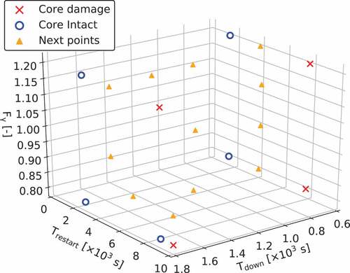
The ${{\vec{x}}_{CD,ROM}}^{\prime }$ (961 points) estimated by the initial ROM (the CDROM boundary), which are marked as triangles, are shown in Figure 6. The 12 points in ${{\vec{x}}_{CD,ROM}}^{\prime }$ for the next sampling are shown in Figure 7. These 12 points are chosen based on the procedure described in Section 2.3.2 and equally scattered in input space.

Figure 6. The candidates for ${{\vec{x}}_{CD,ROM}}^{\prime }$ on CDROM boundary at the initial iteration (triangular).

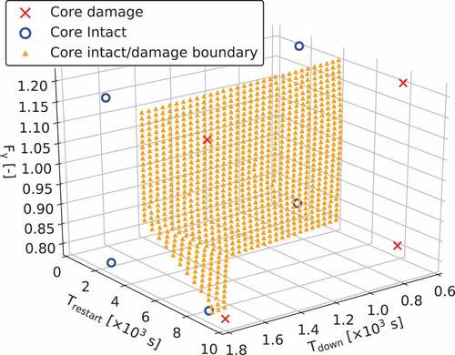
Figure 7. The next sampling points selected from ${{\vec{x}}_{CD,ROM}}^{\prime }$ at the initial iteration.

Figure 8 shows the input training data for ROM construction and the improvement of the CDROM boundary ${{\vec{x}}_{CD,ROM}}^{\prime }$ predicted by ROM up to the 13^th iteration.

Figure 8. The candidates for ${{\vec{x}}_{CD,ROM}}^{\prime }$ on CDROM boundary in the 2^nd, 5^th, 9^th, and 13^th iterations.

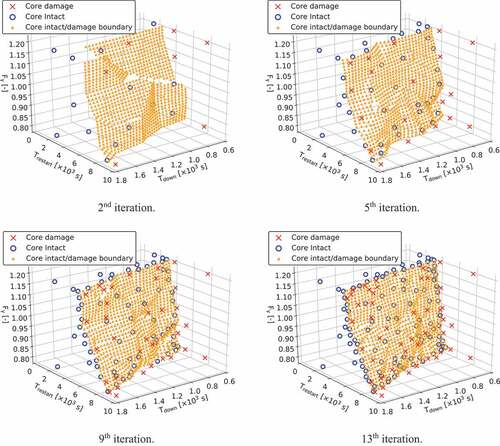
Figure 8 indicates that the input training data gathered in the vicinity of ${{\vec{x}}_{CD,ROM}}^{\prime }$ as the number of iteration increases. In other words, the output training data is sampled around MPCT = 1200°C.

Both the convergence and accuracy of the sampling method used in this study are shown in Figures 9 and 10, respectively.

Figure 9. The variation of ${\epsilon }_l$ in each iteration (the number of iterations; $l>1$).

Figure 10. The variation of mean absolute error calculated by leave-one-out cross-validation in each iteration.

From Figure 9, the ${\epsilon }_l$ indicates the convergence of the CDROM boundary estimated by ROM. At the beginning of the iteration, the CDROM boundary significantly changes when the new training data are added. The ${\epsilon }_l$ tends to decrease as the number of iterations increases, which means that the CDROM boundary converges to a certain surface. From Figure 10, the mean absolute error of MPCT, which is evaluated by leave-one-out cross-validation, tends to decrease as the number of iterations increases. In the 13^th iteration, ROM can estimate MPCT obtained by RELAP5/SCDAPSIM calculations with an average error of approximately $\left(1.06\pm 0.14\right)\times 100$°C. It is noted that the eight combinations of upper and lower $T_{down}$, $T_{restart}$, $F_{\gamma }$ are excluded in leave-one-out cross-validation because the interpolation is used. From the above, the validity of ROM construction by the sampling method used in this study is shown in the view of the convergence and accuracy of the algorithm.

3.3.2. Core damage probability distribution by ROM using SVD

The CDP distribution considering the uncertainty of decay heat is shown in Figure 11.

Figure 11. Core damage probability distribution for various $T_{down}$ and $T_{restart}$ estimated by multiple reproductions of ROM.

Increase of CDP as a function of $T_{restart}$ gradually becomes slower as $T_{down}$ becomes longer because heat decay decreases as a function of elapsed time after scram. This is the reason why CDP becomes lower as $T_{down}$ becomes longer. The CDP distribution shown in Figure 11 is consistent with physical insight.

The CDP calculated by ROM is compared with the CDP calculated by RELAP5/SCDAPSIM. Owing to the limitation of computational resources, four representative points are selected for verification and the accurate CDP was estimated by 1,000 calculations of RELAP5/SCDAPSIM in each point. The representative points are selected in the surrounding center and the edge of CDP distribution in Figure 11. The CDPs are shown in Table 2.

Table 2. Comparison of estimated core damage probability between ROM and RELAP5/SCDAPSIM. The number of samples is 10,000 for ROM and 1,000 for RELAP5/SCDAPSIM.

Input parameters		Core damage probability
$T_{down}$ [s]	$T_{restart}$ [s]	ROM	RELAP5/SCDAPSIM
900	4630	0.646 ± 0.005	0.51 ± 0.02
1200	5440	0.554 ± 0.005	0.50 ± 0.02
1500	6510	0.608 ± 0.005	0.68 ± 0.01
1800	6300	0.283 ± 0.005	0.12 ± 0.01

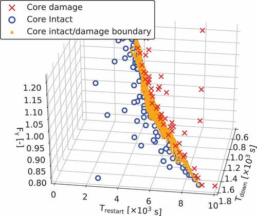
From Table 2, the CDPs by ROM roughly reproduce the CDPs calculated by RELAP5/SCDAPSIM within the error of approximately 16%. These results are caused by the difference in the CDROM boundary between ROM and RELAP5/SCDAPSIM. The limits of $F_{\gamma }$ on the CDROM boundary predicted by ROM and RELAP5/SCDAPSIM are compared in Figure 12 as a function of the number of iterations.

Figure 12. Comparison of the limit $F_{\gamma }$ on the CDROM boundary between ROM and RELAP5/SCDAPSIM in each iteration. If the limit $F_{\gamma }$ estimated by ROM is out of [0.8, 1.2], it is evaluated by using the value of $F_{\gamma }$ boundary.

From Figure 12, the limit $F_{\gamma }$ estimated by ROM approaches the limit $F_{\gamma }$ calculated by RELAP5/SCDAPSIM as the number of iterations increases. In the case of $\left(T_{down},T_{restart}\right)=\left(900\left[s\right],4630\left[s\right]\right)$ and $\left(1200\left[s\right],5440\left[s\right]\right)$, ROM can accurately estimate the limit $F_{\gamma }$ calculated by RELAP5/SCDAPSIM at least once. The limit $F_{\gamma }$ however becomes worse occasionally because the developed data sampling method based on the adaptive sampling aims to improve the overall reproduction by ROM rather than locally. As the number of iterations increases, the improvement of the limit $F_{\gamma }$ also becomes smaller. This is the reason why the result of linear interpolation does not improve unless new training data are generated around the interpolated point. From the above considerations, the difference in CDP between ROM and RELAP5/SCDAPSIM occurs.

3.3.3. Comparison of computation burden

The reduction of computational cost is discussed in three perspectives in this section. The first is the reduction of the orthogonal vectors for ROM by LRA. The second is the reduction of the training data for ROM construction by the data sampling method based on the adaptive sampling. The third is the reduction of computational time to estimate CDP distribution.

As described in the introduction, the surrogate models in the previous study were independently applied to each time-step of time-series data. Therefore, 150 surrogate models are required in this study with the conventional approach, as the total number of time-step is 150. The proposed ROM can, however, estimate the time-series data by the orthogonal vectors on time-series. As described in Sections 2.2.1 and 2.2.2, LRA with SVD can reduce the orthogonal vectors with minimum loss of reproduction accuracy by our ROM. The number of vectors in this study, which cover over 99.99% variance of training data, is shown in Figure 13. Although the number of vectors increases as the number of iterations increases, the number of vectors is less than 150. Our ROM is, therefore, simpler than that in the conventional approach.

Figure 13. The variation of the number of right singular vectors to cover over 99.99% variance of the training data.

The proposed data sampling method based on the adaptive sampling contributes to the reduction of computational cost by focusing on data near the vicinity of the CD boundary. Without the data sampling method based on the adaptive sampling, the random sampling method would be considered as the alternative sampling method; however, random sampling usually performs uniform sampling in the input space. The fraction of the data near the vicinity of the CD boundary will, therefore, be very small. Consequently, ROM cannot accurately learn the vicinity of the CD boundary; hence, the random sampling will be inefficient for ROM construction. Meanwhile, the sampling method used in this study takes many samples around the CDROM boundary as shown in Figure 14. Note that Figure 14 is consistent with the figure with the 13^th iteration in Figure 8, although a different viewing angle is adopted.

Figure 14. The CDROM boundary and input training data for ROM construction in the 13^th iteration (View the last figure in Figure 8 from another angle).

Figure 14 indicates that the training data are sampled near the CDROM boundary surface.

Computation of the CDP distribution requires many predictions of SA progression. In this study, 6.5 million predictions are used to make the CDP distribution in Figure 11. For ROM construction, the 153 data calculated by RELAP5/SCDAPSIM are necessary. The total computational cost of this approach is approximately the 153 RELAP5/SCDAPSIM calculations and the 6.5 million predictions of ROM for the evaluation of the CDP distribution. However, the 6.5 million calculations are necessary by RELAP5/SCDAPSIM to directly calculate the CDP distribution. While a calculation cost is about 0.4 [s] by the ROM in python, a calculation cost of RELAP5/SCDAPSIM is about 2 h. A ROM calculation is about 18,000 times faster than a RELAP5/SCDAPSIM calculation for the SBO scenario. Eventually, the usage of ROM will reduce the total computational cost of estimating the CDP.

4. Conclusions

In this study, the reduced order modeling (ROM) to reproduce the results of a severe accident (SA) code was developed to reduce the computational cost for probabilistic safety margin analysis. The singular value decomposition (SVD) and the low-rank-approximation (LRA) were newly applied to construct ROM for time-series data of an SA code.

ROM with SVD was constructed for the station blackout (SBO) with a total loss of feedwater capabilities. ROM with SVD for variation of peak cladding temperature was constructed to estimate the core condition. A data sampling method based on the adaptive sampling was used to improve the prediction accuracy of ROM while reducing the number of calculations by an SA code. In the adaptive sampling, the approximate boundary between core intact and core damage was estimated using multiple reproductions by ROM. We newly introduced the concept of gravity field and convergence criterion into the adaptive sampling to improve the prediction accuracy of ROM.

The probabilistic safety margin analysis was conducted by the constructed ROM with SVD. As an example of the probabilistic safety margin analysis, the core damage probability (CDP) distribution for the SBO was estimated by ROM. The estimated CDP distribution by ROM was consistent with that estimated by RELAP5/SCDAPSIM and was within the error of approximately 16%. Consequently, this study had made it possible to estimate the CDP distribution while reducing the number of SA code calculations.

There are several issues to be addressed. Because the number of input variables considered in this study is three (down and recovery time of RCIC, and decay heat), the larger number of input variables would be considered in actual probabilistic safety margin analysis. An extension of input variables will, therefore, be desirable. Because the accident scenario considered in this study is limited to SBO, the application of the method used in this study to other scenarios will be necessary.

Acknowledgments

The RELAP/SCDAPSIM used in this study has been introduced by the funding of Nuclear Regulatory Authority (NRA) for the educational program of nuclear regulation and nuclear safety.

Disclosure statement

No potential conflict of interest was reported by the authors.

References

- NRA JAPAN Nuclear Regulation Authority: Regulatory Requirements [Internet]. Japan: Japan nuclear regulation authority; [ cited 2018 July 13]. Available from: http://www.nsr.go.jp/english/regulatory/index.html.
- Smith C, Rabiti C, Martineau R Risk-Informed Safety Margins Characterization (RISMC) Pathway Technical Program Plan. Idaho Falls (Idaho): Idaho National Laboratory; 2014. (INL/EXT-11-22977).
- Mandelli D, Smith C, Riley T, et al. Risk-Informed Safety Margin Characterization (RISMC) BWR station blackout demonstration case study. Idaho Falls (Idaho): Idaho National Laboratory; 2013. (INL/EXT-13-30203)
- Mandelli D, Smith C, Alfonsi A, et al. Reduced order model implementation in the risk-informed safety margin characterization toolkit. Idaho Falls (Idaho): Idaho National Laboratory; 2015. (INL/EXT-15-36649)
- Otsuki S, Endo T, Yamamoto A. Development of dynamic probabilistic risk assessment model for PWR using simplified plant simulation method. Proceedings of ICAPP-2017; Fukui and Kyoto, Japan; 2017 Apr 24–28.
- Matsushita M, Endo T, Yamamoto A, et al. Development of reduced order model of severe accident code for probabilistic safety margin analysis. Proceedings of PHYSOR-2018; Cancun, Mexico; [USB]; 2018 Apr 22–28.
- Matsushita M, Endo T, Yamamoto A Surrogate model of severe accident analysis code for SBO aiming probabilistic safety margin analysis. Transactions of the American Nuclear Society; 2018 Nov. 11–15; Orland, United States. p. 900–903.
- Yankov A. Analysis of reactor simulations using surrogate models. Michigan (USA): University of Michigan; 2015.
- Mandelli D, Smith C Adaptive sampling using support vector machines. California (USA): Transactions of the American Nuclear Society; 2012 Nov. 11–15. p. 736–738.
- Katano R, Endo T, Yamamoto A, et al. Estimation of sensitivity coefficients of core characteristics based on reduced order modeling using sensitivity matrix of assembly characteristics. J Nucl Sci Technol. 2017;54:637–647.
- Russell P. High-dimensional linear data interpolation. Berkeley (CA): University of California. 1993.
- Katakura J. Uncertainty analyses of decay heat summation calculations using JENDL, JEFF, and ENDF files. J Nucl Sci Technol. 2013;50:799–807.
- Allison MC, Hohorst JK. Role of RELAP/SCDAPSIM in nuclear safety. Dubrovnik (Croatia): Topsafe 2008;2008 Oct 1–3. p. 87–108.
- Nuclear Commission Monthly Newsletter [Internet]. Japan: Japan nuclear commission; 1974 May 24 [cited 2018 Jul 13]. [in Japanese]. Available from: http://www.nsr.go.jp/english/regulatory/index.html