Spatial distributions of atmospheric concentrations of radionuclides on 15 March 2011 discharged by the Fukushima Dai-Ichi Nuclear Power Plant Accident estimated from NaI(Tl) pulse height distributions measured in Ibaraki Prefecture

ABSTRACT

A hybrid method for estimation of atmospheric concentrations of multiple radionuclides was developed and applied to NaI(Tl) pulse height records measured in Ibaraki Prefecture in the morning of 15 March 2011 when three radioactive plumes from the Fukushima Dai-Ichi Nuclear Power Plant Accident passed. The method is based on the simple principle for separation from deposited radionuclides’ contribution and the concentration estimation for multiple radionuclides. Difficulty in the concentration estimation due to complexity of surrounding terrains and geometry was overcome to obtain spatiotemporal variations in atmospheric concentrations of Xe-133, Te-132, I-131, I-132 and I-133 in the three plumes at 21 monitoring stations. The plume axis with higher I-131 concentration of 5.40 kBq m-3 than the previous estimations during the second plume was found in the northwestern inland area. A substantially lower Xe-133/I-131 concentration ratio of the first plume than those of the others was again recognized. The details of non-uniform spatial distribution of the radionuclide composition were found for each of the three plumes.

KEYWORDS:

• Fukushima Daiichi Nuclear Power Plant
• xenon
• iodine
• radionuclide
• air concentration
• spatial distribution
• NaI(Tl) detector
• pulse height distribution
• EGS

1. Introduction

Circumstances of radiation doses, both of external and internal, to the public have to be speedily clarified in case of accidental discharge of amount of radioactive materials into the atmosphere, in order to plan and implement initial and ongoing countermeasures effectively. One of the essential information for this is on atmospheric concentrations of radionuclides at the places where inhabitants reside. Individuals who suffer from radioactive clouds (plumes) may keep staying inside housing, or move to evacuate. Therefore, the details of spaciotemporal variation in the atmospheric concentrations are necessary. Cumulative deposition of some radionuclides can be measured later, whereas atmospheric concentrations should be measured or sampled in real time at the point of interest under the existence of a plume, or they are missed.

At the time the Fukushima Dai-Ichi Nuclear Power Plant (FDINPP) accident occurred in March 2011, some measurements of atmospheric concentrations of discharged radionuclides were made to provide us with important records (e.g. in Tokai-mura [1,2], in Takasaki [3] and in Chiba [4]). Their availability was, however, limited and not enough spatially and temporally to reconstruct radiation doses to the public as indicated by Kim et al. [5] and Kunishima et al. [6]. In addition, the measurement of radioactive noble gases such as Xe-133 were quite limited although they have less implication to doses received by the public as compared with radioiodine and radiocesium nuclides. More precise information about spatiotemporal variations in atmospheric radionuclide concentrations must be helpful to evaluate individual doses of the inhabitants (e.g. Kim et al. [7], Kurihara et al. [8]), as well as to reveal details of the progress of the accident and to refine atmospheric dispersion models applied to the transport of the plumes (e.g. Sato et al. [9]).

Years after the accident, Tsuruta et al. [10] and Oura et al. [11,12] successfully retrieved spatiotemporal evolution of atmospheric radiocaesium concentrations preserved on filters of more than 90 automatic suspended particulate matter (SPM) monitors operated in the Fukushima Prefecture, the Kanto district and the Tokyo metropolitan area, and identified existence of more than nine radioactive plumes from FDINPP that influenced these areas in March 2011. Because of the principle and methodology of this analysis, the atmospheric concentrations of gaseous, volatile, or short-lived radionuclides such as I-131 were hardly caught. In the northern and central parts of Ibaraki Prefecture which is neighboring to the Fukushima Prefecture and located within a 200 km distance to the south of the FDINPP, SPM filters were not preserved although several key plumes passed.

In contrast to the measurement of atmospheric concentration, continuous records of air absorbed dose rates at monitoring stations (MSs) installed in this area are available to detect more details of the spatial distribution of the plumes’ arrivals. Contribution of gamma emissions from nuclides already deposited on the surfaces to the dose rate measurements, however, interfered with simple quantification of airborne radioactivity.

Some of the MSs recorded pulse height distributions measured with NaI(Tl) detectors that include information on the composition of radionuclides. Terasaka et al. [13] applied a method developed by Hirouchi et al. [14] to the pulse height distributions obtained every 10 min at selected 6 MSs in the northern and central parts of Ibaraki Prefecture to reveal spatiotemporal variations in atmospheric concentrations of eight radionuclides of I-131, I-132, I-133, Te-132, Cs-134, Cs-137 and, in particular, Xe-133 for the periods of 15–16 and 20–21 March 2011. Their results are consistent with the pathways of atmospheric radiocesium observed by the SPM monitors in the southern and eastern Kanto (Chiba, Kanagawa, Saitama and Gunma Prefectures) and Tokyo metropolitan areas, and show the outline of the transports of the plumes in Ibaraki Prefecture. Moreover, this work detects a unique radionuclide composition of the plume arrived in the afternoon of 15 March 2011 that consisted mainly of noble gases such as Xe-133 with other nuclides lower than the detection limits.

The method of Terasaka et al. [13] was constrained by an assumption of horizontally uniform distribution of deposited nuclides on a plane ground surface. Therefore, Terasaka et al. [13] excluded from the analysis of the pulse height records at the MSs that were surrounded by complex terrains and structures such as branches of trees.

On the other hand, Hirayama et al. [15,16] calculated net counts, i.e. counts only of full-energy absorbed gamma rays, to estimate the atmospheric I-131 concentration. This method utilizes the difference of full-energy peak counts of I-131 before arrival and after leaving of a plume to determine measured counts by deposited I-131 and to separate them from counts by airborne I-131. The difference of the counts includes any effect of the complex spatial distribution of deposited I-131 around a MS of interest. Therefore, the atmospheric concentration estimation from the counts of airborne I-131 are free from the complexity of geometry.

In this study, a hybrid method of Terasaka et al. [13] and Hirayama et al. [15] is developed and applied to the pulse height distribution records measured at 15 rest of MSs in Ibaraki Prefecture that were surrounded by complex terrains and structures in the morning of 15 March 2011, in order to estimate atmospheric concentrations of five radionuclides of I-131, I-132, I-133, Te-132 and Xe-133. The purpose of this study is a clarification of time evolution of horizontal distributions of the atmospheric concentrations and the nuclide composition in the wider area of northern and central Ibaraki Prefecture with higher spatial resolution.

2. Methods and materials

2.1. Period, locations and radionuclides

The atmospheric concentrations of radionuclides were estimated for the period from 0:00 to 12:00 of 15 March 2011 (Japan Standard Time, JST). In this period, the plumes ‘p2’ and ‘P2,’ named by Tsuruta et al. [10,17,18] based on the SPM measurement, passed through the northern and central Ibaraki Prefecture to the Tokyo metropolitan area. Terasaka et al. [13] identified three fine components in these plumes: the first plume numbered as ‘no. 1,’ associated later with ‘p2’ [17], and the following two plumes of ‘no. 2’ and ‘no. 3’ that composed ‘P2.’ In this paper the plumes arrived in Ibaraki Prefecture around 1:00, 4:00 and 6:00 JST [13] are numbered as P2A, P2B, and P2C, respectively. Plume P2A corresponds to ‘p2’ and ‘no. 1,’ Plume P2B to ‘no. 2’ in ‘P2’ and Plume P2C to ‘no. 3’ in ‘P2.’

This period was also selected because no rainfall was observed. As discussed in 2.2.1, under rainfall conditions, our methods cannot estimate appropriate deposition and hence the concentration of airborne radionuclides in principle.

For the estimation period, the pulse height distributions for every 10 min were recorded at the 21 MSs in Figure 1 operated by the Ibaraki Prefectural government [19]. They were recorded with 600 channels for an energy range up to 3 MeV. For the concentration estimation, this study adopts the pulse height distribution records at 16 MSs that are the rest of the MSs not analyzed by Terasaka et al. [13] as well as one common MS (Muramatsu MS) for comparison between the two methods, as listed in Table 1. The pulse height distributions were measured with ϕ2” x 2” cylindrical NaI (Tl) scintillation detectors that were installed on the roof of station buildings and at a 3.5 m height above the ground.

Table 1. List of the monitoring stations and the estimation methods applied to them. H is by the hybrid method of the present study and T by the method of Terasaka et al. [13].

No.	MS	Latitude/°N	Longitude/°E	Altitude/m [27]	Estimation Method
Northern Coastal (NC) sector
1	Kuji	36.5044	140.6101	36	H
2	Ishigami	36.4872	140.5715	19	H
3	Toyooka	36.4787	140.6020	3	H
4	Funaishikawa	36.4676	140.5544	30	H
5	Oshinobe	36.4502	140.5696	31	H
6	Muramatsu	36.4495	140.5962	13	H, T
Northern Inland (NI) sector
7	Isobe	36.5161	140.5383	8	H
8	Kadobe	36.4887	140.4840	35	H
9	Yokobori	36.4655	140.5200	34	H
Central Coastal (CC) sector
10	Mawatari	36.4116	140.5717	31	H
11	Hitachinaka	36.3967	140.5925	30	H
12	Ajigaura	36.3873	140.6076	29	T
Central Inland (CI) sector
13	Sugaya	36.4446	140.5000	34	T
14	Horiguchi	36.3866	140.5149	22	H
15	Ishikawa	36.3921	140.4257	39	T
Southern Coastal (SC) sector
16	Ohba	36.3297	140.5195	25	H
17	Ohnuki	36.3085	140.5524	31	T
18	Hiroura	36.2933	140.5107	29	H
19	Araji	36.2301	140.5474	42	T
20	Tsukuriya	36.2385	140.5108	17	H
Southern Inland (SI) sector
21	Ebisawa	36.2588	140.4595	27	H
Dose rate measurements
K	Kume	36.5379	140.4775	26	–
N	Nemoto	36.5269	140.4367	21	–

Figure 1. Locations of the estimated monitoring stations, numbered as in Table 1. The two monitoring stations Kume (K) and Nemoto (N) referred to their dose rate records and the two meteorological stations Hitachi (H) and Mito (M) operated by Japan Meteorological Agency are also shown.

The subjects of the estimation are the eight radionuclides that Terasaka et al. [13] distinguished their prominent full-energy peaks in the pulse height distribution measurements in the time of the FDINPP accident. Selected five of I-131, I-132, I-133, Te-132, and Xe-133 were analyzed for their atmospheric concentrations in this study. The atmospheric concentrations of Cs-134, Cs-136, and Cs-137 were not adopted because of their insufficient precision due to interference from counts of the other nuclides.

2.2. The method for atmospheric concentration estimation

2.2.1. Hybrid method

The method of Terasaka et al. [13] reproduces the whole of pulse height distribution measured by a NaI(Tl) detector with the most likelihood of both airborne and deposited radionuclide concentrations. It distinguishes contributions of multiple radionuclides to the pulse height distribution, even if NaI(Tl)-detector-produced broad full-energy peaks of their gamma rays overlap. Thus, it is able to estimate separately the atmospheric concentration of each nuclide. And, to reproduce an accurate pulse height distribution, it requires rather detailed spatial distributions of the radionuclides, which are often highly complex especially for deposited ones.

The method of Hirayama et al. [15,16] reproduces only net counts of full-energy peaks of a NaI(Tl) detector, which can be obtained by subtraction of the Compton continuum from a pulse height distribution. This makes the procedure of reproducing full-energy counts simple, because they are attributed to gamma rays that have not experienced any scattering through their pathways, but this limits the subjects of atmospheric concentration estimation to a set of radionuclides of which full-energy peaks do not overlap [20]. Once obtaining the net counts, this method separates them into contributions of airborne and deposited nuclides, assuming a proportionality of increment in the net counts by the deposited radionuclides to counts by the airborne ones. Since its proportional constant would include any effects of complex terrain and surfaces of surrounding structures on gamma-ray transport, this method does not need detailed reproduction of spatial distribution of deposited nuclides. Generally, the dry deposition flux density is formulated by multiplying the atmospheric concentration by a proportionality constant called deposition velocity. Therefore, this assumption seems to work well if any wet deposition processes such as rainfall are negligible, where the radionuclide concentrations in rain clouds rather than those in ambient air near the ground would dominate the deposition flux density.

The hybrid method developed in this study adopts a modified method of Hirayama et al. [15] for the deposited-airborne count separation and the method of Terasaka et al. [13] for calculation of the atmospheric concentrations of radionuclides.

2.2.2. Separation of counts by deposited radionuclides

The method for deposited-airborne count separation by Hirayama et al. [15] is now adapted to gross counts of a set of pulse height distributions. First, counts by natural radionuclides are subtracted from the pulse height records. A measured gross count rate χ (i, p) for the p-th bin (region of interest) (p = 1, …, 8 [13]) in the pulse height distribution in the i-th measurement period for 10 min under plume existence (i = 1, …, N – 1) is a summation of the count rate by airborne radionuclides in the plume A(i, p), that by nuclides on the surfaces of surrounding terrain and structures that are deposited and accumulated from the plume present D(i, p) and the ‘back ground’ count rate B(i, p) by radionuclides already deposited from other plumes arrived previously at the MS of interest.

(1) $\chi \left(i,p\right)=A\left(i,p\right)+D\left(i,p\right)+B\left(i,p\right)$(1)

Dry deposition is assumed to be only the process that supplies radionuclides onto the surrounding surfaces, and the deposited nuclides are assumed to be fixed. For the measurement periods just preceding to the arrival of the plume (i = 0) and just after leaving of the plume (i = N), A(0, p) = 0, D(0, p) = 0 and A(N, p) = 0. Thus,

(2) $\chi \left(0,p\right)=B\left(0,p\right),$(2)

and

(3) $\chi \left(N,p\right)=D\left(N,p\right)+B\left(N,p\right).$(3)

Although B(i, p) would be different from B(0, p) due to decay of the radionuclides, this temporal change is ignored in this analysis, since the residence time of the plumes P2A, P2B and P2C were less or comparable to the shortest half-life of 2.3 h of I-132 among the subject nuclides of this study. Thus,

(4) $B(i,p)=B(N,p)=B(0,p)$(4)

is assumed, and the difference of the i-th gross count rate of the p-th bin from that just preceding to the arrival of the plume of interest, denoted as χ’ (i, p), is expressed as follows:

(5) $\chi \left(i,p\right)-\chi \left(0,p\right)\equiv {\chi }^{\prime }\left(i,p\right)$(5)

and then, for the N-th measurement period,

(6) $D\left(N,p\right)={\chi }^{\prime }\left(N,p\right)$(6)

is obtained.

In this study, the arrival of a plume (i = 1) was determined when the gross count rate of the bin that substantially involves a full-energy peak of I-131, referred to as bin-3 as described in Section 2.3, increased more than 120% of that of the preceding measurement period. Iodine-131 was chosen because it had been one of the most important airborne radionuclides that contribute to the internal doses to the inhabitants through uptake by respiration [5–8], as well as to the external dose. The leaving (i = N) was judged when the gross count rates of bin-3 of following several measurement periods slightly decrease but keep more than 98% of that of the preceding period. The values of B(0, p) for Plume P2A were determined by averaging pulse height distributions for 6 h from 18:00 to 24:00, 14 March 2011 (JST), and for Plumes P2B and P2C by the pulse height distributions of the 10-min measurement periods just preceding to the arrival of the plumes. The values of B(0, p) for Plume P2A at Kadobe were exceptionally reconstructed from the pulse height records of neighboring Sugaya MS, because the pulse height records at Kadobe were available after 1:40 when Plume P2A had already arrived there. The ratio of the count before the arrival of Plume P2A to that after its leaving for each bin of the Kadobe MS was assumed to be common to the ratio for corresponding bin of the Sugaya MS.

The increment of gross count rate by newly deposited radionuclides in the i-th measurement period for the p-th bin ΔD(i, p), i.e. $D\left(i,p\right)-D\left(i-1,p\right)$, is assumed to be proportional to the gross count rate of airborne radionuclides in the (i–1)-th measurement period for the p-th bin A(i–1, p) and given as follows:

(7) $\mathrm{\Delta }D\left(i,p\right)=F\left(p\right)A\left(i-1,p\right),$(7)

where F(p) is a proportional constant for the p-th bin. The values of F(p) are assumed to be different among the bins but constant during the plume of interest existing over the MS of interest. For different plumes, different values of F(p) would be expected according to meteorological conditions and physicochemical characteristics of the radionuclides.

$A\left(i,p\right)$ is the sum of gross count rate contributions of the radionuclides j (j = 1, …, 8) existing in the atmosphere in the i-th measurement period to the p-th bin, a(i, j, p):

(8) $A\left(i,p\right)=\sum _{j=1}^{8}a\left(i,j,p\right).$(8)

Thus,

(9) $\mathrm{\Delta }D\left(i,p\right)=F\left(p\right)\sum _{j=1}^{8}a\left(i-1,j,p\right)=\sum _{j=1}^{8}F\left(p\right)a\left(i-1,j,p\right).$(9)

Here, d(i, j, p) is introduced as

(10) $d\left(i,j,p\right)\equiv F\left(p\right)a\left(i-1,j,p\right)$(10)

that is the increment of the gross count rate in the i-th measurement period for the p-th bin by newly deposited radionuclide-j. Again, d(i, j, p) is assumed to be determined only by dry deposition of nuclide j, and not to be affected by horizontal inflow/outflow, vertical transport from vegetation to the ground and resuspension. The gross count rate in the i-th measurement period by the deposited nuclide j is expressed by its accumulation since arrival of the plume of interest and radioactive decay as follows:

(11) $\sum _{k=1}^{i}d\left(k,j,p\right)\mathrm{e}\mathrm{x}\mathrm{p}\left\{-\lambda \left(j\right)\cdot \left(i-k\right)\cdot T_{\mathrm{C}}\right\},$(11)

where λ (j) is the decay constant of nuclide-j and T_c equals to the time interval of a measurement period of 10 min. Summing for all the radionuclides,

(12) $D\left(i,p\right)=\sum _{j=1}^8\left(\sum _{k=1}^{i}d\left(k,jp\right)exp\left\{-\lambda \left(j\right)\cdot \left(i-k\right)\cdot T_{\mathrm{C}}\right\}\right)=\sum _{j=1}^8\left(\sum _{k=1}^{i}F\left(p\right)a\left(k-1,jp\right)exp\left\{-\lambda \left(j\right)\cdot \left(i-k\right)\cdot T_{\mathrm{C}}\right\}\right)$(12)

is obtained. a(i, j, p) can be related to the atmospheric concentration of nuclide-j in the i-th measurement period C(i, j):

(13) $a\left(i,j,p\right)=\mathrm{\Gamma }\left(j,p\right)C\left(i,j\right),$(13)

where Γ(j, p) is a conversion factor of the atmospheric concentration into gross count rate of the p-th bin for nuclide-j. From Equations (12)(12) $D\left(i,p\right)=\sum _{j=1}^8\left(\sum _{k=1}^{i}d\left(k,jp\right)exp\left\{-\lambda \left(j\right)\cdot \left(i-k\right)\cdot T_{\mathrm{C}}\right\}\right)=\sum _{j=1}^8\left(\sum _{k=1}^{i}F\left(p\right)a\left(k-1,jp\right)exp\left\{-\lambda \left(j\right)\cdot \left(i-k\right)\cdot T_{\mathrm{C}}\right\}\right)$(12) and (13(13) $a\left(i,j,p\right)=\mathrm{\Gamma }\left(j,p\right)C\left(i,j\right),$(13) ),

(14) $D\left(i,p\right)=\sum _{j=1}^8\left(\sum _{k=1}^{i}F\left(p\right)\mathrm{\Gamma }\left(j,p\right)C\left(k-1,j\right)exp\left\{-\lambda \left(j\right)\cdot \left(i-k\right)\cdot T_{\mathrm{C}}\right\}\right)$(14)

is obtained. For the measurement period just after leaving of the plume (i = N),

(15) $D\left(N,p\right)=\sum _{j=1}^8\left(\sum _{k=1}^{N}F\left(p\right)\mathrm{\Gamma }\left(j,p\right)C\left(k-1,j\right)exp\left\{-\lambda \left(j\right)\cdot \left(i-k\right)\cdot T_{\mathrm{C}}\right\}\right)$(15)

is obtained.

Since D(N, p) obtained by Equation (15)(15) $D\left(N,p\right)=\sum _{j=1}^8\left(\sum _{k=1}^{N}F\left(p\right)\mathrm{\Gamma }\left(j,p\right)C\left(k-1,j\right)exp\left\{-\lambda \left(j\right)\cdot \left(i-k\right)\cdot T_{\mathrm{C}}\right\}\right)$(15) is ideally identical to χ’ (N, p) according to Equation (6)(6) $D\left(N,p\right)={\chi }^{\prime }\left(N,p\right)$(6) , the most appropriate set of F(p) values (p = 1, …, 8) should minimize

(16) $\sum _{p=1}^8{\left(\frac{D\left(N,p\right)-{\chi }^{\prime }\left(N,p\right)}{{\chi }^{\prime }\left(N,p\right)}\right)}^2.$(16)

2.2.3. Estimation of the atmospheric concentrations

The method of Terasaka et al. [13] is adopted to determine atmospheric radionuclide concentrations from gross counts by airborne radionuclides. The gross count rate of the p-th bin by airborne radionuclides in the i-th measurement period can be obtained from Eqations (1), (2) and (5) as follows:

(17) $A\left(i,p\right)={\chi }^{\prime }\left(i,p\right)-D\left(i,p\right).$(17)

The values of A(i, p) obtained by (17) are derived from the ‘measured’ counts of the pulse height distributions and hereafter expressed as A’(i, p).

While, applying Equation (13)(13) $a\left(i,j,p\right)=\mathrm{\Gamma }\left(j,p\right)C\left(i,j\right),$(13) to Equation (8)(8) $A\left(i,p\right)=\sum _{j=1}^{8}a\left(i,j,p\right).$(8) , A(i, p) can be ‘calculated’ from the atmospheric radionuclide concentrations C(i, j) as follows:

(18) $A\left(i,p\right)=\sum _{j=1}^{8}a\left(i,j,p\right)=\sum _{j=1}^8\mathrm{\Gamma }\left(j,p\right)C\left(i,j\right).$(18)

The most likely C(i, j) (i = 1, …, N, j = 1, …, 8) values, i.e. temporal variations in the atmospheric concentrations of the eight radionuclides should minimize

(19) $\sum _{p=1}^8{\left(\frac{A\left(i,p\right)-A^{\prime }\left(i,p\right)}{A^{\prime }\left(i,p\right)}\right)}^2,$(19)

where A(i, p) is calculated by Equation (18)(18) $A\left(i,p\right)=\sum _{j=1}^{8}a\left(i,j,p\right)=\sum _{j=1}^8\mathrm{\Gamma }\left(j,p\right)C\left(i,j\right).$(18) .

2.2.4. Iteration

The most likely set of C(i, j) and F(p) is determined by iteration of the procedures with Equations (16)(16) $\sum _{p=1}^8{\left(\frac{D\left(N,p\right)-{\chi }^{\prime }\left(N,p\right)}{{\chi }^{\prime }\left(N,p\right)}\right)}^2.$(16) and (19(19) $\sum _{p=1}^8{\left(\frac{A\left(i,p\right)-A^{\prime }\left(i,p\right)}{A^{\prime }\left(i,p\right)}\right)}^2,$(19) ).

1. Giving the initial set of C(i, j) (i = 1, …, N, j = 1, …, 8) in which most of the values are not equal to zero, the F(p) (p = 1, …, 8) values that minimize Equation (16)(16) $\sum _{p=1}^8{\left(\frac{D\left(N,p\right)-{\chi }^{\prime }\left(N,p\right)}{{\chi }^{\prime }\left(N,p\right)}\right)}^2.$(16) is determined. In this study, for the initial guess of C(i, j), a set of atmospheric concentrations estimated for a neighboring MS was used.

2. Adopting the resulting F(p) values, the C(i, j) values that minimize Equation (19)(19) $\sum _{p=1}^8{\left(\frac{A\left(i,p\right)-A^{\prime }\left(i,p\right)}{A^{\prime }\left(i,p\right)}\right)}^2,$(19) is determined. Updated C(i, j) values would increase the value of Equation (16)(16) $\sum _{p=1}^8{\left(\frac{D\left(N,p\right)-{\chi }^{\prime }\left(N,p\right)}{{\chi }^{\prime }\left(N,p\right)}\right)}^2.$(16) .

3. Adopting the updated C(i, j) values, the F(p) values that again minimize Equation (16)(16) $\sum _{p=1}^8{\left(\frac{D\left(N,p\right)-{\chi }^{\prime }\left(N,p\right)}{{\chi }^{\prime }\left(N,p\right)}\right)}^2.$(16) is determined.

The procedures (2) and (3) are iterated until the F(p) values converge.

In this study, each step of (1), (2) and (3) was accomplished by using the Solver Add-in of Microsoft Excel with GRG nonlinear solving, a convergence tolerance of 0.0001 and a constraint of ‘lower limit of zero for all decision variables.’ The convergence between Steps 2) and 3) was judged when the value of Equation (16)(16) $\sum _{p=1}^8{\left(\frac{D\left(N,p\right)-{\chi }^{\prime }\left(N,p\right)}{{\chi }^{\prime }\left(N,p\right)}\right)}^2.$(16) was less than 0.01. In the case the resulting C(i, j) values oscillated or diverged, the initial set of C(i, j) was modified.

2.3. Monte Carlo calculation of gamma ray transport

The values of the conversion factors Γ(j, p) were determined by Monte Carlo calculation with the EGS5 code [21]. The geometric condition of the calculation was the same as that of Terasaka et al. [13]. The method of Namito et al. [22] that exchanges a system of a plane source and a spherical detector to an equivalent system of a point source and a plane detector was also adopted to make efficient calculations. Γ(j, p) values are given as the ratios of gross count rate in the p-th bin of the calculated pulse height distribution to the unit atmospheric concentration of radionuclide-j. Each bin in this study was aimed at one of the eight radionuclides of interest and set to satisfy following two requirements: (1) to catch a full-energy peak of the aimed nuclide’s gamma ray with a higher emission rate and (2) not to be affected by full-energy peaks of the other nuclides’ gamma rays as long as possible. The gamma rays selected for the bins and Γ(j, p) values adopted in this study are listed in Table 2.

Table 2. The setting of the bins and the values of factor Γ determined by calculation with the EGS5 code. The values of Γ less than 10⁻⁷ cps (Bq m⁻³)⁻¹ are expressed as zero.

			Γ/cps (Bq m^−3)^−1
BIN No.	Aimed Gamma Ray (Energy, Emission Rate)	Width/keV *	Xe-133	Te-132	I-131	I-133	Cs-137	Cs-134	I-132	Cs-136
1	Xe-133 (81keV, 38.0%)	56–102	1.459E-03	4.995E-03	5.542E-03	5.656E-03	4.814E-03	1.252E-02	1.574E-02	1.545E-02
2	Te-132 (228keV, 88.0%)	205–257	0	1.571E-03	9.043E-04	1.128E-03	1.021E-03	2.658E-03	3.388E-03	2.973E-03
3	I-131 (364keV, 81.7%)	329–408	0	0	8.464E-04	3.670E-04	3.534E-04	9.213E-04	1.147E-03	1.153E-03
4	I-133 (530keV, 87.0%)	494–577	0	0	1.402E-05	5.257E-04	1.277E-04	5.188E-04	6.110E-04	4.505E-04
5	Cs-137 (662keV, 85.1%)	628–721	0	0	3.048E-05	1.949E-05	3.727E-04	2.078E-04	6.895E-04	2.755E-04
6	Cs-134 (796keV, 85.5%)	742–845	0	0	1.212E-06	1.183E-05	0	3.197E-04	3.145E-04	4.656E-04
7	I-132 (955keV, 17.6%)	912–1036	0	0	0	7.883E-06	0	5.240E-06	7.107E-05	8.140E-05
8	Cs-136 (1048keV, 80.3%)	1036–1072	0	0	0	3.788E-06	0	4.195E-06	2.080E-05	2.911E-04

* for the pulse height distribution of Muramatsu.

To satisfy the above requirements, the energy range of bin-7 for I-132 was aimed at 955 keV gamma ray (emission rate 17.6%), although I-132 also emits other gamma-rays with higher emission rates. The 668 keV (98.7%) and 773 keV (75.6%) gamma rays of I-132, for instance, must lead to substantial counts in bin-5 and bin-6, respectively, and make Γ values of these bins for I-132 much larger than that of bin-7. Gross counts in a bin of lower energy range are also composed of scattered gamma rays that originally have higher energies. This principle also led to larger Γ values of the bins of lower energy range for I-132 that emits many energies of gamma rays with significant emission rates.

The bins for both of the measured and calculated pulse height distributions should be appropriately set to obtain gross count rates in them. Energy calibration and energy-resolution calibration to the measured pulse height distributions were carried out for each NaI(Tl) detector of the MSs. Linear relationships between channels and energies deposited in NaI(Tl) crystals were determined by using channels of the full-energy peaks of Xe-133 (81 keV of gamma energy), Te-132 (228 keV), I-131 (364 keV) and I-133 (529 keV) detected clearly on the pulse height distributions measured during a plume passage. Following, energy resolutions were calibrated referring to Casanovas et al. [23]. Quadratic relationships between energies and FWHMs were determined by using the full-energy peaks of Bi-214 (609 keV) and K-40 (1461 keV) of natural back ground pulse height distributions and Te-132 and I-131 during a plume passage. Each FWHM was obtained by fitting a Gaussian distribution to a corresponding full-energy peak measured. The channel widths of the bins were determined as ±1 FWHM from the peak channels. The calculated pulse height distributions were also obtained by the convolution of Gaussian distributions derived from the energy-resolution curves and the energy deposition spectra calculated by the EGS5 code mentioned above. Energy ranges of the bins of the calculated pulse height distributions were also set to ±1 FWHM from the peak energies, as exampled in Table 2.

2.4. Lower limit of estimation

The criterion of significance for each estimated atmospheric concentration of a radionuclide was set that calculated counts by airborne radionuclides was greater than 3σ of counts by deposited radionuclides, expressed as:

(20) $A\left(i,p\right)\cdot T_{\mathrm{c}}>3\sqrt{D\left(i,p\right)\cdot T_{\mathrm{c}}},$(20)

where p is the bin number in which the count of the full-energy peak of the radionuclide-j was primary, as in Table 2. Calculated C(i, j) value that holds Equation (20)(20) $A\left(i,p\right)\cdot T_{\mathrm{c}}>3\sqrt{D\left(i,p\right)\cdot T_{\mathrm{c}}},$(20) was judged to be significant.

3. Results and discussions

3.1. Consistency with Terasaka et al. [13] and observations

Figure 2 shows a comparison of temporal variations in the atmospheric concentrations at Muramatsu estimated by the hybrid method and of Terasaka et al. [13]. For the nuclides except for Xe-133, the measured concentrations at the MP-11 monitoring post of Nuclear Science Research Institute, JAEA (Japan Atomic Energy Agency) [1], 1 km distant from the Muramatsu MS to the north, are also plotted as a reference. The measured concentrations mean the average concentrations for the sampling periods of 20 min. The passages of the three plumes of P2A (arrival about 1:00), P2B (4:00) and P2C (6:00) that were detected by Terasaka et al. [13] are also clearly recognized by this work. Plume P2A had lower atmospheric concentrations and was the first one that passed through the analyzed area [13]. Therefore, during the Plume P2A passage, there was a little of deposited radionuclides on the ground, and most of the counts were by the airborne radionuclides. Figure 2 shows good agreements for atmospheric concentrations of Te-132, I-131, I-132 and I-133 during Plume P2A passage between the estimations at Muramatsu by this method using EGS5 calculated Γ(j, p) and the observations near Muramatsu. This result verifies the values of Γ(j, p) in this study.

Figure 2. Comparison of atmospheric concentrations of the five radionuclides at Muramatsu estimated by the hybrid method (solid circles) and by the method of Terasaka et al. [13] (open circles) with the measured concentrations by Ohkura et al. [1] (solid squares).

For all the nuclides through whole of the estimated period, the concentrations with both methods agree within a factor of 2, except that within a factor of 3 for I-132 concentrations in Plume P2C. With similar or less discrepancies, the both of estimations are consistent with the reference concentrations by the direct measurement [1]. The hybrid method applied in this work is able to estimate the atmospheric concentrations of the five radionuclides with comparable accuracy to Terasaka et al. [13], in which the atmospheric concentrations were estimated for the MSs installed on the plane and simple terrains with no complex structure.

The hybrid method seems to slightly overestimate I-132 concentrations for Plume P2C as compared with the measured concentrations [1]. The reason of this higher I-132 concentration values has not been clearly understood yet. As mentioned in Section 2.3, I-132 has comparable to or larger Γ values of bins-2 to 6 than the other radionuclides. In other words, the concentration estimation should reasonably divide the measured counts in these bins among the other radionuclides and I-132, which usually has a larger fraction in this study. This causes that the uncertainty of estimated I-132 concentrations largely affects the uncertainties of the other nuclides’ concentration estimations. Therefore, the higher I-132 concentrations estimated by the hybrid method for Plume P2C possibly lead to some underestimation of atmospheric concentrations of the other radionuclides for Plume P2C.

3.2. Atmospheric concentrations

3.2.1. Temporal variations

Figures 3–5 show temporal variations in the atmospheric concentrations of Xe-133, Te-132 an I-131 estimated for the whole of 21 MSs. For I-133 and I-132 are shown in Figures S1 and S2 in Supplemental Online Material (SOM) [24]. For ease of correspondence of spatial distributions of the MSs, the six panes of each figure include the concentrations for the MSs located in the northern coastal (top right pane, NC), northern inland (top left, NI), central coastal (middle right, CC), central inland (middle left, CI), southern coastal (bottom right, SC) and southern inland (bottom left, SI) sectors. This is the first time the atmospheric radionuclide concentrations in NI have been estimated.

Figure 3. Temporal variations in the estimated atmospheric Xe-133 activity concentrations. The mark (T) following MS name in the legends denotes the results of Terasaka et al. [13].

Figure 4. Same as Figure 3 but for Te-132.

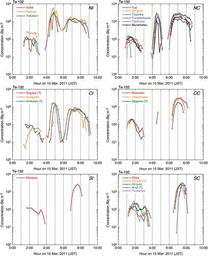
Figure 5. Same as Figure 3 but for I-131.

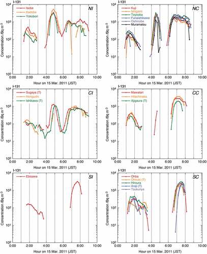
As shown in Figures 3–5, three passages of the radioactive plumes of P2A, P2B and P3C can be again identified. The concentrations newly estimated by the hybrid method have a similar tendency with respect to their concentration levels and timings of their rising and descending to those of neighboring MSs estimated by Terasaka et al. [13]. Whereas, discrepancies of about two folds in levels and several ten min in arrival/leaving times could be seen among the newly estimated variations. In the case of Plume P2B, the MSs located in SC and SI did not detect its passage for any of the five nuclides. Many of the highest concentrations of the five nuclides in each Plume are estimated at the MSs in NC and NI.

Plume P2A is first identified just before 1:00 on 15 March 2011 (JST) at the MSs in NC, and within 30 min the other MSs start to identify its arrival. It leaves the MSs by 3:00 except for those in SC and SI where it leaves by 4:00. The highest concentrations of Plume P2A are as follows: 6.80 kBq m⁻³ of Xe-133 at Kadobe in NI, 290 Bq m⁻³ of Te-132 at Araji in SC, 510 Bq m⁻³ of I-131 at Isobe in NI, 450 Bq m⁻³ of I-132 at Isobe in NI and 150 of I-133 at Hiroura in SC. As shown in Table 3, Xe-133 concentrations comparable to the highest spread somewhat evenly along NC, CC, and SC. It is again realized as Teraesaka et al. [13] that the concentrations of the radionuclides of Plume P2A are approximately one order of magnitude lower than those in Plumes P2B and P2C.

Table 3. The highest concentrations of the nuclides in each plume. Bold figures are maxima among the monitoring stations. The mark (T) following monitoring stations name means the estimation by Terasaka et al. [13].

		Xe-133/Bq m^−3			Te-132/Bq m^−3			I-131/Bq m^−3			I-133/Bq m^−3			I-132/Bq m^−3
No.	MS	P2A	P2B	P2C	P2A	P2B	P2C	P2A	P2B	P2C	P2A	P2B	P2C	P2A	P2B	P2C
	Northern Coastal (NC) sector
1	Kuji	2300	61,600	75,600	110	2930	2670	190	2820	1960	40	240	370	150	4040	3680
2	Ishigami	1600	66,700	48,700	100	1770	1580	180	2210	1550	30	240	340	130	2750	2810
3	Toyooka	4200	129,200	106,100	150	2870	3030	290	3360	2660	70	920	1040	160	2940	3190
4	Funaishikawa	2100	91,500	64,500	70	1770	1400	170	2300	1710	60	850	810	60	1100	1000
5	Oshinobe	5700	134,000	122,000	130	2170	2700	320	2760	2640	70	640	820	220	2720	3520
6	Muramatsu	3400	44,700	72,700	140	1100	1850	220	1310	1980	50	160	430	190	1760	3990
	Northern Inland (NI) sector
7	Isobe	5900	83,500	48,900	130	3440	1370	510	3590	1460	70	320	190	450	5620	2060
8	Kadobe	6700	68,200	48,800	260	6000	1840	350	5400	940	110	1620	450	180	4650	950
9	Yokobori	3200	127,700	48,300	110	2950	1520	260	3120	1110	100	1450	780	90	1700	690
	Central Coastal (CC) sector
10	Mawatari	6300	21,800	111,000	210	500	3190	400	540	2920	100	140	1120	210	420	3110
11	Hitachinaka	300	-	6100	200	-	2840	450	-	3720	120	-	980	300	-	4620
12	Ajigaura(T)	5600	-	85,800	190	-	1840	280	-	2000	60	-	390	230	-	2710
	Central Inland (CI) sector
13	Sugaya (T)	2600	81,400	48,800	100	1720	920	140	1310	850	30	290	190	110	1390	960
14	Horiguchi	2500	17,600	46,300	60	140	750	170	380	1060	40	60	400	90	350	1370
15	Ishikawa (T)	2000	57,900	42,000	100	1400	800	120	1150	820	30	270	180	90	1110	870
	Southern Coastal (SC) sector
16	Ohba	5600	-	80,200	230	-	2710	340	-	2600	70	-	510	310	-	4260
17	Ohnuki (T)	6500	-	102,100	160	-	1950	250	-	1860	60	-	540	190	-	2460
18	Hiroura	6300	-	107,300	150	-	3280	450	-	3180	150	-	1580	220	-	3570
19	Araji (T)	6100	-	105,500	290	-	2320	380	-	2300	80	-	670	270	-	2900
20	Tsukuriya	4100	-	74,700	230	-	2580	340	-	2990	80	-	890	270	-	4470
	Southern Inland (SI) sector
21	Ebisawa	3000	-	61,500	120	-	2720	170	-	3240	50	-	890	70	-	3700

Count overflows occurred at Isobe and Kadobe for Plume P2B.

Plume P2B is identified at about 4:00 in NC and NI, and 30 min later it is identified at the westernmost Ishikawa in CI. It stays for a short period of about 1 h around the MSs in NC, NI and CI. It is found that Plume P2B does not reach the MSs in CC, SC and SI, except for Mawatari, which is the most inland (the nearest to CI) in CC. As in Table 3, the highest concentrations of Plume P2B are 6.00 kBq m⁻³ of Te-132 at Kadobe in NI, 5.40 kBq m⁻³ of I-131 at Kadobe in NI, 5.62 kBq m⁻³ of I-132 at Isobe in NI and 1.62 kBq m⁻³ of I-133 at Kadobe in NI. Thus, the highest concentrations of the four radionuclies are all estimated in NI. Terasaka et al. [13] found the highest I-131 concentration of Plume P2B of 1.3 kBq m⁻³ at Sugaya MS in CI. The finding of the four folds higher I-131 concentrations in NI is one of the remarkable results of this work, with respect to their levels and locations. The axis of Plume P2B was found by this work to be located more to the northwest than the indication by Terasaka et al. [13]. The highest of the estimated Xe-133 concentrations in Plume P2B was 134 kBq m⁻³ at Oshinobe in NC and not at Kadobe or Isobe in NI where the highest concentrations of the other four radionuclides are estimated, as shown in Table 3. This would be caused by that estimation of the Xe-133 concentration is not carried out for 4:40 to 5:20 at Kadobe and for 4:40 to 5:00 at Isobe due to overflows of the10 min count records in the bin-1s of these MSs.

Plume P2C also first arrives at the MSs in NC sector about 6:00, just following P2B leaving. It stays for nearly 3 h by 9:00 in NC, NI and CI sectors, in contrast with CC, SC, and SI where Plume P2C stays for shorter periods of 1 h or less than 2 h. Leavings of Plume P2C in the latter sectors are about 8:00 and earlier than in the former three sectors. The highest concentrations of Plume P2C are 122 kBq m⁻³ of Xe-133 at Oshinobe in NC, 3.27 kBq m⁻³ of Te-132 at Hiroura in SC, 3.72 kBq m⁻³ of I-131 at Hitachinaka in CC, 4.62 kBq m⁻³ of I-132 at Hitachinaka in CC and 1.58 kBq m⁻³ of I-133 at Hiroura in SC. High Xe-133 concentrations comparable to the highest are also estimated at Mawatari in CC and Ohnuki, Hiroura and Araji in SC. The MSs in the coastal sectors mark higher concentrations, including the other four radionuclides, as Terasaka et al. [13] indicated.

3.2.2. Spatial distributions

The temporal evolutions in the spatial distribution of Xe-133, Te-132, and I-131 concentrations in the three plumes are illustrated in Figures 6–8. Those of I-133 and I-132 are in Figures S3–S5 of SOM [24].

Figure 6. The spatial distribution of atmospheric concentrations of Xe-133, Te-132 and I-131 in Plume P2A.

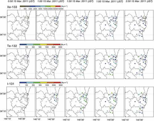
Figure 7. Same as Figure 6 but in Plume P2B.

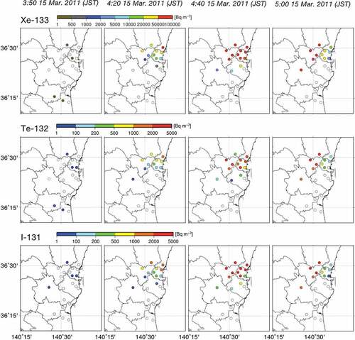
Figure 8. Same as Figure 6 but in Plume P2C.

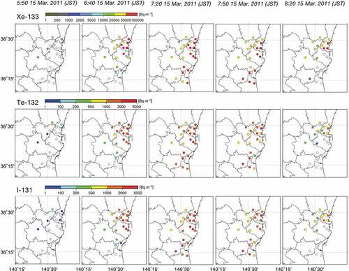
The arrival of Plume P2A is first identified at the northeasternmost Kuji MS on 0:50. As shown in Figure 6, the plume first travels southward along the coast by 1:30, and then spread to the inland area. At this time the distribution of the plume is rather uniform without any obvious axis. At 2:20 the plume begins to leave the area, whereas it seems that higher concentrations illustrated by about 100 Bq m⁻³ of I-131 still remain longer at the northernmost Isobe and the northwesternmost Kadobe. The Isobe MS has been at a lower altitude of 8 m and located just in the west of the southern end of Abukuma Highlands with more than 150 m height. There a lowland along Kuji River that flows east to the Pacific Ocean has met a valley along tributaries from Abkuma Highlands on the north side. At 2:00 the wind direction was the north-northeast (NNE) at Hitachi AMeDAS observatory (36°34.8ʹN, 140°38.7ʹE) and east-northeast (ENE) at Mito weather station (36°22.8ʹN, 140°28.0ʹE), pointed as H and M in Figure 1, respectively [25]. Based on the configuration of the Isobe MS that has been on the lowland surrounded by higher lands to the northeast, it is suggested that Plume P2A moving southward along the east coast along the foot of the Abukuma Highland went around to the lowland of Isobe and then became stagnant there. The concentration distributions seem to have been affected by the local terrain.

Plume P2B is first identified at Kadobe MS at 3:50 and then at the MSs in NI and the westernmost Ishikawa, as shown in Figure 7. The plume is distributed only in the northern part of the area of interest along a northeast-southwest axis connecting these MSs. The southern end of the distribution is from Muramatsu to Mawatari and Horiguchi. Higher concentrations of I-131 and the other nuclides are obtained at Isobe and Kadobe than those at Sugaya and Ishikawa at which concentration was previously estimated by Terasaka et al. [13]. These findings suggest that the axis of Plume P2B occurred in more inland area to the northwest. Kadobe is the northwesternmost MS where the atmospheric concentrations are estimated in this study, whereas there are some MSs where only air absorbed dose rate records are available around Kadobe [26]. The 10-min dose rates at 5:00 at Kume located at 6 km north from Kadobe (shown in Figure 1 and Table 1 as K) and Nemoto at 6 km northwest (as N) were 2612 and 3939 nGy h⁻¹, respectively, and these were less than 4883 nGy h⁻¹ at Kadobe. During the passage of Plume P2B, the dose rates at these two MSs were continuously below those at Kadobe. This result supports that the axis of Plume P2B traveled within 6 km from Kadobe.

Plume P2C is first identified at the northeasternmost Kuji at 5:50 and then moves along a north-to-south axis along the coastal area, as shown in Figure 8. After 7:50, I-131 concentrations more than 1000 Bq m⁻³ exist at the MSs in NC, whereas no significant concentrations are estimated at most of the MSs in CC and SC. Terasaka et al. [13] suggested a possibility that onshore wind of fresh maritime air without the radionuclides caused steep concentration gradients on the eastern side of the plume. At 8:00, wind direction and speed at Hitachi and Mito were NNE 3.4 m s⁻¹ and NE 6.4 m s⁻¹, respectively [24]. The temporal evolution of the spatial concentration distributions shown in Figure 8, however, reveals that the air parcel with the high I-131 concentration existing in the NC sector at 7:50 is not identified later in the southwest downwind area of the NC sector. That is, the high concentration air parcel seems to ‘disappear.’ This suggests another possibility that the onshore wind did not shift Plume P2C westward but slip under Plume P2C to keep it away vertically from the MSs on the ground.

For Plumes P2A and P2C, Xe-133 concentrations at Hitachinaka in CC are estimated to be about one order of magnitude lower than those at the other MSs in CC, while the concentrations of the other nuclides are comparable. The reason for this is not unclear at present. Inappropriate energy calibration for the lowest energy channels of the pulse height distributions of the Hitachinaka MS would be a possibility.

3.3. Radionuclide composition of the plumes

3.3.1. Concentration ratios

Table 4 shows the ratios of atmospheric radioactivity concentrations of X-133, Te-132, I-132, and I-133 to that of I-131 at the 21 MSs for each radioactive plume with their geometric means (GMs). The ratios are calculated based on time-averaged radioactivity concentrations for the periods during which concentrations of both the radionuclides meet the significance criteria mentioned in Section 2.4. The tendency shown in the ratios of time-averaged concentrations among the nuclides and the plumes are almost the same as Terasaka et al. [13].

Table 4. The activity ratios calculated from time-averaged concentrations for each plume.

		Xe-133/I-131			Te-132/I-131			I-133/I-131			I-132/I-131
No.	MS	P2A	P2B	P2C	P2A	P2B	P2C	P2A	P2B	P2C	P2A	P2B	P2C
	Northern Coastal (NC) sector
1	Kuji	10.9	28.0	37.4	0.737	1.10	1.39	0.158	0.090	0.170	0.816	1.47	1.84
2	Ishigami	10.5	32.0	36.3	0.645	0.831	1.19	0.172	0.110	0.183	0.724	1.26	2.14
3	Toyooka	15.7	43.9	39.5	0.569	0.904	1.06	0.286	0.260	0.370	0.550	0.891	1.21
4	Funaishikawa	11.6	42.2	36.0	0.394	0.815	0.772	0.329	0.367	0.439	0.323	0.469	0.567
5	Oshinobe	19.2	50.4	50.4	0.465	0.813	1.08	0.233	0.228	0.321	0.653	4.28	1.45
6	Muramatsu	15.2	39.8	35.9	0.698	0.828	0.903	0.172	0.125	0.128	0.816	1.45	1.96
	Northern Inland (NI) sector
7	Isobe	13.2	44.6	34.3	0.281	0.856	0.979	0.179	0.095	0.130	0.870	1.55	1.62
8	Kadobe	19.0	41.6	63.1	1.08	1.01	2.65	0.446	0.295	0.680	0.486	0.853	1.04
9	Yokobori	13.7	40.9	49.2	0.605	0.923	1.67	0.422	0.449	0.836	0.329	0.539	0.556
	Central Coastal (CC) sector
10	Mawatari	16.0	39.9	38.8	0.580	0.874	1.05	0.279	0.240	0.358	0.529	0.766	1.09
11	Hitachinaka	0.898	-	1.15	0.488	-	0.729	0.276	-	0.244	0.627	-	1.27
12	Ajigaura(T)	20.7	-	50.5	0.627	-	0.901	0.212	-	0.196	0.821	-	1.36
	Central Inland (CI) sector
13	Sugaya (T)	13.6	60.8	57.9	0.580	1.20	0.908	0.220	0.211	0.204	0.778	1.05	1.07
14	Horiguchi	15.1	45.2	43.9	0.411	0.420	0.594	0.246	0.195	0.366	0.582	0.923	1.22
15	Ishikawa (T)	15.2	50.8	50.6	0.703	1.11	0.845	0.226	0.225	0.199	0.708	0.966	0.988
	Southern Coastal (SC) sector
16	Ohba	15.2	-	35.3	0.749	-	1.09	0.241	-	0.136	0.828	-	1.63
17	Ohnuki (T)	24.3	-	60.7	0.487	-	1.03	0.221	-	0.257	0.653	-	1.26
18	Hiroura	12.2	-	37.9	0.439	-	1.06	0.346	-	0.481	0.483	-	1.14
19	Araji (T)	16.5	-	49.2	0.595	-	1.09	0.216	-	0.264	0.636	-	1.23
20	Tsukuriya	12.9	-	28.4	0.870	-	1.15	0.284	-	0.285	0.839	-	1.61
	Southern Inland (SI) sector
21	Ebisawa	19.4	-	21.5	0.942	-	0.852	0.301	-	0.277	0.414	-	1.15
Geometric Mean		13.2	42.3	35.0	0.589	0.876	1.04	0.250	0.199	0.272	0.617	1.07	1.24
Estimated (Terasaka et al. [13])		18.1	57.1	53.7	0.61	1.1	0.95	0.22	0.22	0.23	0.59	0.96	1.2
Measured (Ohkura et al. [1])		-	-	-	0.403	0.818	0.702	0.171	0.149	0.140	0.484	0.841	0.899

The GM of Xe-133/I-131 of Plume P2A for all the MSs are 13.2, and it is substantially less than those of 42.3 for P2B and 35.0 for P2C, although Terasaka et al. [13] calculated slightly larger ratios of 18.1 for Plume P2A, 57.1 for P2B and 53.7 for P2C from the pulse height distribution records of the limited 6 MSs. This difference between ratios by this work and Terasaka et al. [13] might suggest nonuniform spatial distributions of the radionuclides in each plume. The spatial distributions of the ratios of the radioactive nuclide concentrations are discussed in 3.3.2.

For Te-132/I-131, the GM are 0.589, 0.876 and 1.04 for Plume P2A, P2B and P2C, respectively. Plume P2A has a slightly smaller Te-132/I-131 than the others. While, for I-133/I-131, the GMs of the three plumes show almost the same values of about 0.2, but, in detail, the GM of Plume P2B is the smallest. The GMs of I-132/I-131 are 0.617, 1.07 and 1.24 for Plume P2A, P2B and P2C, respectively, and these are similar to those of Te-132/I-131, rather than those of I-133/I-131.

The GMs of Xe-133/I-131 of Plume P2B and P2C are triple or larger than that of Plume P2A, whereas for each GM of Te-132/I-131, I-133/I-131 and I-132/I-131 of Plume P2B and P2C is similar to or at most twice of the respective GM of Plume P2A. This fact highlights the unique composition of Plume P2A with less abundant Xe-133. Since both I-131 and I-133 in the plumes are fission products, they have common sources (i.e. reactor cores), and since they are isotopes of iodine, they are subject to common removal processes during their discharge from the power plant and travel in the atmosphere. Therefore, the discrepancy among the above I-133/I-131 of the plumes implies the difference in some characteristics of damaged nuclear fuels that contributed to these plumes.

Since I-132 with a half-life of 2.23 h is a decay product of Te-132 with a half-life of 3.2 d, I-132 were continuously produced in the plumes including Te-132. Since Te-132 and I-132 are not isotopes, they have different physicochemical efficiencies of removal out of the atmosphere, even if they exist in the same plume. Thus, the behavior of I-132 in the plumes must have been more complicated comparing to I-131 and I-133. More sophisticated analysis is necessary to understand the implication of the results of the I-132/I-131 ratios.

3.3.2. Temporal variations and spatial distributions

Temporal variations in the 10-min activity ratios of Xe-133/I-131 and Te-132/I-131 are depicted in Figures 9 and 10. Those of I-132/I-131 and I-133/I-131 are in Figures S6 and S7 in SOM [24]. Here, the 10-min concentration ratios were calculated by adopting the estimated concentration values that meet another criterion of the significance of >4σ instead of >3σ, since concentration ratio calculated from too low concentration values with relatively larger statistical uncertainties suffered from large fluctuations.

Figure 9. Temporal variations in the 10-min activity ratio of Xe-133/I-131. The mark (T) following each monitoring station name in the legends means calculations from the results of Terasaka et al. [13].

Figure 10. Same as Figure 9 but of Te-132/I-131.

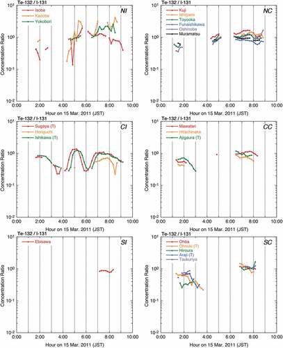
For Xe-133/I-131 and Te-132/I-131 shown in Figures 9 and 10, among most of MSs the calculated 10-min ratios show similar temporal variations and agreed within a factor of 2 to 3. While the 10-min ratios relatively less fluctuate, they seem to have week temporal trends during the passage of each plume: increases in Xe-133/I-131 at the ends of Plumes P2B and P2C passages shown in Figure 9. Whereas, Te-132/I-131 seems to increase during Plume P2B but slightly decrease during Plume P2C, as shown in Figure 10.

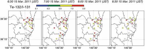
Characteristic temporal evolutions of spatial distributions of Xe-133/I-131 and Te-132/I-131 are illustrated in Figure 11 for Plume P2A and in Figure 12 for Plume P2B. For Plume P2A shown in Figure 11, higher Xe-133/I-131 of more than 20 continuously appear along the coast after 1:40, implying nuclide composition gradient in the west-to-east direction. While, Te-132/I-131 lower than 0.5 first appeared in the northern coastal area at 1:20 and then moves to the southern coastal area after 2:30. Plume P2A included a relatively Xe-133-rich and Te-132-depleted portion along the coast. Figure 12 clearly shows that first, the head of Plume P2B with lower Xe-133/I-131 arrives at the MSs in NI and NC, and after 4:50 a portion with Xe-133/I-131 higher than 50 follows the head of the plume to move to southwest. Similarly, after 4:50, a higher Te-132/I-131 portion of the plume moves from northeast to southwest. As shown in Figure 13, the fraction of the MSs with Te-132/I-131 higher than 1.0 in the all the MS in NC seems to decrease after 8:00, suggesting the tail of Plume P2C has Te-132/I-131 slightly lower than that of the head. The details of non-uniformity of the radionuclide compositions in each plume are suggested by this work.

Figure 11. The spatial distribution of Xe-133/I-131 and Te-132/I-131 in Plume P2A.

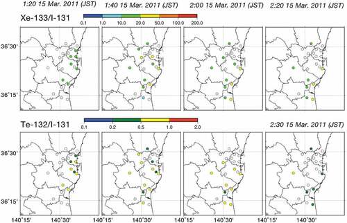
Figure 12. Same as Figure 11 but in P2B.

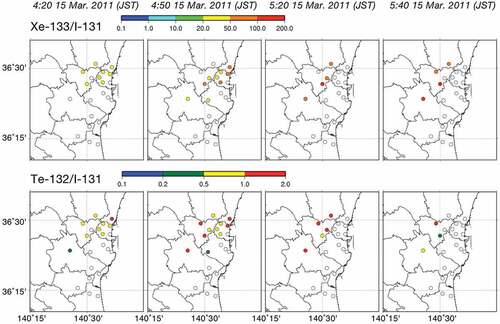
Figure 13. The spatial distribution of Te-132/I-131 in Plume P2C.

4. Conclusion

The hybrid method for estimation of atmospheric radionuclide concentrations from NaI(Tl) pulse height distributions was developed and applied to the MSs where NaI(Tl) pulse height records were available for the period on 15 March 2011 in Ibaraki Prefecture but were left not analyzed in the estimation by Terasaka et al. [13] for the reason of surrounding complex terrains and structures. The concentrations at Muramatsu estimated by the hybrid method were consistent with previous estimations by Terasaka et al. [13] and measured concentrations [1] within a factor of 2.

Temporal variations in atmospheric concentrations of I-131, I-132, I-133, Te-132 and Xe-133 in the three radioactive plumes P2A, P2B and P2C that passed over Ibaraki Prefecture in the morning of 15 March 2011 were successfully estimated for the 21 MSs, and this enabled to analyze details of spatial distributions of the plumes in the broader area than Terasaka et al. [13]. For each radionuclide the atmospheric concentrations of Plumes P2B and P2C were one order of magnitude higher than those of P2A. Higher I-131 concentration of 5.40 kBq m⁻³ during Plume P2B passage was estimated in the northwestern inland area, in comparison to the maximum of 1.3 kBq m⁻³ estimated by Terasaka et al. [13]. In the same way, higher concentrations of the other radionuclides were found in the northwestern inland area for Plume P2B. The spatial distribution analysis revealed that Plume P2A was found to have no obvious axis. The axis of Plume P2B was located more to the northwest than previously presumed, and the axis of P2C was along the coastal area from north to south. These locations of the axes of the plumes were determined with the spatial resolutions of the MS network of 10 km or less. The analysis of the temporal evolution in the spatial distributions revealed the plausible behaviors of the plumes caused by the local terrains and meteorology, such as the stagnant remaining of Plume P2A around Isobe and the migration of the radionuclide-free onshore wind under Plume P2C.

Substantially lower Xe-133/I-131 of 13.3 for Plume P2A was recognized as compared with those of 42.3 for P2B and 35.0 for P2C. Te-132/I-131 and I-132/I-131 of Plume P2A were also slightly lower than those of the other plumes. Slightly lower I-133/I-131 for Plume P2B than the others would imply a change in the relative contributions of the reactors to each plume. The non-uniformity of the radionuclide composition in each plume was recognized. Plume P2A included the relatively Xe-133-rich and Te-132-depleted portion along the coast. Plume P2B had the head portion with lower Xe-133/I-131 and Te-132/I-131 followed by the tail one with higher Xe-133/I-131 and Te-132/I-131. Plume P2C had the tail with slightly lower Te-132/I-131 than that of the head.

Acknowledgments

The authors would like to thank university students Tomoyuki Mori and Hikaru Nishiyama for their cooperation in drawing spatial distribution charts for the analysis.

Disclosure statement

No potential conflict of interest was reported by the authors.

Supplemental material

Supplemental data for this article can be accessed here.

Additional information

Funding

This work was supported by the JSPS KAKENHI [grant No. 24110002] and the ERCA Environment Research and Technology Development Fund [project No. 1-1802]].

References

- Ohkura T, Oishi T, Taki M, et al. Emergency monitoring of environmental radiation and atmospheric radionuclides at Nuclear Science Research Institute, JAEA following the accident of Fukushima Daiichi Nuclear Power Plant. Tokai-mura (Japan): Japan Atomic Energy Agency; 2012. ( JAEA-Data/Code 2012-010).
- Furuta S, Sumiya S, Watanabe H, et al. Results of the environmental radiation monitoring following the accident at the Fukushima Daiichi Nuclear Power Plant –Interim report (Ambient radiation dose rate, radioactivity concentration in the air and radioactivity concentration in the fallout)–. Tokai-mura (Japan): Japan Atomic Energy Agency; 2011. (JAEA-Review 2011-035) [in Japanese].
- Stohl A, Seibert P, Wotawa G, et al. Xenon-133 and caesium-137 releases into the atmosphere from the Fukushima Dai-ichi Nuclear Power Plant: determination of the source term, atmospheric dispersion, and deposition. Atmos Chem Phys. 2012;12:2313–2343.
- Amano H, Akiyama M, Bi CL, et al. Radiation measurements in the Chiba metropolitan area and radiological aspects of fallout from the Fukushima Dai-ichi nuclear power plants accident. J Environ Radioact. 2012;111:42–52.
- Kim E, Kurihara O, Kunishima N, et al. Early intake of radiocesium by residents living near the TEPCO Fukushima Dai-Ichi nuclear power plant after the accident. Part 1: internal doses based on whole- body measurements by NIRS. Health Phys. 2016;111:451–464.
- Kunishima N, Kurihara O, Kim E, et al. Early intake of radiocesium by residents living near the TEPCO Fukushima Dai-Ichi Nuclear Power Plant after the accident. Part 2: relationship between internal dose and evacuation behavior in individuals. Health Phys. 2017;112:512–525.
- Kim E, Tani K, Kunishima N, et al. Estimation of early internal doses to Fukushima residents after the nuclear disaster based on the atmospheric dispersion simulation. Radiat Prot Dosimetry. 2016;171:398–404.
- Kurihara O, Kim E, Kunishima N, et al. Development of a tool for calculating early internal doses in the Fukushima Daiichi nuclear power plant accident based on atmospheric dispersion simulation. ICRS-13 & RPSD-2016, EPJ Web of Conferences; Paris, France; 2017;153:08008.
- Sato Y, Takigawa M, Sekiyama TT, et al. Model intercomparison of atmospheric 137Cs from the Fukushima Daiichi Nuclear Power Plant Accident: simulations based on identical input data. J Geophys Res Atmos. 2018;123:11748–11765.
- Tsuruta H, Oura Y, Ebihara M, et al. First retrieval of hourly atmospheric radionuclides just after the Fukushima accident by analyzing filter-tapes of operational air pollution monitoring stations. Sci Rep. 2014;4:6717.
- Oura Y, Ebihara M, Tsuruta H, et al. Determination of atmospheric radiocesium on filter tapes used at automated SPM monitoring stations for estimation of transport pathways of radionuclides from Fukushima Dai-Ichi Nuclear Power Plant. J Radioanal Nucl Chem. 2015;303:1555–1559.
- Oura Y, Ebihara M, Tsuruta H, et al. A database of hourly atmospheric concentrations of radiocesium (134Cs and 137Cs) in suspended particulate matter collected in March 2011 at 99 air pollution monitoring Stations in Eastern Japan. J Nucl Radiochem Sci. 2015;15:1–12.
- Terasaka Y, Yamazawa H, Hirouchi J, et al. Air concentration estimation of radionuclides discharged from Fukushima Daiichi Nuclear Power Station using NaI(Tl) detector pulse height distribution measured in Ibaraki Prefecture. J Nucl Sci Technol. 2016;53:1919–1932.
- Hirouchi J, Yamazawa H, Hirao S, et al. Estimation of surface anthropogenic radioactivity concentrations from NaI(Tl) pulse-height distribution observed at monitoring station. Radiat Prot Dosimetry. 2015;164:304–315.
- Hirayama H, Kawasaki M, Matsumura H, et al. Estimation of I-131 concentration using time history of pulse height distribution at monitoring post and detector response for radionuclide in plume. Trans At Energy Soc Jpn. 2014;13:119–126. [in Japanese].
- Hirayama H, Matsumura H, Namito Y, et al. Estimation of time history of I-131 concentration in air using NaI(Tl) detector pulse height distribution at monitoring posts in Fukushima Prefecture. Trans At Energy Soc Jpn. 2015;14:1–11. [in Japanese].
- Tsuruta H, Oura Y, Ebihara M, et al. Spatio-temporal distribution of atmospheric radiocesium in Eastern Japan just after TEPCO Fukushima Daiichi Nuclear Power Plant Accident – analysis of used filter-tapes of SPM monitors in air quality monitoring stations –. Earozoru Kenkyu. 2017;32:224–254. [in Japanese].
- Tsuruta H, Oura Y, Ebihara M, et al. Time-series analysis of atmospheric radiocesium at two SPM monitoring sites near the Fukushima Daiichi Nuclear Power Plant just after the Fukushima accident on March 11, 2011. Geochem J. 2018;52:103–121.
- Ibaraki Prefectural Government [Internet]. Japan: Ibaraki Prefecture; 2013 Mar 21 [cited 2019 Jun 17]. Available from: http://www.pref.ibaraki.jp/seikatsukankyo/gentai/anzen/nuclear/radiachion/mca.html [in Japanese].
- Hirayama H, Matsumura H, Namito Y, et al. Estimation of Xe-135, I-131, I-132, I-133 and Te-132 concentrations in plumes at monitoring posts in Fukushima Prefecture using pulse height distribution obtained from NaI(Tl) detector. Trans At Energy Soc Jpn. 2017;16:1–14. [in Japanese].
- Hirayama H, Namito Y, Bielajew AF, et al. The EGS5 code system. Tsukuba (Japan): High Energy Accelerator Research Organization (KEK), Stanford Linear Accelerator Center (SLAC); 2005. (KEK Report 2005-8, SLAC-R-730).
- Namito Y, Nakamura H, Toyoda A, et al. Transformation of a system consisting of plane isotropic source and unit sphere detector into a system consisting of point isotropic source and plane detector in Monte Carlo radiation transport calculation. J Nucl Sci Technol. 2012;49:167–172.
- Casanovas R, Morant JJ, Salvadó M. Energy and resolution calibration of NaI(Tl) and LaBr3(Ce) scintillators and validation of an EGS5 Monte Carlo user code for efficiency calculations. Nucl Instr Meth Phys Res A. 2012;675:78–83.