
ABSTRACT
After direct discharges of highly contaminated water of the Fukushima Daiichi Nuclear Power Plant (1 F) from April to May 2011, Kanda suggested that relatively small amounts of run-off of radionuclides from the 1 F port into the Fukushima coastal region subsequently continued by his estimation method. However, the estimation period was limited to up to September 2012. Therefore, this paper estimatesthe discharge inventory up to June 2018. In the missing period, the Japanese government and Tokyo Electric Power Company Holdings have continued efforts to stop the discharge, and consequently, the radionuclide concentration in seawater inside the 1 F port has gradually diminished. We show the monthly discharge inventory of 137Cs up to June 2018 by two methods, i.e., Kanda method partially improved by the authors and a more sophisticated method using Voronoi tessellation reflecting the increase in the number of monitoring points inside the 1 F port. The results show that the former always yields overestimated results compared with the latter, but the ratio of the former to the latter is less than one order of magnitude. Using these results, we evaluate the impact of the discharge inventory from the 1 F port into the coastal area and radiation dose upon fish ingestion.
1. Introduction
During the accidents [Citation1–Citation3] in the Fukushima Daiichi Nuclear Power Plant (1 F) operated by Tokyo Electric Power Company Holdings (TEPCO), large amounts of radioactive materials were released into the environment, and some were deposited on the ground and sea surfaces through atmospheric diffusion [Citation1–Citation3]. Since the element caesium (Cs) has the unique property of being strongly fixed to soil clay minerals [Citation4], radioactive Cs settled on the ground has remained in the soil’s top surface layer, and consequently, this has resulted in high air-dose rates in the area around 1 F over a long period of time [Citation4]. On the other hand, radionuclides deposited onto the sea’s surface temporarily raised the radionuclide concentration in surface seawater, and subsequently, surface-layer fish showed high concentrations of radioactive Cs. However, due to characteristic seawater flows such as the coastal and ocean currents off the coast of Fukushima, the radionuclides were widely dispersed, and the seawater concentration decreased rapidly [Citation5–Citation8].
In addition to the environmental release from 1 F via atmospheric diffusion, a significant amount of contaminated water accumulated inside the reactor building was discharged directly into the ocean [Citation9]. The discharge from the Unit 2 intake pit was the largest in the visible range, followed by that from Unit 3 along with the planned release of low-concentration contaminated water. Since all discharges (except the planned release) were via the 1 F port, it is considered that once radioactive materials stayed inside the port, they spread outside the port, eventually toward the coast and Pacific Ocean [Citation10]. This paper focuses on 137Cs, which is one of the most crucial radionuclides released via the 1 F port and estimates the discharge inventory from the port over the seven years from April 2011 to June 2018 with discussing associated temporal variations. In addition, the impacts on the Fukushima coastal marine environment from the estimated continuous discharge are evaluated, i.e., the effects on coastal seawater concentrations, and related human exposure via the consumption of fish contaminated by the estimated discharge amounts are assessed.
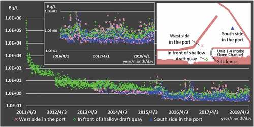
After the contaminated water leak in the early stages of the 1 F accident, the Japanese government and TEPCO prepared a system to continuously purify the contaminated water accumulated inside the reactor building [Citation11], and simultaneously launched and implemented various countermeasures to stop the run-off of the contaminated water into the ocean [Citation11]. Because of these efforts, the monitoring results revealed that the concentration of 137Cs inside the port decreased by a factor of 100,000 in August 2018 compared with the 2011 initial period at the measurement point termed ‘In front of shallow draft quay’, which is located in the central part of the port revetment as shown in [Citation11,Citation12]. The decrease rate was highest at the beginning of the accident, and it subsequently slowed down, but the decreasing tendency has continued. However, the radionuclide concentration inside the 1 F port remains higher than outside the port, and moreover, there is a concentration gradient inside the port as shown in , which displays seawater concentrations at two other points termed ‘West side in the port’ and ‘South side in the port’ in addition to ‘In front of shallow draft quay’. This suggests that it remains essential to continue the internal and external monitoring of the 1 F port and to observe the spatial and temporal variations in the concentrations inside the port as long as such circumstances persist.
Figure 1. Seven-year temporal variation of 137Cs seawater concentrations (Bq/L) at the monitoring point termed ‘In front of shallow draft quay’, ‘West side in the port’, and ‘South side in the port’ displayed in the right-hand-side insert figure. The left-hand-side insert figure is an enlarged view of a part of the main figure.
This paper focuses on 137Cs which has a long half-life of 30 years and relatively long-term environmental impacts, and estimates the discharge inventory of 137Cs from the 1 F port based on the monitoring data from inside the port [Citation13]. To date, such an attempt has been limited only to a paper by Kanda [Citation13]. Moreover, the report period of the discharge of 137Cs was limited to the early stages of the accident up to September 2012. There has been no subsequent report, and all other papers have attempted discharge estimations by using monitoring data obtained from outside the port [Citation6–Citation8,Citation14]. Therefore, this study estimates the missing discharge inventory over the seven years from the early stages of the accident to the most recent one in June 2018 using both the same approach as well as more improved ones and assesses the environmental impacts.
The data used in this paper is limited to the seawater concentrations inside the 1 F port, which were measured and published by TEPCO. For the purpose of the discharge inventory estimation, this study applies the following two methods. The first is the same method used to estimate the discharge from 3 April 2011 to the end of September 2012 as suggested in Kanda’s paper (referred to Kanda method [Citation13] below). Kanda regarded the concentration of 137Cs at a measuring point, ‘In front of shallow draft quay’ as a representative of 137Cs concentration inside the port, estimated the inventory inside the port, and calculated the discharge inventory from the port using the seawater exchange rate between the inside and the outside of the port estimated separately in the same paper [Citation13]. This study follows this method but makes an additional improvement (see Section 2). This is because seawater concentration has further decreased, and its temporal fluctuation has become more intense since the period estimated by Kanda. Generally, the Kanda method [Citation13] overestimates the representative seawater concentration inside the port, because its focus point is located in the immediate vicinity of the land, which is expected to show relatively high concentrations compared with other sites further away (see ). Therefore, it should be noted that the method corresponds to one of conservative estimations. After August 2013, TEPCO started to publish monitoring results at multiple locations inside the port (see and ) [Citation15], which revealed that there were clear spatial variations in the interior concentrations. Since then, the inventory inside the port can be estimated with higher accuracy using measurement data obtained at these multiple sites. Then, this paper estimates the inventory inside the port by adopting the Voronoi tessellation method [Citation16] which uses all the concentration data of multiple monitoring points and compares its results with those generated by the Kanda method (see Section 3).
The contents of this paper are as follows. Section 2 presents the details of the Kanda method for the discharge inventory estimation, and the improvements employed in this paper are explained along with some problems inherent in the original method. Then, estimated data (the monthly discharge inventory) from October 2012 to June 2018 using the improved Kanda method is presented, which includes a period not reported since Kanda’s paper. Based on the temporal variations estimated by the improved Kanda method, characteristics of the temporal variation trends are discussed [Citation17]. Section 3 explains the new method suggested by the present authors, i.e., the inventory analysis method using Voronoi tessellation [Citation16], and also discusses the temporal variation trends in the estimated inventory. Section 4 presents the annual discharge inventories from 2011 to 2018 by adding up the estimated monthly inventories obtained in Sections 2 and 3, discussing how the concentration level rises in the Fukushima coastal area in relation to the discharge amounts, and evaluating human exposure via ingestion of marine fish.
2. Evaluation of the discharge inventory of 137Cs from the 1 F port using the Kanda method
This section concentrates on the Kanda method. Subsection 2.1 presents the method’s technical problems and suggests some improvements. In Subsection 2.2, estimated results up to June 2018 are reported using the improved version. Subsection 2.3 analyzes temporal variations of the discharge inventory over the seven-year period and discusses reasons for their occurrence.
2.1. The Kanda method and its improvement
There are two essential points in the discharge inventory estimation suggested in Kanda’s paper [Citation13]. The first is that the exchange rate of seawater between the inside and the outside of the 1 F port was determined based on the 137Cs-concentration decrease process, which was clearly observed at the beginning of the accident. The second is that the total inventory inside the port was estimated using the concentration only at ‘In front of shallow draft quay’ (see ), i.e., by regarding it as the representative site inside the 1 F port. This study follows these two points and partly improves by taking account of circumstantial changes inside the port after 2012.
The improvements to the original method are explained below. When the concentration at ‘In front of shallow draft quay’ is used as the representative one inside the 1 F port, a question arises: is the particular location valid in estimating the entire inventory inside the port? ‘In front of shallow draft quay’ is very close to the land, and therefore, its concentration is expected to be relatively higher compared with the central area and other zones inside the port except for the rectangular area referred to ‘Open channel’ (see : seawater inside ‘Open channel’ is effectively retained by the silt fence, and consequently, the ‘Open channel’ area exhibits different behaviors to the other port areas). This shows that the estimated inventory is always overestimated (see : the concentration at ‘In front of shallow draft quay’ always tends to be higher than the other two points, ‘West side in the port’ and ‘South side in the port’). Therefore, the use of monitoring data at other points inside the port is necessary to improve the accuracy of the inventory estimation inside the port. An attempt to improve the accuracy using those data is presented in the next section in more detail. As mentioned above, the Kanda method always conservatively overestimates the inventory inside the port, but it is a very simple and useful tool for assessing environmental impacts (its accuracy is discussed in Section 3). Another problem is how to treat the data in cases when the measurement concentration is less than the detection limit. Even in the early stages of the accident when Kanda estimated the inventory, the published data was occasionally below the detection limit. In such cases, the unknown value was interpolated using temporary surrounding values. However, since the observed concentration during the initial period was so sufficiently high, no major problem arose in terms of the accuracy of the inventory estimation. Conversely, since the frequency of measurement value being below the detection limit has increased and the concentration has largely fluctuated day-to-day after 2012 (see ), the estimation error has been non-negligible. shows the frequency ratio (the number of measurements when observations were below the detection limit/the total number of measurements) in every month. Up to 2012, although the frequency below the detection limit was relatively lower, the frequency increased over time. To cope with such circumstantial changes, TEPCO has occasionally lowered the detection limit, and its frequency has been reduced accordingly. However, since the concentrations always tend to decrease and the concentration itself also largely fluctuates from day-to-day, the problem remains.
Figure 2. Temporal variation of the monthly frequency in which the measurement result was beneath the detection limit whose application period is displayed along the upper arrows.
In order to solve the above problem, this study estimates the width between the detection limit value and zero, as the value is below the detection limit. The true concentration value certainly lies between the detection limit and zero. Specifically, the monthly and annual averages are calculated using both the detection limit and zero values, assuming that the true averaged value is also within the maximum and minimum range averaged by using the two values. Hereafter, the Kanda method of adopting this technique is referred to as the improved Kanda method, in which the estimated value is not uniquely determined, and the width (with the maximum and minimum values) is given instead.
2.2. The discharge inventory estimation up to June 2018 using the improved Kanda method
This subsection presents the results of the discharge inventory estimated using the improved Kanda method. First, the inventory evaluation formula of the original Kanda method is expressed. According to Kanda’s paper [Citation13], the daily discharge amount of a radionuclide from the port is given by the following formula:
The seawater volume inside the port (see : the area of the 1 F port except for ‘Open channel’) and the exchange rate applied in Kanda’s paper are also used in the present improved method. It should be noted that the seawater exchange rate (/day) is estimated by the clear decreasing trend of the high-concentration seawater observed at the beginning of the accident, i.e., the rate is supported by actual measurement data. When using this formula (1), if a value above the detection limit is measured, the observed concentration value is directly substituted into (1) as in the original method13). However, if it is below the detection limit (as described in Subsection 2.1) both the detection limit (maximum value) and zero (minimum value) are substituted into the formula (1) to obtain a set of two values with their widths. The monthly discharge inventory obtained by the above method is shown in , and the temporal variation of the estimated monthly discharge inventory is presented in . We note that all monthly estimates in have two values, i.e., the maximum and minimum values.
Table 1. Monthly estimation of the discharge inventory of 137Cs (Bq/month) using the improved Kanda method (partly improved by the authors) in the period from April 2011 to June 2018.
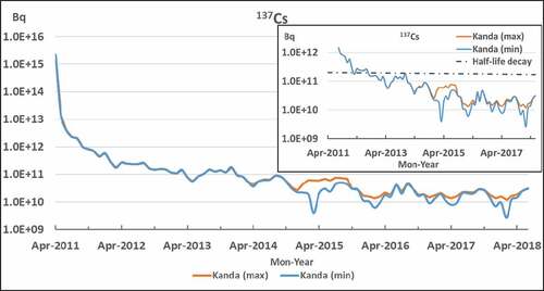
Figure 3. Main panel: Seven-year temporal variation of monthly estimation of the 137Cs discharge inventory from the 1 F port by using the improved Kanda method (partly improved by the authors) in the period from April 2011 to June 2018, and inserted one: Focused variation of the main panel.
2.3. Analysis of the discharge inventory fluctuations estimated by the improved Kanda method
Here, the temporal characteristics of the estimated discharge inventory detailed in over the period of about seven years are analyzed. First, the inventory decay was found to be very rapid immediately after the direct leak of high-concentration contaminated water early in the accident. This fast decay is considered to be caused by the outward transportation via seawater exchange between the inside and the outside of the 1 F port mainly according to alternating tidal currents. However, the decay process did not monotonously continue until the pre-accident level, of which the concentration is regarded to be the same as the background level, i.e., after decreasing to a certain inventory level, a slow decay process is found to dominate. If a constant steady discharge inventory remains in the system after the fast decay, its decay should simply be governed by its physical half-life. However, the actual decay is rather faster than the physical half-life, as seen in the inset of . This is either because the inventory source itself decreased or because the countermeasures suppressed steady discharge flux into the port. Indeed, it is noted that the concentration of the accumulated contaminated water itself decreased due to purification system operation, and some countermeasures (such as seabed covering and sea-side impermeable wall closure) have suppressed the discharge flowing into the port. However, since counter-operations that offset these suppressions have been implemented (like the relocation of the drainage channel outlet from the outside to the inside the port), it is difficult to definitively link the decreasing trends with such treatments and countermeasures. In addition, since around 2016, the seawater concentrations inside the port have strongly fluctuated, and clear seasonal variations have been recorded (see : Inset). Such seasonal variations are discussed in Section 3 in more detail.
3. Evaluation of the discharge inventory of 137Cs from the 1 F port using Voronoi tessellation
Since the Kanda method [Citation13] always overestimates the discharge inventory from the 1 F port by regarding the monitoring value of ‘In front of shallow draft quay’ as representative of inside the 1 F port, this study suggests an alternative estimation method that takes account of the monitoring values at multiple points including ‘In front of shallow draft quay’ for the purpose of improving the estimation accuracy. Since August 2013, the monitoring of seawater concentration has been extended to cover the whole 1 F port by measuring at multiple locations compared with only ‘In front of shallow draft quay’ [Citation15] in the initial period following the accident. Thus, such an expansion of the monitoring process made it possible to estimate the inventory inside the 1 F more accurately by considering the spatial distribution, including those points. For the purpose of improving the accuracy, this paper applies the Voronoi tessellation method [Citation16]. The approach considers the seawater concentrations at multiple monitoring points and estimates each inventory inside each Voronoi polygonal column by taking the product of the measured concentration, the average water depth, and the surface area in each Voronoi column. The sum of the inventories in all the Voronoi polygonal columns corresponds to the total inventory inside the port. By multiplying the calculated total inventory value inside the port by the daily seawater exchange rate of 0.44 (/day) (Kanda [Citation13] derived from the concentration decreasing process observed just after the direct-release accident), the port’s discharge inventory can be estimated. The details of the method are explained in Subsection 3.1. Subsection 3.2 shows the temporal variations of the estimated monthly discharge inventory from April 2011 to June 2018 and compares them with those obtained using the improved Kanda method. Subsection 3.3 analyzes temporal variation trends of the discharge inventory estimated by the present method. As is evident in , although the concentration at each point inside the port fluctuates, there is always a certain concentration gradient among the points inside the port, which indicates an almost steady situation. This fact confirms the validity of this study’s main estimation scheme, i.e., multiplying the seawater exchange rate by the total inventory inside the port.
3.1. Inventory estimation method using Voronoi tessellation
This section describes how the seawater concentration monitoring process inside the 1 F port has been expanded. From 3 April 2011 to the end of May 2013, the number of monitoring points inside the port was limited to only a few sites (‘In front of shallow draft quay’ and ‘Port entrance’ [Citation15]). Since August 2013, the number of monitoring points has increased to eight. Therefore, the spatial concentration distribution inside the port has become somewhat visible [Citation15]. schematically shows a history of the monitoring process inside the 1 F port.
Figure 4. Changing history of monitoring points inside the 1 F port: (a) from April 2011 to May 2013 and (b) from August 2013 to July 2018. [Base map data: Website of The Geospatial Information Authority of Japan. (http://www.gsi.go.jp/ENGLISH/index.html)].
![Figure 4. Changing history of monitoring points inside the 1 F port: (a) from April 2011 to May 2013 and (b) from August 2013 to July 2018. [Base map data: Website of The Geospatial Information Authority of Japan. (http://www.gsi.go.jp/ENGLISH/index.html)].](/cms/asset/d79018f2-6e0f-475b-af7e-262bd7ed2913/tnst_a_1740809_f0004_oc.jpg)
As reveals, during the period when Kanda [Citation15] estimated the discharge inventory, the site, ‘In front of shallow draft quay’ was found to be only a monitoring point inside the port because of initial monitoring limitations. Conversely, owing to an increase in the number of monitoring points after August 2013, the seawater concentration distribution patterns inside the port have become clear. Thus, Voronoi tessellation [Citation16] is applied in this study to estimate the inventory in each Voronoi polygonal column by regarding each monitoring site as a representative point inside each column after August 2013. Their total sum is then taken as the whole inventory inside the port. The actual Voronoi tessellation inside the port is shown in . Before June 2013, due to the monitoring site limitations described above, the data from ‘In front of shallow draft quay’ is allocated to each Voronoi polygonal column (see ). Therefore, before June 2013, the Voronoi tessellation method is equivalent to the Kanda method, but after August 2013, the estimation can be performed by adding the inventories in multiple Voronoi polygonal columns. Thus, the whole inventory accuracy inside the port has been significantly improved since August 2013.
3.2. Temporal variations of the discharge inventory by the estimation method using Voronoi tessellation
shows the monthly discharge inventory estimated using the Voronoi tessellation method, and plots its temporal variations along with those of the improved Kanda method. As shows, both the temporal variations are clearly characterized by the width between the maximum and minimum values except when high-concentration seawater was observed immediately after the accident. This indicates that the true average value lies between the maximum–minimum values as the observed 137Cs concentration often falls below the detection limit as explained in Section 2. In the Voronoi tessellation method, since multiple Voronoi polygonal columns frequently simultaneously have maximum and minimum values, the width obtained by adding their values usually becomes wider than that in the improved Kanda method.
Table 2. Monthly estimation of the discharge inventory of 137Cs (Bq/month) using the Voronoi tessellation method in the period from April 2011 to June 2018.
Figure 5. Main panel: Seven-year temporal variation of monthly estimation of the 137Cs discharge inventory from the 1 F port by using the Voronoi tessellation method with the Kanda method (minimum estimation only) in the period from April 2011 to June 2018 and inserted one: Focused variation of the main panel.
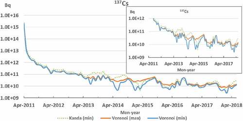
As seen in , the Voronoi tessellation method significantly exhibits smaller values than the improved Kanda method. This is because the concentration around ‘Port entrance’ is generally lower than that around ‘In front of shallow draft quay’, and the Voronoi tessellation method directly takes account of such spatial gradients and distributions. However, when comparing the inventory amounts obtained by both the improved Kanda and the Voronoi tessellation methods, a ratio of the median values from both approaches is found to be approximately within one digit, i.e., the order estimated by both methods is almost equal. This indicates that the improved Kanda method is also useful because of its methodological simplicity.
3.3. Analysis of fluctuation factors in the discharge inventory (estimated by the Voronoi tessellation)
This section analyzes the temporal variation trends of the discharge inventory. The median value between the maximum and minimum values estimated by the Voronoi tessellation method is generally lower than that of the improved Kanda method, while the widths occasionally overlap (as seen in ). This is because the maximum and minimum values in the Voronoi tessellation method tend to be overestimated more and underestimated less than in the improved Kanda method, respectively, as the seawater concentrations are below the detection limit at multiple points. However, the maximum values of the Voronoi tessellation method hardly exceed the maximum values of the improved Kanda method and vice versa. This clearly indicates that the accuracy is improved.
The temporal trends in the results obtained by the Voronoi tessellation method are qualitatively equivalent to those in the improved Kanda method. However, the temporal fluctuation estimated by the Voronoi tessellation method is more intense than that of the improved Kanda method, since the maximum–minimum width estimated by the Voronoi tessellation method is generally larger. The reason is that the Voronoi tessellation method includes more information from multiple monitoring points, some of which are located around the center zone of the port and frequently show concentrations below the detection limit. As observed in the improved Kanda method, it is found that in the Voronoi tessellation method the median values generally tend to be higher in summer and lower in winter despite the presence of the methodological fluctuation enhancements. Such seasonal variations are analogous to those observed for dissolved 137Cs in rivers [Citation18]. In the rivers that flow around 1 F, it has been pointed out that the decomposition of organic matter retaining 137Cs is promoted by high summer water temperatures, and hence, the amount of dissolved 137Cs in the water increases [Citation18]. It may be one of factors causing the seasonal variations in the 137Cs discharge inventory from the 1 F port. Since the semi-closed area inside the port is considered to be highly susceptible to seasonal temperature variations unlike in the open ocean, a similar mechanism may be responsible for the observed seasonal fluctuation. However, its supply route and the dynamics of the 137Cs carriers in such areas are not sufficiently understood. Therefore, further detailed research will be required in the future. If the seasonal variation factor of the concentration of 137Cs is elucidated, various control measures can be implemented since the 1 F port area is more controllable unlike in the case of rivers. Therefore, the factor survey is expected to greatly contribute to the suppression of the discharge of radionuclides from the 1 F port.
4. Influences of the estimated discharge inventory on the Fukushima coastal area: seawater concentration and internal exposure
Based on the results obtained in Sections 2 and 3, shows a comparison between the annual discharge inventories estimated by the two methods. From , the estimated discharge amounts in the first year after the accident are exceptionally large, and the difference between the two methods during the same period is quite small. However, from the second year, a comparison of the estimated results reveals that the median values obtained by the Voronoi tessellation method are about 50% to 85% of those from the improved Kanda method.
Table 3. Comparison of annual estimations of the 137Cs discharge inventory (Bq/year) from the 1 F port by using two methods, one of which is the improved Kanda method (partly improved by the authors) and another of which uses the Voronoi tessellation method.
Focusing on annual discharge amounts in the Voronoi tessellation method, the 2017 discharge inventory decreased by about 1/10,000 compared with that of 2011. The initial decay was very rapid, while the subsequent decay process was much slower. However, it should be noted that the decay speed is much faster than that of the half-life of 137Cs. This fact clearly indicates that suppression countermeasures or source depressions have actually contributed to the faster decay.
These countermeasure effects are assessed in more detail in this section. First, after the prevention of the significant direct discharge at the early time of the accident, a list of the potential discharge processes and sources are presented as follows,
Steady discharge into the port via groundwater leakage, including contaminated water,
Steady discharge due to the elution from deposited and subsequently adsorbed seabed-soils inside the port,
Fluctuating discharge into the port via rainfall water etc. from the catchment basin inside the 1 F site mainly through the drainage systems.
Regarding (i), owing to the sea-side impermeable wall’s closure on 26 October 2015 [Citation19], an inventory reduction inside the port was explicitly observed ( shows a clear discontinuous decrease in seawater concentrations at that time). The decrease is expected to be considerable in monthly and annual discharge, but the decrease is less significant when viewing the variation over the seven-year period. Although the influence of (ii) is also expected to be significant, no clear change has been observed despite the completion of its primary covering of the entire seabed inside the port at the end of April 2015 [Citation20]. In terms of (iii), due to the relocation of the drainage outlet from the outside the port to the inside in May 2015 [Citation21], a clear increase in the inventory inside the port is expected. However, as can be seen from , they are not clearly apparent. Therefore, the inventory variations due to (ii) and (iii) are considered to cancel each other out, because the drainage channel exit relocation was performed just after the completion of the seabed soil covering. Presently, since countermeasures(i) and (ii) are almost completed, proactive implementation of suppression measures for (iii) is hoped.
Finally, influences of the 2014 annual discharge inventory on the seawater in an entire coastal area of Fukushima (as displayed in as an example) are briefly examined. The target area is 100 km from north to south, it is centered on the 1 F port and is 20 km away from the shore (as illustrated in ). The area is approximately 2 × 10⁹ m2 (100 km × 20 km), and the total seawater capacity is estimated to be approximately 1 × 10¹¹ m3 (1 × 10¹⁴ L) by considering the deepest water depth (~100 m) in the area, which is the depth at around 20 km from shore. The background 137Cs concentration in this area was ~ 2.0 mBq/L (corresponding to the seawater concentration before the accident), but after the accident it was maintained at around 14.0 mBq/L during 2013–2015 [Citation22]. After that period, although decay occurs, it is known that the decay is very slow. Conversely, the area more than 20 km further east offshore maintains a background level even after the accident [Citation23,Citation24]. Then, if it is assumed that the discharge to the sea of the 137Cs inventory from the 1 F port in 2014 (see 3.0–4.5 × 10¹¹ Bq in ) spreads and maintains uniformity (however, since it is known that diffusive mixing actually happens further beyond the area over the year [Citation25], this assumption is a conservative assumption), only about 3.0–4.5 mBq/L is found to be added to the background level concentration 2.0 mBq/L. However, due to the above observation fact, (i.e., levels of about 14.0 mBq/L have been widely observed in the area) it is very difficult to maintain the inventory of the coastal sea area only using the discharge inventory data from the 1 F port. Therefore, more dominant inputs other than solely the 1 F port are required. This clearly suggests that it is necessary to consider the additional discharge supplied by rivers, seabed soil, and other coastal components. It was recently highlighted that the concentration of 137Cs in coastal groundwater is unexpectedly high and might provide an important contribution to the coastal inventory [Citation22]. Hence, in the future, detailed inventory assessments of coastal waters will be an important research issue.
Figure 6. Schematic figure for the coastal region around the 1 F port, in which the white line roughly indicates 20 km range distant from the land and median values of measured seawater concentrations of 137Cs are displayed for the corresponding areas. [Map data: Google, ZENRIN].
![Figure 6. Schematic figure for the coastal region around the 1 F port, in which the white line roughly indicates 20 km range distant from the land and median values of measured seawater concentrations of 137Cs are displayed for the corresponding areas. [Map data: Google, ZENRIN].](/cms/asset/1393a427-05f2-4986-8197-fe9d2a74f471/tnst_a_1740809_f0006_b.gif)
Next, the influence of 137Cs only from the 1 F port is briefly assessed in terms of human impacts. Considering that internal exposure by the consumption of marine fish in this coastal area is a major human impact, the internal dose is estimated. First, for comparison, the annual dose at the background level in this coastal area is estimated to be 1.3 × 10⁻⁴ mSv. This is because the exposure dose is 1.3 × 10⁻⁵ mSv per unit Bq in 137Cs for adults (2.0 × 10⁻⁵ mSv for children under three years of age) [Citation23,Citation26], and 10 Bq (= 2.0 mBq (B.G.)/kg × 100 × 50 kg) is annually ingested, resulting in an exposure dose of 1.3 × 10⁻⁴ mSv, as the concentration factor to fish is evenly assumed to be 100 [Citation27] and 50 kg of fish originating from this coastal area are assumed to be eaten per year. Based on this assessment, the exposure dose of the discharge of 137Cs from the 1 F port in 2014 is estimated to be 1.5 to 2.3 times the above dose, which generates an exposure dose of 1.95 to 2.93 × 10⁻⁴ mSv. Consequently, the exposure dose (originating only from the discharge of 137Cs from the 1 F port in 2014) due to the consumption of marine fish is approximately 1/1,000 lower compared with the internal dose of 0.3 mSv/year from natural radiation sources (from 40 K, U, and Th series elements). This represents an almost negligible level [Citation23,Citation26]. For marine products, the standard limit of 100 Bq/kg was set based on the internal dose for the sum of 137Cs and 134Cs. If the concentration factor and the contribution to the coastal sea concentration are also assumed to be 100 and 3.0–4.5 mBq/L, respectively, the contribution to fish from the 1 F port discharge of 137Cs inventory is found to be 0.3–0.45 Bq/kg as described above. This results in a level far below the regulation value.
However, the above evaluation assumes that the discharge of 137Cs from the 1 F port was uniformly diffused and was retained in the water inside the area 100 km north to south and 20 km offshore (as illustrated in ). Here the seawater concentration is generally not so uniform due to the non-uniformity of seawater advection/diffusion. Moreover, if hot-spots of high concentrations are localized, and if high-concentration marine fish rarely appears due to its growth around the hot-spots, such evaluations as those described above are found to be not easy issues. Therefore, it is important to prevent the migration of marine fish living inside hot-spots of relatively high-concentration (like the 1 F port) and to pay attention to the distribution of concentrations of radioactivity [Citation28] Indeed, various measures have been implemented to prevent the migration of marine fish from the 1 F port [Citation29,Citation30]. Since April 2015, no cases exceeding the standard limit of 100 Bq/kg (wet) have been observed in national and prefectural monitoring surveys [Citation31,Citation32], outside the 1 F port. According to TEPCO survey, there were partial excesses only in fish estimated to have migrated from the port [Citation33,Citation34]. However, it is difficult to conclude that those were inside the port. Nevertheless, the concentration inside the 1 F port is still higher compared to outside areas, and concentration gradient exists between the inside and the outside of the port. Therefore, it is essential to continue to monitor concentrations of both seawater and marine products and to carefully pay attention to the distribution of them and the associated temporal variations.
5. Conclusion
This paper estimated the discharge inventory of 137Cs from the 1 F port to the Fukushima coastal area and analyzed its temporal changes over the seven-year period up to June 2018. As estimation approaches, the improved Kanda method, and the Voronoi tessellation method were applied and compared. The former used only data from the site referred to ‘In front of shallow draft quay’ as the representative point inside the port, while the latter estimated the inventory using multiple monitoring points inside the port. Although the Kanda method always overestimates, the estimated amount ratio (the former/the latter) is within one digit. Hence, it was confirmed that the former is sufficiently useful owing to its methodological simplicity, while the latter is more accurate at the expense of its complexity. As the seawater concentration decreases over time and the observation frequency below the detection limit increases, both methods estimated the width between the maximum and minimum values based on the fact that there is a true value between the detection limit value and zero. The analysis of temporal variations over the seven-year period indicated that the decay process immediately after the accident was very fast owing to seawater advection/diffusion, and a very slight discharge has since continued with relatively slow decay and significant fluctuations. The difficulties involved in suppressing such slight discharge processes were found. However, although the decay of the slight discharge is very slow, it is significantly faster than that of the physical half-life. Thus, this study proposed that the conditions inside the 1 F port have recently entered into a phase, in which the discharge inventory depends on environmental factors (such as seasonal temperature variations seen in other environments, e.g., rivers, dam, lakes, etc.). In addition, from the estimated annual discharge inventory, it was found to be difficult to maintain the coastal concentration only by the discharge inventory from the 1 F port. This clearly indicates that there are other dominant inventory sources. Furthermore, if the discharge inventory from the 1 F port spreads and uniformly remains in the coastal area, its contribution to the human internal dose via the consumption of marine fish is negligible.
Note (Added Only to the Present Translated Version)
In both the original paper (in Japanese) and the present translated version, we wrote “Since April 2015, no cases exceeding the standard limit of 100 Bq/kg (wet) have been observed in national and prefectural monitoring surveys outside the 1F port”. However, after we wrote the original paper, an ocellate spot skate (Okamejei kenojei) exceeding the standard limit was caught in January 2019.
Disclosure statement
No potential conflict of interest was reported by the authors.
References
- Yamazawa H, Hirao S. Impacts of Fukushima Daiich NPP accident through atmospheric environment. J Atomic Energy Soc Jpn. 2011;53:479–483. [in Japanese].
- Chino M, Nakayama H, Nagai H, et al. Preliminary estimation of release amounts of 131I and 137Cs accidentally discharged from the Fukushima Daiichi Nuclear Power Plant into the atmosphere. J Nucl Sci Technol. 2011;48:1129–1134.
- Katata G, Chino M, Kobayashi T, et al. Detailed source term estimation of the atmospheric release for the Fukushima Daiichi Nuclear Power Station accident by coupling simulations of an atmospheric dispersion model with an improved deposition scheme and oceanic dispersion model. Atmos Chem Phys. 2015;15:1029–1070.
- Okumura M, Kerisit S, Bourg IC, et al. Radiocesium interaction with clay minerals: theory and simulation advances post–Fukushima. J Environ Radioact. 2018;189:135–145.
- Nakano M. Long-term impact on the marine environment – simulation of the marine dispersion of released radionuclides from Fukushima-Daiichi nuclear power plant and estimation of internal dose from marine products. J Atomic Energy Soc Jpn. 2011;53:559–563. [in Japanese].
- Kawamura H, Kobayashi T, Furuno A, et al. Preliminary numerical experiments on oceanic dispersion of 131I and 137Cs discharged into the ocean because of the Fukushima Daiichi Nuclear Power Plant disaster. J Nucl Sci Technol. 2011;48:1349–1356.
- Kobayashi T, Nagai H, Chino M, et al. Source term estimation of atmospheric release due to the Fukushima Dai-ichi Nuclear Power Plant accident by atmospheric and oceanic dispersion simulations. J Nucl Sci Technol. 2013;50:255–264.
- Tsumune D, Tsubono T, Aoyama M, et al. Distribution of oceanic 137Cs from the Fukushima Dai-ichi Nuclear Power Plant simulated numerically by a regional ocean model. J Environ Radioact. 2012;111:100–108.
- Nuclear Emergency Response Headquarters Government of Japan. Report of Japanese government to the IAEA ministerial conference on nuclear safety – the accident at TEPCO’s Fukushima Nuclear Power Stations. Prime Minister of Japan and his cabinet [Internet]; 2011 June [cited 2018 Oct 24]. Available from: http://www.kantei.go.jp/foreign/kan/topics/201106/iaea_houkokusho_e.html
- Buesseler K, Dai M, Aoyama M, et al. Fukushima Daiichi–Derived radionuclides in the ocean: transport, fate, and impacts. Annu Rev Mar Sci. 2017;9:173–203.
- Yamashita K. Fukushima Daiichi: post accident countermeasures and mid-and-long-term action plan. J Atomic Energy Soc Jpn. 2012;54:381–385. [in Japanese].
- Tokyo Electric Power Company Holdings. Results of radioactive analysis around Fukushima Daiichi nuclear power station. Tokyo electric power company holdings [Internet]; [cited 2018 Oct 26]. Available from: http://www.tepco.co.jp/en/nu/fukushima-np/f1/smp/index-e.html
- Kanda J. Continuing 137 Cs release to the sea from the Fukushima Dai-ichi nuclear power plant through 2012. Biogeosciences. 2013;10:6107–6113.
- Takata H, Kusakabe M, Inatomi N, et al. The contribution of sources to the sustained elevated inventory of 137Cs in offshore waters east of Japan after the Fukushima Dai-ichi nuclear power station accident. Environ Sci Technol. 2016;50:6957−6963.
- Tokyo Electric Power Company Holdings. Enhancement of monitoring in the ocean area inside/outside the port at Fukushima Daiichi nuclear power station. Tokyo Electric Power Company Holdings [Internet]; 2013 August 5 [cited 2018 Oct 24]. Available from: https://www7.tepco.co.jp/wp-content/uploads/hd03-02-04-001-001-07-handouts_130805_03-e.pdf
- Sinclair AJ, Blackwell GH. Applied mineral inventory estimation. Cambridge: Cambridge University Press; 2006. ISBN 0-521-79103-0.
- Otosaka S, Kobayashi T, Machida M. Challenges for enhancing Fukushima environmental resilience (7); Behavior and abundance of radiocesium in the coastal area off Fukushima. J Atomic Energy Soc Jpn. 2017;59:659–663. [in Japanese].
- Nakanishi T, Sakuma K. Trend of 137Cs concentration in river water in the medium term and future following the Fukushima nuclear accident. Chemosphere. 2019;215:272–279.
- Tokyo Electric Power Company Holdings. Completion of seaside impermeable wall closure at Fukushima daiichi nuclear power station. Tokyo Electric Power Company Holdings [Internet]; 2015 Oct 26 [cited 2018 Oct 24]. Available from: https://www7.tepco.co.jp/wp-content/uploads/hd03-02-04-001-001-05-handouts_151026_01-e.pdf
- Tokyo Electric Power Company Holdings. Implementation status of Fukushima Daiichi NPS port seabed soil cover construction (part 2). Tokyo Electric Power Company Holdings [in Japanese] [Internet]; 2016 Dec 26 [cited 2018 Oct 30]. Available from: http://www.tepco.co.jp/nu/fukushima-np/handouts/2016/images2/handouts_161226_17-j.pdf
- Tokyo Electric Power Company Holdings. About progress of measures for on-site drainage channels (K drainage channel compatibility). Ministry of Economy, Trade and Industry [in Japanese] [Internet]; 2016 March 31 [cited 2018 Oct 31]. Available from: http://www.meti.go.jp/earthquake/nuclear/decommissioning/committee/osensuitaisakuteam/2016/pdf/0331_3_6c.pdf
- Sanial V, Buesseler KO, Charette MA, et al. Unexpected source of Fukushima-derived radiocesium to the coastal ocean of Japan. Proc Natl Acad Sci U S A. 2017;114(42):11092–11096.
- Povinec PP, Hirose K. Fukushima radionuclides in the NW Pacific, and assessment of doses for Japanese and world population from ingestion of seafood. Sci Rep. 2015;5:9016. DOI:10.1038/srep09016.
- Nuclear Regulation Authority, Japan. Change of the radioactivity concentration of the seawater in sea area close to Fukushima Daiichi NPS/coastal sea area. Nuclear regulation authority [Internet]; 2018 Apr 18 [cited 2018 Oct 26]. Available from: https://radioactivity.nsr.go.jp/en/contents/8000/7742/24/engan.pdf
- Kamidaira Y, Uchiyama Y, Kawamura H, et al. Submesoscale mixing on initial dilution of radionuclides released from the Fukushima Daiichi Nuclear Power Plant. J Geophys Res Oceans. 2018;123:2808–2828.
- Johansen MP, Ruedig E, Tagami K, et al. Radiological dose rates to marine fish from the Fukushima Daiichi accident: the first three years across the North Pacific. Environ Sci Technol. 2015;49(3):1277–1285.
- International Atomic Energy Agency. Sediments distribution coefficients and concentration factors for biota in marine environment. IAEA Technical Reports Series; 2004. p. 422.
- Shigenobu Y, Fujimoto K, Ambe D, et al. Radiocesium contamination of greenlings (Hexagrammos otakii) off the coast of Fukushima. Sci Rep. 2014;4:6851.
- Tokyo Electric Power Company Holdings. Implementation status of fish and shellfish measures at the port. Ministry of Economy, Trade and Industry [in Japanese] [Internet]; 2017 July 27 [cited 2018 Oct 24]. Available from: http://www.meti.go.jp/earthquake/nuclear/decommissioning/committee/osensuitaisakuteam/2017/07/3-06-06.pdf
- Wada T, Fujita T, Nemoto Y, et al. Effects of the nuclear disaster on marine products in Fukushima: an update after five years. J Environ Radioact. 2016;164:312–324.
- Tokyo Electric Power Company Holdings. Nuclide analysis results of fish and shellfish. Tokyo Electric Power Company Holdings [Internet]; 2018 Aug 27 [cited 2018 Oct 24]. Available from: https://www7.tepco.co.jp/wp-content/uploads/handouts_180827_03-e.pdf;https://www7.tepco.co.jp/wp-content/uploads/handouts_180827_02-e.pdf
- Fisheries Agency. Results of the monitoring on radioactivity level in fisheries products. Fisheries agency [Internet]. [cited 2018 Oct 31]. Available from: http://www.jfa.maff.go.jp/e/inspection/index.html
- Tokyo Electric Power Company Holdings. Nuclide analysis results of fish. Tokyo electric power company holdings [Internet]; 2018 Mar 3 [cited 2018 Oct 31]. Available from: https://www7.tepco.co.jp/wp-content/uploads/fish01_180303-e.pdf
- Okamura H, Ikeda S, Morita T, et al. Risk assessment of radioisotope contamination for aquatic living resources in and around Japan. Proc Natl Acad Sci U S A. 2016;113(14):3838–3843.