Proposal of uncertainty analysis methodology for L1PRA using Markov state-transition model

ABSTRACT

Following the severe accident at the Fukushima Daiichi Nuclear Power Plant in 2011, the revised nuclear safety regulation in Japan requires continuous safety improvement and states that PRA methods that reflect the latest knowledge should be used in activities related to continuous safety improvement. In this context, the construction of PRA models for the digital RPS (DRPS) has been addressed as an important issue within the Working Group on Risk Assessment (WGRISK) of the OECD/NEA, and several studies have been conducted. And there are challenges in aligning them with the conventional probabilistic risk assessment methodology. In a previous study, the authors developed a simultaneous differential equation describing the relationship between state transitions and state probabilities based on Markov state transition diagrams to calculate them numerically. However, the analytical method for uncertainty analysis commonly used in conventional PRA evaluations is not explicitly presented. The purpose of this study is to provide a methodology for more accurate evaluation of core damage frequency in nuclear power plants equipped with digital RPS, taking into account the uncertainties, and to contribute to the continuous improvement of safety.

KEYWORDS:

• Uncertainty analysis
• digital RPS
• ATWS
• Markov state transition model
• LIPRA
• ODE
• time step
• numerical analysis

1. Introduction

In recent years, digital devices have been implemented in the Reactor Protection System (RPS)that generates startup signals for the engineered safety features of newer nuclear reactors such as Advanced Boiling Water Reactors (ABWRs). These digital devices include both electronic hardware (H/W) and software (S/W). These digital devices can achieve functions unique to digital devices, such as self-diagnostic capabilities, but they pose a challenge to the conventional probabilistic risk assessment (PRA)methods.

Since the severe accident at the Fukushima Daiichi nuclear power plant in 2011, the revised nuclear safety regulation requires the use of knowledge gained from PRA to improve the safety of nuclear reactors. In addition, continuous improvement of safety is required, as stated in the ‘Operational Guidelines for Enhancing the Safety of Practical Power Reactors’ [1] of the Nuclear Regulation Authority of Japan. The guidelines state that PRA methods that reflect the latest knowledge should be used in activities related to continuous safety improvement, and that continuous improvement of PRA methods is considered necessary for continuous safety improvement.

Against this background, several studies have been conducted to establish reliability models and evaluation methods for digital devices. Specifically, modeling techniques using the traditional Fault Tree Analysis (FTA) method [2]~ [3], methods using Dynamic Flowgraph Method (DFM), methods using Markov/Cell-to-Cell Mapping Method (CCMC) [4–7], methods using statistical techniques, methods using Bayesian Belief Networks (BBN) [8,9], and Markov model [10,11] have been developed.

However, the traditional FTA method [2,3,12–14] has an important issue in modeling complex transitions between different states specific to DRPS. On the other hand, methods using DFM and CCMC [4]~ [7] focus on the reliability of digital devices, but they cannot directly handle the dynamic state transitions as long as using FTA method. BBN models are developed to improve the reliability of digital RPS (DRPS) [8] and to quantify the probability of software failure of DRPS [9]. In addition, the Markov model has been introduced to model DRPS to handle types of state transitions within a normal operation [10] and to apply to the reliability analysis of complex fault-tolerant features with voting logics [11]. However, the application of these methods to conventional PRA methods has not been clearly established, and the feasibility of quantitatively assessing the core damage frequency (CDF) has not been sufficiently studied.

The construction of PRA models for the DRPS has been addressed as an important issue within the Risk Assessment Working Group (WGRISK) of the OECD/NEA. In this context, the dynamic modeling approach presented in reference [15–17] can accurately capture the temporal and probabilistic system behavior specific to digital devices compared to Event Tree Analysis (ETA) and FTA methods. However, PRA using this approach is not currently being performed, and the construction of PRA models for DRPS can be considered to be in the experimental stage.

In view of this situation, Muta et al. proposed a reliability evaluation method using the Markov state transition model for DRPS in steady state [18]. They also constructed a reliability model for the 2-out-of-4 configuration of DRPS. By calculating the CDF for Anticipated Transient Without Scram (ATWS) sequences, they demonstrated the applicability of the developed method to conventional PRA [19]. Then, Muta et al. [20] proposed the method for calculating unavailability by considering the time dependence in failure rates and discretely considering the state transitions of components at each time step in a hypothetical simple safety system. In addition, Haruhara et al. [21] proposed a numerical analysis method based on Muta et al.’s method to conveniently calculate the CDF by defining the simultaneous differential equations that describe the relationship between state transitions and state probabilities.

In fact, in the methods proposed by Muta et al. [20] and Haruhara et al. [21], there remains an issue of compatibility with conventional PRA methods regarding the analysis of uncertainty, which is an essential part of PRA evaluations. These methods do not explicitly present analytical techniques for uncertainty analysis. Essentially, failure rates and probabilities of human error are statistically derived from historical data. These uncertainties are due to the variability of randomness and the variability of lack of knowledge, the former being derived from statistical data and the latter from the analyst’s confidence level [22]. The objective is to quantitatively evaluate the impact of these variations on the frequency of core damage accidents as the variability of core damage frequencies.

In order to address the above issues, it is necessary to develop a methodology that allows the uncertainty analysis of accident sequences where reactor shutdown cannot be achieved if DRPS does not initiate a reactor trip, with reference to the Level 1 PRA uncertainty analysis approach for internal events and the reliability analysis technique developed by Haruhara et al. [21]. This methodology should be consistent with the traditional ET/FT approach. The objective of this research is to provide a methodology that allows a more accurate evaluation of the CDF considering the uncertainties in nuclear power plants equipped with DRPS. This methodology should contribute to the continuous improvement of safety.

2. Proposed methodology

2.1. Issue of current methods

As mentioned earlier, the uncertainty analysis of Level 1 PRA for internal events involves the quantitative evaluation of the effects of the variability in component failure rates and human error probabilities on the variability of the CDF. The detailed calculation method is provided in the Internal Event Level 1 PRA Standard of the Atomic Energy Society of Japan (AESJ) [23]. In this method, the Monte Carlo technique is used to sample the occurrence probabilities of component failures or human errors according to their probability density functions. The CDF calculation is performed for a predetermined number of iterations using these sampled values. From the results, the upper and lower bounds of the 90% confidence interval, the median, and the mean of the total CDF are determined. In addition, the variability is represented by an Error Factor (EF), which is defined as the square root of the 95th percentile value divided by the 5th percentile value derived from the upper and lower bounds of the 90% confidence interval.

In conventional methods, the core damage logic is represented by Fault Trees (FTs) and Event Trees (ETs) consisting of component failures or human errors. A probability distribution is assumed for the probability of equipment failure and the probability of human error, randomly sampled values according to the probability density are set as the probability of component failure and the probability of human error, and the CDF is calculated based on the ET/FT. This is repeated several times in a Monte Carlo calculation to obtain the mean and median values of the CDF and the upper and lower limits of the 90% confidence interval. However, it is difficult to handle a Markov model representing the state transitions of the DRPS with the conventional L1PRA method, and thus uncertainty analysis cannot be performed.

Therefore, in this study, we develop a new methodology based on the approach proposed by Haruhara et al. [21], which can handle the state transitions of DRPS, to perform the uncertainty analysis time-dependently in the computations at each time step. In other words, the CDF is obtained by performing numerical analysis on the simultaneous differential equations derived from the Markov state transition model of the target system. Then, randomly sampled values for component failure rate, the manual shutdown operation rate, or demand rate are substituted as the occurrence rate of initiating events, and the equations are solved numerically. Uncertainty analysis of the CDF is performed by repeating this process many times using Monte Carlo calculations. And this process is repeated at each time step to determine the uncertainty range for each time step.

In the following chapters, the uncertainty analysis methodology proposed in this study, focusing on a simple single-channel configuration of DRPS, is explained in detail.

3. System and state-transition description

First, the system configuration of DRPS and the accident sequences of interest in this study are described, as shown in Figure 1. Figure 1 also illustrates the relationship between the DRPS and the branches of the event tree.

Figure 1. Outline of simplified event Tree for ATWS event [11].

DRPS is one of the most important safety functions to control a reactivity. In General, sensors and logic circuits are multiplexed for reliability to avoid loss of DRPS function due to failure a single-channel. However, for ease of discussion in this study, the system is assumed as a single-channel configuration as shown in the lower part of Figure 1, and the system states and state transitions are based on this configuration. Here, the reactor trip is actuated by solenoid valves that open when the single channel is activated.

Since DRPS is the system to control a reactivity, its lost, namely ATWS event. According to references [2] and [12], for example, in ABWR, an ATWS event is considered to be an event that leads to core damage directly. This study follows this approach and focuses on the core damage accident sequence from an ATWS event as shown in Figure 2, where DRPS does not function properly after an initiating event such as a loss of off-site power (LOSP), leading to core damage from an ATWS event.

Figure 2. A state-transition diagram of core damage event.

The assumed postulates to be considered are as follows, which are basically consistent with the study by Haruhara et. Al [21].

1. A hardware failure and a software failure are considered, and the descriptions and conditions in DIGREL [24] are applied,

2. A hardware failure is classified into a common cause failure and an independent hardware failure; however, for ease of discussion easier, only an independent hardware failure is considered in this study,

3. A common cause failure and an independent failure are each classified into a detected failure (DD failure) and an undetected failure (UD failure), however, for ease of discussion easier, only an undetected failure (UD failure) is considered in this study,

4. In this study, the sensor and the Parallel Input Output (PI/O)~Multiplexer (MUX)~ Digital Trip Module (DTM)~Logic Circuit (Output Logic Unit (OLU), Trip Logic Unit (TLU)) shown in Figure 1 are considered as an integrated unit and assigned a failure rate λ. The occurrence rate of the analyzed UD failure is denoted asλ_U.

5. An undetected fault can be detected by a surveillance test at an interval of T_S and cannot be detected during interval of surveillance tests,

6. The initiating events can be defined as the number of occurrences of the demand of DRPS per unit time at time t, given that DRPS is not actuated at time t, and hereafter simply referred to as ‘demand,’

7. A plant personnel performs reactor shutdown immediately upon detection of a single hardware fault,

8. A demand occurs at state C, an undetected fault, an ATWS event occurs due to loss of DRPS function,

9. After the shutdown state, the reactor returns to the initial state, and

10. After the core damage state following an ATWS event, the reactor renewal is not considered. However, for the sake of computational convergence, the state transition time from the core damage state to the normal state is treated as infinite, so that the state transition model virtually eliminates the occurrence of reactor renewal.

Here, notations and definitions used in this paper are as followings:

$P_k$: probability of the state in k,

${\lambda }_M$ [1/hr]: initiating event frequency (the number of occurrences of demand of DRPS per unit time at time t, assuming DRPS is not actuated at time t),

${\lambda }_U$ [1/hr]: constant undetected hardware failure rate,

${\mu }_{\mathit{SD}}$ [1/hr]: constant shutdown operation rate (the number of transfer occurrences per unit time at time t, assuming the system is in a single undetected fault state at time t),

R_SD [1/hr]: constant restart rate of the reactor (the number of transfer occurrences per unit time at time t, assuming the system is in shutdown state at time t),

m [1/hr]: constant renewal rate of the reactor (the number of renewal occurrences per unit time at time t, assuming the system is in ATWS at time t),

T_S [hr]: a surveillance test interval, and

T_SD [hr]: a duration of shutdown operation.

And the following statistical assumptions are considered:

1. The initiating events and the failures of DRPS occur statistically independently and randomly,

2. In general, all transition rates can be modeled by the exponential distribution,

3. A transition of repair action such as the transition from state C to state A is not considered because an undetected fault cannot be detected during surveillance tests and shutdown operation starts immediately after fault detection, and

4. a shutdown operation from single fault state is defined as ${\mu }_{\mathit{SD}}$ [1/hr], which can be approximated as 1/T_SD.

An ATWS event could occur from the combination of (A) an initiating event and (B) failure of DRPS. According to reference [18], ATWS events are more likely to occur if an initiating event occurs after a DRPS failure than vice versa. Thus, the ATWS event can be modeled by the state-transition diagram shown in Figure 2 based on the postulates, statistical assumptions and event sequences described above.

The definitions of the states are as follows:

• State A: Normal state, there is no demand and faults, P_A is assumed to be the probability of 1.0 at the initial condition (t₀),

• State B: Shutdown state, a plant is not in operation but in a safe state, P_B is assumed to be the probability of 0.0 at the initial condition (t₀),

• In addition, P_C through P_D are equal to P_B,

• State C: A channel is in an undetected fault state, but there is no demand, and

• State D: Core damage state caused by ATWS.

3.1. Detail of proposed methodology

From the above assumptions, the state transitions for the independent fault are expressed by the following simultaneous ordinary differential equations (ODEs).

(1) $\frac{d{P}_A}{\mathit{dt}}=\left\{-{\lambda }_M-{\lambda }_U\right\}\cdot P_A+\left\{R_{\mathit{SD}}\cdot P_B+\mathit{m}\cdot P_D\right\},$(1)

(2) $\frac{d{P}_B}{\mathit{dt}}=-R_{\mathit{SD}}\cdot P_B+\left\{{\lambda }_M\cdot P_A+{\mu }_{\mathit{SD}}\cdot P_C\right\},$(2)

(3) $\frac{d{P}_C}{\mathit{dt}}=-\left\{{\lambda }_M+{\mu }_{\mathit{SD}}\right\}\cdot P_C+{\lambda }_U\cdot P_A,$(3)

(4) $\frac{d{P}_D}{\mathit{dt}}=-\mathrm{m}\cdot P_D+{\lambda }_M\cdot P_C,$(4)

Here, $P_{\mathit{A}\left(\mathit{t}=0\right)}=1.0$ and $P_{\mathit{B}\sim \mathit{D}\left(\mathit{t}=0\right)}=0.0$.

To perform uncertainty analysis when solving these simultaneous differential equations, we consider probability distributions for the variability of the transition rates λ_U, λ_M, and μ_SD. In conventional PRA, the variability in the occurrence rate of a failure or demand (i.e. an initiating event) is represented by a log-normal distribution. In the following, we assume that the variability of λ_U and λ_M follows a log-normal distribution. On the other hand, the shutdown transition rate μ_SD can be expressed as the inverse of the shutdown time (which is assumed to be several hours at most) based on the above statistical assumptions and is assumed to be relatively high, so, the variability of the shutdown transition rate μ_SD is assumed to follow a normal distribution. R_SD represents the restart rate, and since a certain amount of time is required for restart, the transition rate is expected to be relatively very small. Similarly, since m represents the post-accident recovery rate after an accident, the transition rate itself is assumed to be extremely small, and for ease of the discussion, we treat these as constants without considering variability.

When solving the simultaneous differential equations numerically, the computations are performed discretely at each time step. In other words, at each time step, a random sample based on the probability distribution of the transition rates is taken to determine the transition rates. At the beginning of a given time step with t = t_i, each transition rate can be expressed as follows:

$\mathbf{DUFailure}:{\lambda }_U[t_i,\left\{x_{\mathit{ij}}\left(\mathit{i}=1\cdots \mathit{n},\mathit{j}=1\cdots \mathit{m}\right),\text{break}{f}_{{\lambda }_U}\left({\mu }_{{\lambda }_U},{\sigma }_{{\lambda }_U}\right)\right\}$],

Demand (Initiating Events):

${\lambda }_M[t_i,y_{\mathit{ij}}\left(\mathit{i}=1\cdots \mathit{n},\mathit{j}=1\cdots \mathit{m}\right),f_{{\lambda }_M}\left({\mu }_{{\lambda }_M},{\sigma }_{{\lambda }_M}\right)\}$],

Manual Shutdown Operation:

${\mu }_{\mathit{SD}}[t_i,z_{\mathit{ij}}\left(\mathit{i}=1\cdots \mathit{n},\mathit{j}=1\cdots \mathit{m}\right),f_{{\mathit{\mu }}_{\mathit{SD}}}\left({\mu }_{{\mathit{\mu }}_{\mathit{SD}}},{\sigma }_{{\mathit{\mu }}_{\mathit{SD}}}\right)\}$],

Restart: R_SD(const.), and

Renewal: m_(const.).

Here,

t_i: the corresponding time at the i-th time step,

$x_{\mathit{ij}}$, $y_{\mathit{ij}}$ and $z_{\mathit{ij}}$: the random number of the j-th sampling at time t_i corresponding to λ_U, λ_M and μ_SD respectively, and$f_{{\lambda }_U}\left({\mu }_{{\lambda }_U},{\sigma }_{{\lambda }_U}\right),f_{{\lambda }_M}\left({\mu }_{{\lambda }_M},{\sigma }_{{\lambda }_M}\right)$ and $f_{{\mathit{\mu }}_{\mathit{SD}}}\left({\mu }_{{\mathit{\mu }}_{\mathit{SD}}},{\sigma }_{{\mathit{\mu }}_{\mathit{SD}}}\right)$: the probability density function defined by their respective means and standard deviations $\left({\mu }_{{\lambda }_U},{\sigma }_{{\lambda }_U}\right)$, $\left({\mu }_{{\lambda }_M},{\sigma }_{{\lambda }_M}\right)$，and $\left({\mu }_{{\mathit{\mu }}_{\mathit{SD}}},{\sigma }_{{\mathit{\mu }}_{\mathit{SD}}}\right)$ respectively.

In addition, we assume that the transition rates do not change with time but have uncertainty, so the values they can take at any time are determined by random sampling based on the probability distribution. As mentioned above, λ_U and λ_M are assumed to follow log-normal distributions, and μ_SD is assumed to follow a normal distribution. Random sampling is performed based on these probability densities.

The probabilities of each state at t=t_i are determined by the transition rates at t=t_i, specifically by substituting the sampled values ofλ_U,λ_M and μ_SD obtained by random sampling, as well as the constants R_SD and m, into equations (5) to (8) to solve the simultaneous differential equations computationally.

(5) $\frac{d{P}_A\left(t_i,\mathit{j}\right)}{\mathit{dt}}=\left\{-{\lambda }_M\left(t_i,\mathit{j}\right)-{\lambda }_U\left(t_i,\mathit{j}\right)\right\}\cdot P_A\left(t_i,\mathit{j}\right)+\left\{R_{\mathit{SD}}\cdot P_B\left(t_i,\mathit{j}\right)+\mathit{m}\cdot P_D\left(t_i,\mathit{j}\right)\right\},$(5)

(6) $\frac{d{P}_B\left(t_i,\mathit{j}\right)}{\mathit{dt}}=-R_{\mathit{SD}}\cdot P_B\left(t_i,\mathit{j}\right)+\left\{{\lambda }_M\left(t_i,\mathit{j}\right)\cdot P_A\left(t_i,\mathit{j}\right)+{\mu }_{\mathit{SD}}\left(t_i,\mathit{j}\right)\cdot P_C\left(t_i,\mathit{j}\right)\right\},$(6)

(7) $\frac{d{P}_C\left(t_i,\mathit{j}\right)}{\mathit{dt}}=-\left\{{\lambda }_M\left(t_i,\mathit{j}\right)+{\mu }_{\mathit{SD}}\left(t_i,\mathit{j}\right)\right\}\cdot P_C\left(t_i,\mathit{j}\right)+{\lambda }_U\left(t_i,\mathit{j}\right)\cdot P_A\left(t_i,\mathit{j}\right),$(7)

(8) $\frac{d{P}_D\left(t_i,\mathit{j}\right)}{\mathit{dt}}=-\mathrm{m}\cdot P_D\left(t_i,\mathit{j}\right)+{\lambda }_M\left(t_i,\mathit{j}\right)\cdot P_C\left(t_i,\mathit{j}\right),$(8)

Here, $\mathit{i}=1\cdots \mathit{n}$, $\mathit{j}=1\cdots \mathit{m}$, $P_{\mathit{A}\left(\mathit{t}=0\right)}=1.0$ and $P_{\mathit{B}\sim \mathit{D}\left(\mathit{t}=0\right)}=0.0$.

The calculation is performed for a given number of iterations using Monte Carlo simulation. In each iteration, the simultaneous differential equations are solved and the probabilities of all states are determined for each sample.

The j_th ATWS event frequency caused by the hardware fault and the demand per unit time at time t=t_i, ${\omega }_{C\hspace{0.17em}HF}^{\hspace{0.17em}}\left(t_i,\mathit{j}\right)$ is given by

(9) ${\omega }_{C\hspace{0.17em}HF}^{\hspace{0.17em}}\left(t_i,\mathit{j}\right)={\lambda }_M\left(t_i,y_{\mathit{ij}}\right)\cdot P_C\left(t_i,\mathit{j}\right).$(9)

By integrating these results, the uncertainty at t=t_i can be quantified. Next, the transition rates at t=t_{i +1} can be expressed in a similar manner as follows.

$\mathbf{DUFailure}:{\lambda }_U[t_{\mathit{i}+1},\left\{x_{\mathit{i}+1\mathit{j}}\left(\mathit{i}=1\cdots \mathit{n},\mathit{j}=1\cdots \mathit{m}\right),\text{break}{f}_{{\lambda }_U}\left({\mu }_{{\lambda }_U},{\sigma }_{{\lambda }_U}\right)\right\}$]

Demand (Initiating Events):

${\lambda }_M[t_{\mathit{i}+1},y_{\mathit{i}+1\mathit{j}}\left(\mathit{i}=1\cdots \mathit{n},\mathit{j}=1\cdots \mathit{m}\right),\text{break}{f}_{{\lambda }_M}\left({\mu }_{{\lambda }_M},{\sigma }_{{\lambda }_M}\right)\}$]

Manual Shutdown Operation:

${\mu }_{\mathit{SD}}[t_{\mathit{i}+1},z_{\mathit{i}+1\mathit{j}}\left(\mathit{i}=1\cdots \mathit{n},\mathit{j}=1\cdots \mathit{m}\right),\text{break}{f}_{{\mathit{\mu }}_{\mathit{SD}}}\left({\mu }_{{\mathit{\mu }}_{\mathit{SD}}},{\sigma }_{{\mathit{\mu }}_{\mathit{SD}}}\right)\}$]

Restart: R_SD(const.)

Renewal: m_(const.)

The probabilities of each state are determined by the transition rates at t=t_i + 1, and similar to the previous case, Equations (5)(5) $\frac{d{P}_A\left(t_i,\mathit{j}\right)}{\mathit{dt}}=\left\{-{\lambda }_M\left(t_i,\mathit{j}\right)-{\lambda }_U\left(t_i,\mathit{j}\right)\right\}\cdot P_A\left(t_i,\mathit{j}\right)+\left\{R_{\mathit{SD}}\cdot P_B\left(t_i,\mathit{j}\right)+\mathit{m}\cdot P_D\left(t_i,\mathit{j}\right)\right\},$(5) to Equation (8)(8) $\frac{d{P}_D\left(t_i,\mathit{j}\right)}{\mathit{dt}}=-\mathrm{m}\cdot P_D\left(t_i,\mathit{j}\right)+{\lambda }_M\left(t_i,\mathit{j}\right)\cdot P_C\left(t_i,\mathit{j}\right),$(8) are defined for t=t_i + 1 and solved computationally. However, it is necessary to consider the relationship between the random numbers used to determine the transition rates, namely $x_{\mathit{ij}}$ and $x_{\mathit{i}+1\mathit{j}}$, $y_{\mathit{ij}}$ and. $y_{\mathit{i}+1\mathit{j}}$, $z_{\mathit{ij}}$ and $z_{\mathit{i}+1\mathit{j}}$. In the internal event L1 PRA, the development of evaluation methods has traditionally been aimed at the annual average core damage risk per reactor. In this context, the failure rate has been treated as constant and not changing time-dependently. Since the failure rate itself is assumed not time-varying, it is natural that the variability of failure rate is considered not to change with time.

Based on this, since we assume that the failure rate does not change with time, the random numbers $x_{\mathit{ij}}$ and $x_{\mathit{i}+1\mathit{j}}$ associated with ${\lambda }_U\left(t_i,\mathit{j}\right)$ have a correlation, and in the case of strongest correlation, it can be considered as perfect correlation. Therefore, in this case, we assume that the random numbers used in the j-th sampling are the same regardless of the time step. Therefore, treat them as follows:

(10) $\left\{\begin{array}{c}{x}_{11}=x_{21}=x_{31}=\dots x_{\mathit{i}1}\dots =x_{\mathit{n}1}\\ x_{12}=x_{22}=x_{32}=\dots x_{\mathit{i}2}\dots =x_{\mathit{n}2}\\ \dots \\ x_{1\mathit{j}}=x_{2\mathit{j}}=x_{3\mathit{j}}=\dots x_{\mathit{ij}}\dots =x_{\mathit{nj}}\\ \dots \\ x_{1\mathit{m}}=x_{2\mathit{m}}=x_{3\mathit{m}}=\dots x_{\mathit{im}}\dots =x_{\mathit{nm}}\end{array}\right.$(10)

On the other hand, the causes of the occurrence of the initiating events are varied, and the correlation between the occurrence rate ${\lambda }_M\left(t_i,\mathit{j}\right)$ of the demand per time step is considered to be low. The shutdown rate ${\mu }_{\mathit{SD}}\left(t_i,\mathit{j}\right)$ is a human operation, and the correlation between the shutdown rate per time step is unlikely to be always high. Therefore, ${\lambda }_M\left(t_i,\mathit{j}\right)$ and ${\mu }_{\mathit{SD}}\left(t_i,\mathit{j}\right)$ are assumed here to be random without considering the correlation between random numbers. Table 1 summarizes the above treatments.

Table 1. Summary of the treatment of the random sampling.

Parameters	Treatment of random sampling
xij for λU(ti, j)	Using same random number regardless of time step
yij for λM(ti, j)	Using different random numbers depending on time step
zij for μSD(ti, j)	Using different random numbers depending on time step
RSD	Treating as constant number
m	Treating as constant number

DRPS in this study uses electronic circuitry. Strictly speaking, the failure rate could potentially change with time due to environmental conditions and noise such as electromagnetic interference. Consequently, the transition rates could also change with time. However, for ease of the discussion, these effects are not considered. The evaluation methodology for considering the time-dependent changes in the failure rate and transition rate will be a future work.

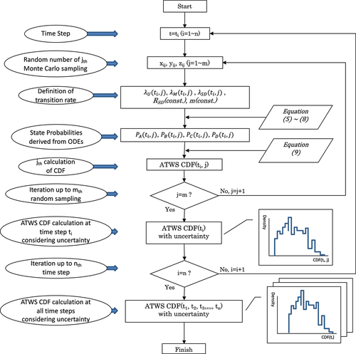
Based on these considerations, Figure 3 shows the computational flow of the uncertainty analysis of the CDF resulting from ATWS events due to the functional failure of DRPS proposed in this study.

Figure 3. A flow-chart showing uncertainty analysis process.

3.2. Case study

3.2.1. Analysis conditions and parameters

To demonstrate the applicability of the developed methodology, a case study was conducted using the proposed approach. In the case study, we defined the computational assumptions and parameters and performed numerical calculations using MATLAB®, a numerical analysis application, to determine the occurrence frequency and uncertainty of core damage due to ATWS (Anticipated Transient Without Scram) sequences.

While the basic analysis methodology follows the principles outlined in reference [21], the analysis conditions for this case study are as follows:

• Calculation terms involving time t from Equations (5)(5) $\frac{d{P}_A\left(t_i,\mathit{j}\right)}{\mathit{dt}}=\left\{-{\lambda }_M\left(t_i,\mathit{j}\right)-{\lambda }_U\left(t_i,\mathit{j}\right)\right\}\cdot P_A\left(t_i,\mathit{j}\right)+\left\{R_{\mathit{SD}}\cdot P_B\left(t_i,\mathit{j}\right)+\mathit{m}\cdot P_D\left(t_i,\mathit{j}\right)\right\},$(5)  ~ Equation (9)(9) ${\omega }_{C\hspace{0.17em}HF}^{\hspace{0.17em}}\left(t_i,\mathit{j}\right)={\lambda }_M\left(t_i,y_{\mathit{ij}}\right)\cdot P_C\left(t_i,\mathit{j}\right).$(9) consider the elapsed time from the start of any operation cycle.

• In this study, DRPS is assumed to have the surveillance tests. It is assumed that the detection efficiency of failures by the surveillance tests is perfect, and when a failure is detected, the assumed system, which is a single-channel configuration, immediately performs a manual shutdown operation with a transition rate ${\mu }_{\mathit{SD}}$, which puts the reactor into a shutdown state.

• The calculation period is assumed to be one year, corresponding to one operating cycle. After the start of operation, regular surveillance tests of DRPS are performed every 30 days. If DRPS is functioning properly, operation can continue after the surveillance tests. However, since the assumed DRPS is a single-channel configuration, if a failure occurs prior to the first surveillance test, a shutdown operation will be performed, resulting in a reactor shutdown state.

  In the case of the redundant system, the ability to continue operation for a period of time while repairing a single channel failure depends on the Limited Conditions of Operation (LCO) from the Tech Spec. As long as the remaining channel(s) are functioning properly according to the LCO, operation can continue until the repair is completed, except in cases where an automatic shutdown or manual shutdown is triggered by a demand occurrence.

• To compute the probabilities associated with each state at each time step, we use the system of simultaneous ordinary differential equations (ODEs) defined in Section II-3. We use the ODE23 solver in MATLAB® which uses the time step partitioning based on the rate of the change of state probabilities.

• It is assumed that a significant amount of time is required to transition from a reactor shutdown state to a normal operating state due to the preparations required for functional confirmation and restart. In this case, it is assumed to take 90 days. The transition rate for restart is the reciprocal of this time, i.e. the inverse of 90 days.

• Due to the significant challenges involved, the recovery of the plant after a core damage accident caused by an ATWS is considered to be practically almost impossible. Therefore, in this case, it is assumed to take an infinite amount of time (numerically approximated as 1 million hours). The transition rate for the recovery of the plant after the accident is the reciprocal of this time, i.e. the inverse of 1 million hours.

• Other conditions follow the descriptions in Section 2

Table 2 shows the parameters used in the case study. As mentioned earlier, the initial value of the probability P_A in the normal state is 1.0 at the beginning of the operating cycle, while the probabilities for all other states are set to 0. The numerical analysis of the system of simultaneous differential equations is performed using randomly sampled transition rates at each time step. The conditions related to the surveillance tests and the fault detection are specific to the periodic surveillance tests and are described as part of the MATLAB® script.

Table 2. List of parameters for case study.

Parameters	Measurements
λM(1/hr)	Mean=ln(1.0×10^−4)=-9.2,σ = 1.5
λU(1/hr)	Mean=ln(5.0×10^−8)=-16.8,σ = 2.5
μSD(1/hr)	Mean = 1, σ = 0.1 (After a surveillance test interval TS)
RSD(1/hr)	1/2160 as constant
m(1/hr)	∞(Defined as 1.0 × 10^−100) as constant

3.3. Results of the ATWS event frequency and EF

Based on the conditions and parameters described in the previous section, an analysis of the CDF and uncertainty following an ATWS event was performed. The changes with time in the probabilities of being in state A (Normal), state B (Shutdown), state C (DU Fault), and state D (Core Damage) are shown in Figures 4–7. While state D represents the core damage state, conventional PRA typically focuses on the frequency of occurrence of core damage rather than the probability of being in the core damage state. Therefore, using the concept described in Equation (9)(9) ${\omega }_{C\hspace{0.17em}HF}^{\hspace{0.17em}}\left(t_i,\mathit{j}\right)={\lambda }_M\left(t_i,y_{\mathit{ij}}\right)\cdot P_C\left(t_i,\mathit{j}\right).$(9) , the CDF is computed, and the result is shown in Figure 8 which shows the change with time in the CDF. Figures 4 through 7 show the mean, median, and upper and lower limits (95th and 5th percentiles) of the 90% confidence interval for the probabilities of being in states A through D, and Figure 8 shows those of the CDF.

Figure 4. State probabilities in the state a (normal).

Figure 5. State probabilities in the state B (shutdown).

Figure 6. State probabilities in the state C (DU fault).

Figure 7. State probabilities in the state D (ATWS).

Figure 8. CDF induced by ATWS.

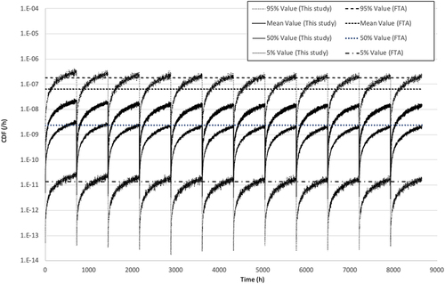
Figure 6 shows that the probability of being in state C is reset because the failure state is repaired by periodic functional verification tests performed every 720 hours, which is a particularly characteristic behavior. In this state, if a demand occurs, it will lead to ATWS and eventually core damage, so the CDF also shows the same behavior as the probability of being in state C. From Figure 8, the average of the mean value of the CDF between time 0 and 8640 (h) is 8.45E–9(/h), and the average of the EF (square root of the ratio between the 95th and 5th percentiles) is about 11.

These results demonstrate that it is possible to perform uncertainty analysis on the probabilities of each state and the CDF in the event of an ATWS incident caused by DRPS failure using the Markov state transition model. DRPS assumed in this study is not a redundant system, so if a failure is detected during the surveillance tests performed every 30 days in no-demand state, it will result in a manual shutdown. However, at the same time, all failure states are cleared and the computations show that the probability of being in state C (DU Fault) becomes zero (see Figure 6).

The CDF is calculated by multiplying the probability of being in state C by the occurrence rate of the demand. Therefore, the variability of the probability of being in state C and the variability of the occurrence rate of the demand amplify the variability of the CDF, resulting in noticeable fluctuations (see Figure 8). In addition, the Markov state transition model used in this study assumes that recovery from a core damage accident is almost impossible. It also assumes that it takes approximately three months to restart from state B (Shutdown). These assumptions create an environment similar to an absorbing Markov model. As a result, the probability of being in state A (Normal) gradually decreases.

As a result, the transition from state A (Normal) to state C (DU Fault) occurs based on the probability of being in state A. Therefore, as a general trend, the probability of being in state C (DU Fault) and the CDF gradually decrease. Conversely, the probability of being in state B (Shutdown) gradually increases. However, with the current parameter settings and the assumption of a non-redundant single-channel DRPS model in this study, the probabilities of being in state A (Normal) and state B (Shutdown) reach a kind of steady state with almost no change after 5000 hours.

The above interpretation provides a reasonable understanding of the results obtained from the case study conducted. It suggests that the analytical methodology used in this research allows the calculation of the CDF, including an appropriate uncertainty analysis.

3.4. Comparison with FTA technique

To demonstrate the validity of the developed methodology, a comparison is made between the results obtained using this method and those obtained using the Fault Tree Analysis (FTA) method and Monte Carlo calculations with random sampling of failure rates for uncertainty analysis of the CDF. In conventional L1PRA, fault trees and event trees are used to represent the logic of core damage. In this study, the target system DRPS is a single-channel system as shown in Figure 1. Therefore, the fault logic for core damage in the FTA can be represented by the superposition of a single channel fault (an undetectable fault: UD fault) and the occurrence of demands (an initiating event). Similar to the studies of Muta et al. [20] and Haruhara et al. [21], the sequence dependence is assumed such that the demand occurs under the occurrence of DRPS failures.

Therefore, the probability of occurrence of the UD failure in the conventional PRA method is calculated using the following equation:

$P_{\mathit{UD}\mathit{Fault}}={\lambda }_U\cdot T_S/2(11)$

Since the frequency of demand occurrence is expressed as the occurrence rate of demands, ${\lambda }_M$, the CDF F_CDF is calculated using the following equation. Note that the detection of failures during surveillance tests and subsequent repairs is difficult to account for in the FTA method and is not considered here.

$F_{\mathit{CDF}}=P_{\mathit{UD}\mathit{Fault}}\cdot {\lambda }_M={\lambda }_U\cdot T_S/2\cdot {\lambda }_M(12)$

Here, the failure rate ${\lambda }_U$and the occurrence rate of demands ${\lambda }_M$ remain constant. As mentioned in Chapter 3, the uncertainties of ${\lambda }_U$ and ${\lambda }_M$ are assumed to follow a log-normal distribution. They are defined by their respective mean and standard deviation, $\left({\mu }_{{\lambda }_U},{\sigma }_{{\lambda }_U}\right)$ and $\left({\mu }_{{\lambda }_M},{\sigma }_{{\lambda }_M}\right)$. Based on these probability density functions, random sampling is performed and the uncertainty of the CDF is calculated using Monte Carlo simulation.

Figure 8 shows the results of the analysis using the above models overlaid with the results of the uncertainty analysis method developed in this study. And Table 3 shows the comparison between the two methods. The EFs from this study are shown for every 720 hours and the average is shown at the bottom of the table. The EFs in this study varied slightly over time, but averaged 1.14E + 2, which is almost the same as the EFs from the conventional method.

Table 3. Comparison between the EFs of this study and those of the FTA.

Time (h)	EF (This Study)	EF (FTA)
1	1.13E + 02
720	1.08E + 02
1440	1.05E + 02
2160	1.02E + 02
2880	1.38E + 02
3600	1.16E + 02
4320	1.12E + 02
5040	1.05E + 02	1.14E + 02
5760	1.27E + 02
6480	1.07E + 02
7200	1.14E + 02
7920	1.16E + 02
8640	1.18E + 02
Average	1.14E + 02

Calculations based on the FTA method yield larger values for the mean, median, and upper/lower limits of the 90% confidence interval (95th percentile and 5th percentile) than those based on this method. This is because the FTA model cannot accurately represent the avoidance of core damage accidents through shutdown operations upon fault detection, resulting in a conservative evaluation.

However, it should be noted that although there are differences between the results of the uncertainty analysis using both methods, these differences can be explained, and the analysis method developed in this study is considered to be a more rigorous approach to the uncertainty analysis in the same context as the conventional FTA method. Therefore, it can be concluded that the analysis method of this study has developed into a more accurate method capable of performing uncertainty analysis. On the other hand, since this study focused on theoretical development using a DRPS model with the most basic configuration, there are aspects that need to be considered before applying this method in practical applications. These issues are discussed in the next chapter.

In addition, as an extension of the FTA method, there is a modeling method using order-dependent AND gates, which is also used for dynamic PRA. This method can be used to account for recovery prior to the occurrence of a demand, but even for the simple system considered here, it is difficult to model all possible event sequences because the model becomes too complex and it is difficult to handle changes in state probabilities over time. This is considered to be difficult in practice. The method of this study is significant in that it is relatively easy to model with a Markov state transition model and simultaneous differential equations describing the state transitions.

3.4.1. Treatment of state transition including dd fault and s/w fault

In this study, we have focused on developing a methodology using the example of the state transition of a DRPS, specifically targeting DU faults that can be detected by periodic surveillance tests rather than continuous monitoring. The basis of the development methodology in this study is derived from the works of Muta et al. [20] and Haruhara et al. [21], which also consider DD faults that can be immediately detected by continuous monitoring, as well as software failures that control digital circuits. If these faults are also part of a single-channel configuration and require a shutdown operation upon detection, the methodology developed in this study can generally be applied without significant modifications.

Furthermore, in the case of redundant systems, such as the 1 out of 2 configuration shown in Figure 9 of reference [21], the main state transitions are expected to be similar to those in the state transition model developed in this study, but there are additional considerations in redundant systems that were not considered in this study. These include the possibility of repair in the case of a single channel failure, the possibility of repair or the need for shutdown in the case of multiple channel failures, and the continuation of operation after successful repair, which are described in reference [21]. Therefore, by using Equations (1)(1) $\frac{d{P}_A}{\mathit{dt}}=\left\{-{\lambda }_M-{\lambda }_U\right\}\cdot P_A+\left\{R_{\mathit{SD}}\cdot P_B+\mathit{m}\cdot P_D\right\},$(1) to Equation (9)(9) ${\omega }_{C\hspace{0.17em}HF}^{\hspace{0.17em}}\left(t_i,\mathit{j}\right)={\lambda }_M\left(t_i,y_{\mathit{ij}}\right)\cdot P_C\left(t_i,\mathit{j}\right).$(9) in reference [21] and the ideas presented in Section II.3 of this study, uncertainty analysis of redundant systems with 1 out of 2 configurations can be performed.

Figure 9. A state-transition diagram of core damage event (1 out of 2 configuration).

Furthermore, by applying the random numbers given in Table 4 and the parameters given in Table 5, the results of the uncertainty analysis shown in Figure 10 can be obtained as an example. This case study clearly demonstrates the applicability of the methodology of this study to the redundant system.

Figure 10. CDF induced by ATWS (1 out of 2 configuration).

Table 4. Summary of the treatment of the random sampling for 1 out of 2 configuration.

Parameters	Treatment of random sampling
vij for λD(ti, j)	Using same random number regardless of time step
wij for μD(ti, j)	Using different random numbers depending on time step
uij for μU(ti, j)	Using different random numbers depending on time step
rij for μSDDD(ti, j)	Using different random numbers depending on time step

*:$x_{\mathit{ij}}$ for ${\lambda }_U\left(t_i,\mathit{j}\right)$, $y_{\mathit{ij}}$ for ${\lambda }_M\left(t_i,\mathit{j}\right)$, $z_{\mathit{ij}}$ for ${\mu }_{\mathit{SD}}\left(t_i,\mathit{j}\right)$, R_SD and m are treated in a same manner as Table 1.

Table 5. List of parameters for case study (1 out of 2 configuration).

Parameters	Measurements
λM(1/hr)	Mean=ln(1.0×10^−4)=-9.2,σ = 1.5
λU(1/hr)	Mean=ln(5.0×10^−8)=-16.8,σ = 2.5
λD(1/hr)	Mean=ln(4.95×10^−6)=-12.2,σ = 1.5
μD(1/hr)	Mean = 0.1, σ = 0.1 (After a surveillance test interval TS)
μU(1/hr)	Mean = 0.1, σ = 0.1 (After a surveillance test interval TS)
μSD(1/hr)	Mean = 0.5, σ = 0.1 (After a surveillance test interval TS)
μSDDD(1/hr)	Mean = 0.5, σ = 0.1 (After a surveillance test interval TS)
RSD(1/hr)	1/2160 as constant
m(1/hr)	∞(Defined as 1.0 × 10^−100) as constant

In addition to multiple independent failures and software failures, common cause failures must also be considered in redundant systems. In principle, the concepts and methodology developed in this study can be applied to these scenarios as well. However, the specific application of the methodology to these cases is left as a future task to be addressed in future work.

4. Conclusion

The modeling of DRPS in conventional PRA has been considered challenging. However, the authors have developed a methodology based on the use of Markov state transition models, using both static and dynamic approaches. Based on these previous studies, this study has developed a methodology to analyze the uncertainty in the frequency of ATWS events, considering the time dependence.

The methodology proposed in this study allows the CDF evaluation and uncertainty analysis considering the state transitions of DRPSs, which are difficult to model using conventional FTA methods. Regarding the applicability of the proposed methodology to DRPSs with redundant systems, it is shown that the possible state transitions in DRPSs can be modeled, and that quantitative evaluation and uncertainty analysis of the CDF can be performed. Conventional methods have difficulty in handling the characteristic state transitions of DRPSs, such as fault self-diagnosis, repair from fault states, and manual shutdown operation when a fault is detected, and therefore uncertainty analysis based on an appropriate reliability analysis model has not been possible. The proposed methodology consists of a Markov state transition model, simultaneous differential equations describing the state transitions, and a Monte Carlo-based uncertainty analysis method. It is considered to be more practical than conventional methods.

This methodology is consistent with the that of conventional PRA, allowing uncertainties to be analyzed in a compatible manner. The dynamic approach using Markov state transition models allows the analytical consideration of all state transitions, eliminating the excessive conservatism resulting from the omission of factors such as shutdown operations.

As mentioned in the previous study [21], it is not possible to model non-Markovian state transitions with the methodology of this study, such as human error including failures in shutdown operations. However, there is a possibility to incorporate such state transitions by integrating them with the conventional FTA method. The specific methodology to accomplish this study remains a future task and requires further study.

In the future, as mentioned above, further considerations are needed to apply this methodology to more practical PRA scenarios. These considerations include extending the coverage of failure modes, modeling continuous monitoring and functional testing, applying to highly redundant systems that resemble actual installations, and exploring methodologies to achieve practical computational accuracy and efficiency. The study of these aspects has already begun and will contribute to the application of this methodology in practical PRA.

Acknowledgments

The authors would like to thank the members of the Nuclear Risk Assessment Laboratory at Tokyo City University for their helpful support in these successive studies, as well as anonymous referees for their helpful comments.

Disclosure statement

No potential conflict of interest was reported by the authors.

References

- Nuclear Regulation Authority, Operational guidelines for Enhancing the safety of practical Power Reactors, Mar. 2020. [in Japanese]
- Nuclear Power Engineering Corporation (NUPEC). “The report of establishment of Level 1 PSA method of ABWR plant at Power operation (1998), Japan: Nuclear Power Engineering Corporation; 1999. INS/M98–26. [in Japanese]
- Japan Nuclear Energy Safety Organization (JNES). “The report of establishment of Level 1 PSA method for PWR plants at Power operation = 3-loop PWR plant with/without accident Management Countermeasures=,” Japan: Japan Nuclear Energy Safety Organization; 2009, JNES/SAE08–013. [in Japanese]
- U.S.NRC. Dynamic reliability modeling of digital Instrumentation and control systems for Nuclear reactor probabilistic risk assessments (NUREG/CR-6942). U.S.NRC; Oct 2007.
- U.S.NRC. Traditional probabilistic risk Assessment methods for digital systems (NUREG/CR-6962). U.S.NRC; Oct 2008.
- U.S.NRC, A benchmark implementation of two dynamic methodologies for the reliability modeling of digital Instrumentation and control systems (NUREG/CR-6985), Sept. 2009.
- U.S.NRC. Development of a statistical testing approach for quantifying safety-related digital system on demand failure probability (NUREG/CR-7234). U.S.NRC; Dec 2017.
- Torkey H, Saber AS, Shaat MK, et al. Bayesian belief-based model for reliability improvement of the digital reactor protection system. Nucl Sci Tech. 2020 [Oct. 2020];31(10):101. doi: 10.1007/s41365-020-00814-6
- U.S.NRC. Developing a Bayesian belief network model for quantifying the probability of software failure of a protection system (NUREG/CR-7233). U.S.NRC; Jan 2018.
- Seop Son K, Kim DH, Kim CH, et al. Study on the systematic approach of Markov modeling for dependability analysis of complex fault-tolerant features with voting logics. Reliab Eng Syst Saf. 2016 [Feb. 2016];150:44–57.
- Bulba Y, et al. Classification and research of the reactor protection instrumentation and control system functional safety Markov models in anormal operation Mode . Proceedings of the 12th International Conference on ICT in Education, Research and Industrial Applications: Integration, Harmonization and Knowledge Transfer; 2016 June 21-24; Kyiv: Ukraine.
- Nuclear Power Engineering Corporation (NUPEC). “The report of establishment of Level 1 PSA method of ABWR plant at Power operation (1999),” Japan: Nuclear Power Engineering Corporation; 2000, INS/M99–29. [in Japanese]
- Nuclear Power Engineering Corporation (NUPEC). “The report of establishment of Level 1 PSA method for internal events at Power operation = reliability analysis of digital reactor protection system = (2002) Japan: Nuclear Power Engineering Corporation; INS/M02–29. [in Japanese]
- Japan Nuclear Energy Safety Organization (JNES). “The report of establishment of Level 1 PSA method for internal events at Power operation = improvement of reliability analysis of digital reactor protection system (PWR) =,” Japan: Japan Nuclear Energy Safety Organization; 2007, JNES/SAE07–029. [in Japanese]
- Authen S, Holmberg JE. Reliability analysis of digital systems in a probabilistic risk analysis for Nuclear Power plants. Nucl Eng Technol. 2012 June;44(5):471–482. doi: 10.5516/NET.03.2012.707
- Piljugin E, Authén S, Holmberg JE. “Proposal for the taxonomy of failure modes of digital system hardware for PSA,” 11th International Probabilistic Safety Assessment and Management Conference & The Annual European Safety and Reliability Conference; 2012 June; Helsinki, Finland. [ CD-ROM]
- Chu TL, Yue M, Postma W. “A Summary of taxonomies of digital system failure modes provided by the DigRel task group.” 11th International Probabilistic Safety Assessment and Management Conference & The Annual European Safety and Reliability Conference; 2012 June; Helsinki, Finland. [ CD-ROM]
- Muta H, Muramatsu K. Quantitative modeling of digital reactor protection system using Markov state-transition model. J Nucl Sci Technol. 2014;51(9):1073–1086. doi: 10.1080/00223131.2014.906331
- Muta H. Application of Markov state-transition model to reliability analysis of 2-out-of-4 reactor trip system. Trans At Energy Soc Jpn. 2015;14(1):25–39. doi: 10.3327/taesj.J14.011
- MUTA H, FURUYA O, MURAMATSU K. Proposal of PRA methodology considering state transitions and time-dependent failure rates of components. Transactions Of The Atomic Energy Society Of Japan. 2016;15(2):70–83. doi: 10.3327/taesj.J15.004
- HARUHARA M, MUTA H, Ohtori Y et al. Proposal of quantification method of dynamic system reliability model of digital RPS using Markov state-transition model. Journal Of Nuclear Science And Technology. 2023 Feb;60(9):1154–1167. doi: 10.1080/00223131.2023.2169379
- U.S.NRC. Guidance on the Treatment of uncertainties associated with PRAs in risk-informed decision making, final report (NUREG-1855, revision 1). U.S.NRC; Mar 2017.
- Atomic Energy Society of Japan. A standard for Procedures of probabilistic safety Assessment of Nuclear Power plants during Power operation. Japanese: AESJ; 2022.
- OECD/NEA/CSNI Failure modes taxonomy for reliability Assessment of digital Instrumentation and control systems for probabilistic Risk analysis. OECD/NEA/CSNI/R; 2014.