Multilevel process monitoring: A case study to predict student success or failure

Abstract

In this case study, we demonstrate the use of multilevel process monitoring in quality control. Using high school data, we answer three research questions related to high school student progress during an academic year. The questions are (1) What determines student performance? (2) How can statistical process monitoring be used in monitoring student progress? (3) What method can be used for predictive monitoring of student results? To answer these questions, we worked together with a Dutch high school and combined hierarchical Bayesian modeling with statistical and predictive monitoring procedures. The results give a clear blueprint for student progress monitoring.

Keywords:

• hierarchical Bayesian
• multilevel
• predictive monitoring
• statistical process monitoring
• student performance

1. Motivation

“Early Warning Indicator Reports were invaluable to the success of our school” (high school principal, a quote from the Strategic Data Project Report by Becker et al. (2014)). These early warning indicator reports monitor students throughout their school career and warn teachers and staff of students with high dropout risks. According to Romero and Ventura (2019), such early identification of vulnerable students who are prone to fail or drop their courses is crucial for the success of any learning method. Also, monitoring allows for the identification of students who are insufficiently challenged and will benefit from more stimulating classroom material.

Navigating the large body of literature in statistical process monitoring, predictive monitoring and educational data mining is a daunting task when looking for answers as to what metrics should be monitored and which methods should be implemented.

Multilevel modeling is often a good method in educational settings and can be used for predictive monitoring in quality control. In this article, we demonstrate such a procedure and aim to guide researchers and practitioners in monitoring student performance, specifically in a high school setting. To achieve this, we work closely with a Dutch high school to answer the following questions 1) What determines student performance? 2) How can statistical process monitoring be used in monitoring student progress? 3) What method can be used for predictive monitoring of student results?

1.1. Statistical process monitoring

Statistical process monitoring (SPM) provides techniques to monitor a process real time. As the amount and complexity of available data are increasing, there is a need for SPM methods that utilize more of the inherent structure of the data. This need has driven SPM to evolve in recent years from univariate methods monitoring a single quality indicator, to monitoring methods for complex multivariate processes. A method that is used for multivariate processes are profile monitoring. Profile monitoring checks the stability of the modeled relationship between a response variable and one or more explanatory variables over time. Often profile monitoring uses regression control charts which were first introduced by Mandel (1969). The current body of regression control charting literature almost exclusively handles the monitoring of linear profiles using classical regression models. Weese et al. (2016) noted that large data sets often contain complex relationships and patterns over time, such as hierarchical structures and autocorrelation.

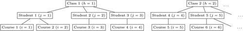
The case study presented in this paper contains complex relationships and patterns, notably the hierarchical structure of courses, students and classes (see Figure 1). State-of-the-art multivariate control charting based on linear regression models ignores this structure. However, incorporating hierarchical structures into the models can improve the reliability of a monitoring system. Therefore, we will develop a control chart that can signal at three levels, the class, student and course level. Also, Woodall and Montgomery (2014) gave an overview of current directions in SPM and highlighted profile monitoring with multiple profiles per group as a topic for further research.

Figure 1. The hierarchical structure of the case study data with classes as the top level. Students within these classes are the middle level and courses followed by these students form the lower level.

The advantage of using a hierarchical model is an improved estimation of process variability; according to Gelman (2006), hierarchical modeling is almost always an improvement compared to classical regression. The reason is that a hierarchical model includes the effects of both observed and unobserved variables, where unobserved variables are not explicitly measured but inherent to the group. Another advantage over classical regression is that a multilevel model provides a way to monitor new groups since the model generates some prior beliefs upon which to base the distribution and the prediction for the new groups. Furthermore, in contrast with classical regression, multilevel modeling is capable of prediction for groups with a small number of observations.

Multilevel models have been used in agricultural and educational applications for decades (Henderson et al. 1959; Aitkin and Longford 1986; Bock 1989; Aaronson 1998; Sellström and Bremberg 2006). Today, hierarchical models are used in spatial data modeling (Banerjee, Carlin, and Gelfand 2014), extreme value modeling (Sang and Gelfand 2009), quantum mechanics (Berendsen 2007) and even in the modeling of intimacy in marriage (Laurenceau, Barrett, and Rovine 2005). However, to the best of our knowledge, multilevel modeling has not found its way to SPM. Schirru, Pampuri, and De Nicolao (2010) modeled multistream processes in semiconductor manufacturing using a multilevel model, but it is only applicable to two levels. Qiu, Zou, and Wang (2010) considered nonparametric profile monitoring using mixed-effects modeling, although they did not consider hierarchical modeling.

This article will explore process monitoring for a school data set that contains the grades of students in different groups over time. The school is interested in monitoring deviations in student results from what is given by the model, which is a form of profile monitoring. Therefore, we will investigate SPM based on hierarchical Bayesian models. In the next section, we will discuss the use of a hierarchical model to predict outlying results on the student level.

1.2. Predictive monitoring

Becker et al. (2014) emphasized the need for actionable predictive analytics in high schools to keep students on track toward graduation and better prepare them for college and career success. The report discussed three examples of early warning indicator systems that help school teachers and management with early identification of students with a lower probability of passing, based on logistic regressions of student grade and attendance information.

Early prediction of learning performance has gained more traction in the literature, as showcased by a recent special issue of IEEE Transactions on learning technologies. Together with monitoring big and complex data, predictive monitoring is recently being considered in quality technology literature (for example Kang et al. 2018; Wang et al. 2019). Although our case study focuses on the use of predictive monitoring to improve the quality of education, the presented methods can be used in any setting where clear hierarchical data structures exist. Baghdadi et al. (2019) stated that the ability to estimate when the performance will deteriorate and what type of intervention optimizes recovery can improve the quality and productivity and reduce risk concerning worker fatigue. Our case study offers a very similar approach to improve the quality and productivity of high school education by monitoring student performance.

The hierarchical model will thus be applied in two ways. First, control charting is applied based on the multilevel model. Second, the multilevel model is used for predicting results on the student level. This results in a hierarchical early warning indicator system that can be applied in schools for predictive monitoring of student outcomes.

The outline of this paper is as follows. The next section describes the relevant educational literature, the practical problem we aim to solve and the data that was available. The hierarchical model and its performance are discussed in the section after this, followed by a section that investigates student performance monitoring. The last section summarizes the results.

2. Problem description

In this section, we describe related student performance literature, the goal of the method to be developed and the data set including the predictor variables.

2.1. Student performance literature

This section will shortly discuss a selection of determinants of student performance, whose selection has been based on a literature study. The determinants, their expected effects on performance and their modeling approach are summarized in Table 1. The important variables will be used in the modeling approaches of later sections. The “unobserved” variables represent variables that were not available in this study, but the hierarchical modeling specification incorporates many of these “unobserved differences” between students and students within courses.

Table 1. Summary of determinants of student performance according to the literature and modeling approach.

Determinant	Effect on performance
	Student level	Class level	Modeling approach
SES		+	Explanatory variable
Disabilities	–		Explanatory variable
Language	+/–		Explanatory variable
Non-native	+/–	–	Explanatory variable
Student effort	+	+	Student unobserved heterogeneity
Peer associations	+/–	+/–	Student/course unobserved heterogeneity
Parent involvement	+		Student unobserved heterogeneity
School climate	+/–	+/–	Course unobserved heterogeneity
Intelligence	+		Explanatory variable, student unobserved heterogeneity
Grades	+		Time varying explanatory/dependent variable
Absences	–	–	Time varying explanatory variable

Nichols (2003) found a significant relationship between poor performance at the beginning of students’ educational careers and later on. Furthermore, students who struggle academically had increased school absences and students from lower-income families showed a higher probability of poor results. This suggests an important role for family income, absences and temporal effects in predicting individual high school performance.

Socioeconomic status (SES) has long been argued to significantly affect school performance, although the importance varies greatly among different analyses. Geiser and Santelices (2007) argued omission of socioeconomic background factors can lead to significant overestimation of the predictive power of academic variables, that are strongly correlated with socioeconomic advantage. They based this assumption on a study by Rothstein (2004), which argued the exclusion of student background characteristics from prediction models inflates college admission tests’ apparent validity by over 150 percent.

Disabilities can be a determinant of student performance. Dyslexic children fail to achieve school grades at a level that is commensurate with their intelligence (Karande and Kulkarni 2005). Although they might not be directly linked to learning, disabilities like asthma, epilepsy, and autism can indirectly influence academic performance. Autistic children can face a lot of problems in school as their core features impair learning. Furthermore, medical problems like visual impairment, hearing impairment, malnutrition, and low birth weight can cause difficulties in school.

The language that children speak at home can influence their academic abilities both positively (Buriel et al. 1998) and negatively (Kennedy and Park 1994). Collier (1995) found that immigrants and language minority students need 4–12 years of second language development for the most advantaged students to reach deep academic proficiency and compete successfully with native speakers. It has been suggested that the presence of non-native speakers in schools harms the performance of native speakers, but this has been refuted by Geay, McNally, and Telhaj (2013). In contrast, children who interpret for their immigrant parents; “language brokers,” often perform better academically (Buriel et al. 1998).

Some variables remain unobserved but can be incorporated in models by allowing for unobserved heterogeneity. One is student effort, which is characterized by the level of school attachment, involvement, and commitment displayed by the student (Stewart 2008). Also, peer influence, i.e. the associations between high school students, matter a great deal to individual academic achievement and development (Nichols and White 2001). Besides, parent involvement is likely to influence academic achievement. Sui-Chu and Willms (1996) found that the most important dimension of parent involvement toward academic achievement is home discussion. They suggested facilitating home discussion by providing concrete information to the parents about parenting styles, teaching methods, and school curricula. Finally, school climate (a.o. Stewart 2008) and intelligence (Rohde and Thompson 2007; Laidra, Pullmann, and Allik 2007; Parker et al. 2006) are important for academic achievement.

Parent involvement, disciplinary climate, and individual intelligence are usually quite difficult to measure. This study aims to incorporate them nonetheless. Parent involvement is incorporated mostly in student unobserved heterogeneity. Limited observed information on the parents is included in the predictive model (i.e. education level and SES). Disciplinary climate and class disruptions are mostly covered by including absences that equate to dismissals from class and within unobserved course differences. Individual intelligence is approximated using primary school test scores.

Next, some time-varying variables are important. The first variable is the grade. For each course, specific tests are taken with varying weights. Anytime during the year, these tests determine a current weighted average grade for each student and course. The resulting end-of-year grade is the most important student performance indicator. Also, absences are important as attending class helps students understand the material and motivates their participation (Rothman 2001). The variables test grades and absences are generated over time. Finally, temporal effects on student performance encompass both inter-year changes and intra-year changes. Students will change the allocation of their effort and time according to their current average grade, their average grade for other courses, seasonal effects, within school changes and external factors. Ideally, modeling will allow for student and course-specific effects to vary over time. The next section will describe the Dutch high school system.

2.2. The Dutch high school system

The Dutch school system in general consists of eight years of primary school, followed by four, five or six years of high school. There is one level of primary school, but there are multiple levels of high school. Two criteria have been used in recent years to determine the level of high school a child is allowed to go to. Firstly, there is the teacher’s advice. The teacher advises the level that fits the child in the final year of primary school. This advice is based on the performance of the child in a specific primary school.

Secondly, the National Institute for Test Development (in Dutch: Centraal Instituut voor Toets Ontwikkeling, abbreviated by CITO) test is a test that is developed by the CITO organization and is scientifically designed to test a child’s academic abilities. It was initiated in the Netherlands by the famous psychologist professor A.D. de Groot in 1966 and every school is required to conduct the CITO or a similar test at the end of primary school as of 2014.

To pass any specific year of high school, conditions set by the school have to be met. These conditions usually consist of requirements on the end-of-year average grades for all the student’s courses. The grades in most Dutch high schools are on a scale of 1 to 10. The end-of-year grades are usually rounded, and a course is failed or “insufficient” if the rounded grade is below 6. The amount of allowed “failpoints,” i.e. the total points below six, can then be restricted. A school might, for example, have a student repeat the current year if he or she scores more than two failpoints, which could be a student with a grade of three for a single course, or a four and a five or three fives at the end of the year. The restrictions are not limited to the number of failpoints. There can be requirements on the total average grade and certain subtleties emerge once the students start splitting up into high school profiles, where different students do a different set of courses from their fourth year on. These school profiles can have special requirements, with usually more importance assigned to the profile courses.

When implementing a predictive monitoring scheme in a school, the specific rules a school employs define the passing probability that is estimated. When for example a student is failing a profile course, this can lead to failing the year directly. If the same student would obtain the same grade for a different course, this would not necessarily mean failing the year. Therefore, different courses have different levels of importance to the probability of success for individual students. The school that has kindly provided the data described in the next section has different passing conditions for each year. Although the implementation at the school incorporates all conditions, the predictive analyses in this paper reflect a simplified version to demonstrate the detective capabilities of the methods.

2.3. Data set

A large, detailed data set was provided by a Dutch high school. In total there are eight years of data available, comprising of 36 different subjects followed by over 1,700 unique students (about 51% girls) and 711,653 individual tests. The students were born in 38 different countries, speak 18 different languages and were taught by 110 different teachers. Out of the unique students, 326 had some kind of disability while at school, 162 had a non-Dutch nationality and 51 students had a serious language barrier. The number of students with parents who have attended university or higher-level academics is 261 and 86% of students were residents of the large city that the school is located in during their time at the Dutch high school.

To incorporate socioeconomic status (SES) in this analysis, nation-wide social status data provided by the Dutch government was used. The relative SES score of a student using a country-wide ranking of his or her postal code was added to the data set.

Learning disabilities that have been confirmed by the school are included in the data set. The most common learning disabilities in the data are Attention-Deficit/Hyperactivity Disorder (ADHD) and dyslexia.

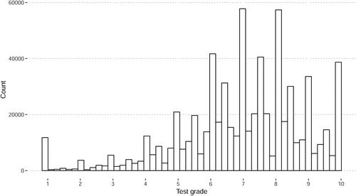
The data used in this paper contains grades that are on a 1-10 scale. Although easy to interpret, there arise some difficulties when using these grades for modeling. First, as Figure 2 shows, there are peaks at integer grades and grades on a.5 scale. This is due to teachers grading on an integer or.5 point scale instead of using continuous grades. This becomes less of a problem with average grades, as they are eventually rounded but fairly continuous during the year.

Figure 2. Histogram of the individual test grades in the data.

Second, when predicting the precise end-of-year grade, grades below 1 or above 10 should be impossible. However, both grades should have some positive probability, as some students do achieve average grades of 10 for specific courses during a year.

The following section describes the selected predictor variables in the data.

2.4. Determinants of student performance

We have discussed some of the literature on determinants of high school performance in Section 2.1. This section investigates these variables in the data.

The raw values for the most important categorical variables in the data are plotted in Figure 3. The first pair of boxplots in Figure 3 shows that girls seem to outperform boys in terms of final grades, which is consistent with the literature in different settings (see Rahafar et al. 2016; Deary et al. 2007; Battin-Pearson et al. 2000 for examples of gender gap findings in academic achievement). The second pair of boxplots in Figure 3 indicates that students with a disability achieve lower end-of-year grades, consistent with the findings of Karande and Kulkarni (2005). Children of highly educated parents seem to perform slightly better at this school in terms of final grades, as depicted in the third pair of boxplots in Figure 3.

Figure 3. Boxplots of the final grades for the most important categorical predictor variables.

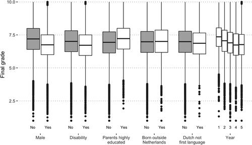
In line with Buriel et al. (1998), children born outside of the Netherlands do not underperform as shown by the fourth pair of boxplots in Figure 3. Students with a different native language do achieve slightly lower grades in the data, supporting conclusions by Collier (1995) and Kennedy and Park (1994). The end-of-year grades are lower toward the end of high school, as indicated in Figure 3.

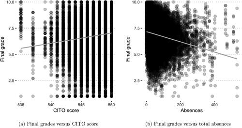
Figure 4 shows the two most important numerical independent variables plotted against the final grades. The CITO score has a positive correlation with grades as shown by the positive linear trend in Figure 4a. This makes sense, as the CITO test is designed as a predictor of individual intelligence. Furthermore, in line with Rothman (2001), more absences mean lower final grades in the data, as indicated by the negative linear trend in Figure 4b.

Figure 4. Scatterplots of the final grades and most important numerical variables with a linear trend-line.

3. Hierarchical model

The objective is to monitor student progress during the school year, where the school’s main interest lies in signaling “exceptional” students. Exceptional students can be both underperforming and overperforming students. In this section, we introduce a three-level hierarchical model for student grades and compare its performance to simpler models in monitoring student performance.

3.1. The model

Throughout the year, students take tests for every course $i=1,\dots .,n_0.$ The grades for these tests are defined as $g_{ki}\in [1,10]$ with $k=1,..,K_i,$ where K_i is the number of tests taken in course i. As these grades are obtained for individual tests, we have a set of cumulative weighted average grades $y_{i,j[i],h[j[i]]}$ for course i, student j and class h. For readability we drop subscripts j and h. The individual test results g_ki and the weights of the tests w_ki determine the average grade $y_i=\frac{{\sum }_{k=1}^{K_i}{w}_{ki}{g}_{ki}}{{\sum }_{k=1}^{K_i}{w}_{ki}},$ with $y_i\in [1,10].$

We consider a hierarchical model with three levels and use the index $i(i=1,2,\dots ,n_0)$ to denote the individual course level, $j(j=1,2,\dots ,n_1)$ to denote the individual student level and $h(h=1,2,\dots ,n_2)$ for the class level (see Figure 1). We have p₀ predictors for the course level, p₁ for the student level and p₂ for the class level. We define row vectors ${\mathit{X}}_{\mathit{i}}^{({\mathit{L}}_{\mathbf{0}})},{\mathit{X}}_{\mathit{j}}^{({\mathit{L}}_{\mathbf{1}})}$ and ${\mathit{X}}_{\mathit{h}}^{({\mathit{L}}_{\mathbf{2}})},$ which consist of the intercept and predictor values for the course, student and class levels respectively.

We model cumulative weighted average grade y_i for course i as $$y_i\sim N({\mathit{X}}_{\mathit{i}}^{({\mathit{L}}_{\mathbf{0}})}{\mathit{\beta }}_{\mathit{j}\left[\mathit{i}\right]}^{({\mathit{L}}_{\mathbf{0}})},{\sigma }^2),\mathrm{ }\text{for}\mathrm{ }i=1,\dots ,n_0\mathrm{ }\mathrm{(}\text{Course}\mathrm{ }\text{level}\mathrm{)},$$ where the student levels are modeled as $${\mathit{\beta }}_{\mathit{j}}^{({\mathit{L}}_{\mathbf{0}})}\sim N({\mathit{\beta }}_{\mathit{h}\left[\mathit{j}\right]}^{({\mathit{L}}_{\mathbf{1}})}{\mathit{X}}_{\mathit{j}}^{({\mathit{L}}_{\mathbf{1}})\prime },{\mathbf{\Sigma }}^{({\mathit{L}}_{\mathbf{1}})}),\mathrm{ }\text{for}\mathrm{ }j=1,\dots ,n_1\mathrm{ }\mathrm{(}\text{Student}\mathrm{ }\text{level}\mathrm{)},$$ and the class levels are specified by $$\mathit{vec}({\mathit{\beta }}_{\mathit{h}}^{({\mathit{L}}_{\mathbf{1}})})\sim N({\mathit{\beta }}^{({\mathit{L}}_{\mathbf{2}})}{\mathit{X}}_{\mathit{h}}^{({\mathit{L}}_{\mathbf{2}})\prime },{\mathbf{\Sigma }}^{({\mathit{L}}_{\mathbf{2}})}),\mathrm{ }\text{for}\mathrm{ }h=1,\dots ,n_2\mathrm{ }\mathrm{(}\text{Class}\mathrm{ }\text{level}\mathrm{)},$$ where ${\mathit{X}}_{\mathit{i}}^{({\mathit{L}}_{\mathbf{0}})}$ is a $1\times (p_0+1)$ row vector of subject specific variables such as course content and level; ${\mathit{\beta }}_{\mathit{j}[\mathit{i}]}^{({\mathit{L}}_{\mathbf{0}})}$ is a $(p_0+1)\times 1$ vector of parameters for student j that follows course i; ${\sigma }^2$ is the variance for the course level; ${\mathit{\beta }}_{\mathit{h}[\mathit{j}]}^{({\mathit{L}}_{\mathbf{1}})}$ is a $(p_0+1)\times (p_1+1)$ parameter matrix determined by the class h that student j is in; ${\mathit{X}}_j^{(L_1)}$ is a $1\times (p_1+1)$ row vector of student specific variables such as age, absences and IQ; ${\mathbf{\Sigma }}^{({\mathit{L}}_{\mathbf{1}})}$ is the covariance matrix for parameters ${\mathit{\beta }}_{\mathit{j}}^{({\mathit{L}}_{\mathbf{0}})};$ $\mathit{vec}({\mathit{\beta }}_{\mathit{h}}^{({\mathit{L}}_{\mathit{1}})})$ is the vectorized version of ${\mathit{\beta }}_{\mathit{h}}^{({\mathit{L}}_{\mathbf{1}})}$ with dimensions $(p_0+1)(p_1+1)\times 1;$ ${\mathit{\beta }}^{({\mathit{L}}_{\mathbf{2}})}$ is a $(p_0+1)(p_1+1)\times (p_2+1)$ parameter matrix at the class level; ${\mathit{X}}_h^{(L_2)}$ is a $1\times (p_2+1)$ row vector of class specific variables such as class size; and ${\mathbf{\Sigma }}^{({\mathit{L}}_{\mathbf{2}})}$ is the covariance matrix for parameters ${\mathit{\beta }}_{\mathit{h}}^{({\mathit{L}}_{\mathbf{1}})}.$

3.2. Estimation

The parameters of a multilevel model can be estimated using, among other methods, maximum likelihood, generalized least squares and Bayesian theory (Hox, Moerbeek, and Van de Schoot 2017). A discussion of Bayesian and likelihood-based techniques for multilevel models is given by Browne and Draper (2006). These authors show that Bayesian estimation often provides an improvement over likelihood methods in terms of both point and interval estimates as well as the posterior distributions for the parameters. We use Bayesian estimation to estimate the parameters in this article.

The full parameter space $\{{\mathit{\beta }}^{({\mathit{L}}_{\mathbf{0}})},{\sigma }^2,{\mathit{\beta }}^{({\mathit{L}}_{\mathbf{1}})},{\mathbf{\Sigma }}^{({\mathit{L}}_{\mathbf{1}}),{\beta }^{(L_2)},{\Sigma }^{(L_2)}}\},$ where ${\mathit{\beta }}^{({\mathit{L}}_{\mathbf{0}})}$ and ${\mathit{\beta }}^{({\mathit{L}}_{\mathbf{1}})}$ are constructed by stacking the parameter matrices ${\mathit{\beta }}_{\mathit{j}}^{({\mathit{L}}_{\mathbf{0}})}$ and ${\mathit{\beta }}_{\mathit{h}}^{({\mathit{L}}_{\mathbf{1}})}$ for all groups j and h respectively, can be estimated based on data that are considered representative, i.e. in control. To estimate the parameters, we use the Bayesian method applying Markov Chain Monte Carlo (MCMC) methods which use the Gibbs sampling procedure. These methods are described in the appendix and are applied using the rJAGS package to link to JAGS (Plummer 2018).

As the number of parameters increases quickly with added group levels, estimation time increases greatly as well. Thus when defining a multilevel model, there is a tradeoff between added precision and the additional estimation time for a group level. In a two-level model, the number of parameters we need to estimate is 1 for ${\sigma }^2,(p_0+1)(p_1+1)$ for ${\mathit{\beta }}^{({\mathit{L}}_{\mathbf{1}})}$ and $\frac{1}{2}(p_0+1)(p_0+2)$ for ${\mathbf{\Sigma }}^{({\mathit{L}}_{\mathbf{1}})}$ (${\mathit{\beta }}^{({\mathit{L}}_{\mathbf{0}})}$ is constructed using the estimates for ${\mathit{\beta }}^{({\mathit{L}}_{\mathbf{1}})}$). For the three-level model this increases, with 1 for ${\sigma }^2,\frac{1}{2}(p_0+1)(p_0+2)$ for ${\mathbf{\Sigma }}^{({\mathit{L}}_{\mathbf{1}})},(p_0+1)(p_1+1)(p_2+1)$ for ${\mathit{\beta }}^{({\mathit{L}}_{\mathbf{2}})}$ and $\frac{1}{2}(p_0+1)(p_1+1)((p_0+1)(p_1+1)+1)$ for ${\mathbf{\Sigma }}^{({\mathit{L}}_{\mathbf{2}})}$ (${\mathit{\beta }}^{({\mathit{L}}_{\mathbf{0}})}$ and ${\mathit{\beta }}^{({\mathit{L}}_{\mathbf{1}})}$ are constructed using the estimates for ${\mathit{\beta }}^{({\mathit{L}}_{\mathbf{2}})}$). For example, if there are three parameters per level, the number of parameters is 27 for a two-level model and 211 for a three-level model.

After applying the estimation procedure as described in the appendix, we obtain the estimations for the parameters in the three-level model, which we denote by $\{{\widehat{\mathit{\beta }}}^{({\mathit{L}}_{\mathbf{0}})},{\widehat{\sigma }}^2,{\widehat{\mathit{\beta }}}^{({\mathit{L}}_{\mathbf{1}})},{\widehat{\Sigma }}^{({\mathit{L}}_{\mathbf{1}})},{\widehat{\mathit{\beta }}}^{({\mathit{L}}_{\mathbf{2}})},{\widehat{\Sigma }}^{({\mathit{L}}_{\mathbf{2}})}\}.$ Later on we can use this three-level model for monitoring the relationships given by the model as well as for predicting results.

3.3. Results

In this section, we consider the accuracy of the end-of-year average grade estimates for N = 3, 839 courses and 268 students during the school year 2014/2015. This subset consists of the first-, second- and third-year students. In the fourth year students choose a profile, which changes the class compositions. The five school years from 2009 to 2014 are used to estimate the parameters.

As benchmarks, we consider using the weighted average grade $(y_i)$ and a simple one-level linear regression model (${\widehat{y}}_{sr})$ to predict. The one-level linear regression fits $y_i={\mathit{X}}_{\mathit{i}}\mathit{\beta }+{\epsilon }_i$ using the same predictors as the multilevel specification.

As measures of accuracy, we report the Root Mean Squared Errors (RMSE) and the Nearest Neighbors proportions (NN). The RMSE is calculated as (1) $$\text{RMSE}=\sqrt{\frac{1}{N}\sum _{i\in N}{(y_i-{\widehat{y}}_i)}^2},$$(1) with i identifying all the predicted grades and N the total number of grades. The RMSE score strongly punishes large errors. The second measure of performance is nearest neighbors percentage (NN) (2) $$\text{NN}=\frac{1}{N}\sum _{i\in N}I({\widehat{y}}_i-1\le y_i\le {\widehat{y}}_i+1).$$(2)

Note that an alternative criterion is the Mean Absolute Deviation (MAD). However, those results were comparable to the RMSE.

Table 2 reports the RMSE and NN for the hierarchical model (${\widehat{y}}_H$), the one-level linear regression fit (${\widehat{y}}_{sr}$) and the weighted average (y_i) at five points in time $t=0,0.1,0.3,0.5,0.7.$

Table 2. RMSE and NN results for the predictions of the 2014/2015 end-of-year grades of 268 students using the average grade (y_i), the simple regression (${\widehat{y}}_{sr}$) and the hierarchical specification (${\widehat{y}}_H$).

Time	RMSE			NN
t	yi	${\widehat{y}}_{sr}$	${\widehat{y}}_H$	yi	${\widehat{y}}_{sr}$	${\widehat{y}}_H$
0	–	1.152	0.860	–	0.802	0.902
0.1	1.526	1.069	0.835	0.699	0.830	0.908
0.3	1.037	0.831	0.741	0.856	0.917	0.940
0.5	0.773	0.668	0.648	0.931	0.956	0.957
0.7	0.511	0.478	0.474	0.980	0.983	0.984

The two performance measures in Table 2 show the superiority of the hierarchical method ${\widehat{y}}_H$ when predicting end-of-year grades at the beginning of the year (t = 0). As the year progresses, the relative advantage of the model decreases over time as more grades accumulate and the final grade is less uncertain. A comparison of Tables 3 and 4 clarifies the advantage of the hierarchical regression model compared to a one-level model. Both tables show the predicted and realized end-of-year grades before the start of the year. The difference in RMSE of 0.292 might not seem worth the trouble at first, but when we compare these two tables, Table 4 shows much more granularity in the results. The hierarchical model identifies much more structure in the data, which is especially valuable in predicting far above- and below-average grades.

Table 3. Confusion matrix of the predictions for the 2014/2015 end-of-year grades of 268 students based on the simple linear regression model at t = 0.

Actual grades
		3	4	5	6	7	8	9	10
Predicted	6	0	1	0	0	0	0	2	0
	7	9	53	208	722	962	747	283	33
	8	0	6	20	134	255	252	140	12

Table 4. Confusion matrix of the predictions for the 2014/2015 end-of-year grades of 268 students based on the three-level model at t = 0.

RMSE = 0.860
Actual grades
		3	4	5	6	7	8	9	10
Predicted	3	0	1	1	0	0	0	0	0
	4	0	1	3	2	0	0	0	0
	5	3	10	19	27	11	2	0	0
	6	4	36	114	358	182	55	10	0
	7	2	10	83	425	749	434	79	3
	8	0	2	8	43	267	464	213	14
	9	0	0	0	1	8	44	118	22
	10	0	0	0	0	0	0	5	6

4. Monitoring student performance

This section is about monitoring student performance using accumulated test grades. We will consider statistical process monitoring techniques and predictive monitoring.

4.1. Statistical process monitoring

To use a classical control chart technique (i.e. Shewhart, CUSUM or EWMA charts) we need a phase I data set that serves as a training set and a phase II data set that will be a test set (Vining 2009). Phase I is used to analyze the model and to estimate the parameters involved. The data used are assumed to be in control, and monitoring begins in phase II. In this case, and many other practical examples, there is no obvious phase I at hand. We could use student data from previous years as phase I. These are not available however, for first-year students, for new courses and in case of limited data. Furthermore, a second-year course is different from a first-year course and most students don’t repeat a year. Identifying a clear phase I/phase II setup is thus difficult. These problems are amplified by the fact that $y_i$ is not i.i.d., violating the assumptions of the basic use of charts.

By modeling $y_i,$ we can correct for a lot of the problems we see for classical control charting techniques. We model y_i at time t using all test grades before time t, with $t\in \{t_I,T\}$ where t_I indicates the start of the school year and T the end of the school year. We then calculate an expected value ${\widehat{y}}_i.$ The difference between the expected value and the actual observed value y_i at time t can then be monitored in a phase II data set using a residual control chart setup.

4.1.1. Three-level control chart

In this case, we evaluate whether the relations given by the three-level model still hold. To this end, we monitor the residuals at the three levels. For existing groups, we have estimates of the full parameter space $\{{\widehat{\mathit{\beta }}}^{({\mathit{L}}_{\mathbf{0}})},{\widehat{\sigma }}^2,{\widehat{\mathit{\beta }}}^{({\mathit{L}}_{\mathbf{1}})},{\widehat{\Sigma }}^{({\mathit{L}}_{\mathbf{1}})},{\widehat{\mathit{\beta }}}^{({\mathit{L}}_{\mathbf{2}})},{\widehat{\Sigma }}^{({\mathit{L}}_{\mathbf{2}})}\}.$ Then using these estimated parameters, we can calculate the residuals for the three levels for any new observation $\{y_i,{\mathit{X}}_{\mathit{i}}^{({\mathit{L}}_{\mathbf{0}})},{\mathit{X}}_{\mathit{j}}^{({\mathit{L}}_{\mathbf{1}})},{\mathit{X}}_{\mathit{h}}^{({\mathit{L}}_{\mathbf{2}})}\}$ $$\begin{array}{c}{r}_i^{(L_0)}=y_i-{\mathit{X}}_{\mathit{i}}^{({\mathit{L}}_{\mathbf{0}})}{\widehat{\mathit{\beta }}}_{\mathit{j}\left[\mathit{i}\right]}^{({\mathit{L}}_{\mathbf{0}})}\\ {\mathit{r}}_{\mathit{j}}^{({\mathit{L}}_{\mathbf{1}})}={\widehat{\mathit{\beta }}}_{\mathit{j}}^{({\mathit{L}}_{\mathbf{0}})}-{\widehat{\mathit{\beta }}}_{\mathit{h}\left[\mathit{j}\right]}^{({\mathit{L}}_{\mathbf{1}})}{\mathit{X}}_{\mathit{j}}^{({\mathit{L}}_{\mathbf{1}})\prime },\\ {\mathit{r}}_{\mathit{h}}^{({\mathit{L}}_{\mathbf{2}})}=\mathit{vec}({\widehat{\mathit{\beta }}}_{\mathit{h}}^{({\mathit{L}}_{\mathbf{1}})})-{\widehat{\mathit{\beta }}}^{({\mathit{L}}_{\mathbf{2}})}{\mathit{X}}_{\mathit{h}}^{({\mathit{L}}_{\mathbf{2}})\prime },\end{array}$$ where $r_i^{(L_0)},{\mathit{r}}_{\mathit{j}}^{({\mathit{L}}_{\mathbf{1}})}$ and ${\mathit{r}}_{\mathit{h}}^{({\mathit{L}}_{\mathit{2}})}$ are the residual vectors at the three levels of size 1, $(p_0+1)$ and $(p_0+1)(p_1+1),$ respectively.

In line with traditional SPM techniques, we want to determine if a new observation stems from the in-control phase I distribution, which was obtained using estimation (i.e. phase I) data $\{{\mathit{X}}_{\mathit{I}}^{({\mathit{L}}_{\mathbf{0}})},{\mathit{X}}_{\mathit{I}}^{({\mathit{L}}_{\mathbf{1}})},{\mathit{X}}_{\mathit{I}}^{({\mathit{L}}_{\mathbf{2}})},{\mathit{y}}_{\mathit{I}}\}$ of size n₀, where ${\mathit{X}}_{\mathit{I}}^{({\mathit{L}}_{\mathbf{0}})}$ is the $n_0\times (p_0+1)$ matrix with the ith row containing the intercept and predictor values for course i. The other matrices are constructed in a similar way. The residuals can be monitored using control charting techniques.

For example, we can use a Shewhart control chart taking the mean and variance estimates from phase I for $r_i^{(L_0)}$ with upper and lower control limits ${\widehat{\mathit{UCL}}}_y=3{\widehat{\sigma }}^2$ and ${\widehat{\mathit{LCL}}}_y=-3{\widehat{\sigma }}^2.$ The chart signals when the residual exceeds one of the control limits, after which the underlying cause can be investigated.

For ${\mathit{r}}_{\mathit{j}}^{({\mathit{L}}_{\mathbf{1}})}$ and ${\mathit{r}}_{\mathit{h}}^{({\mathit{L}}_{\mathbf{2}})},$ multivariate control charts are needed because these residuals are multidimensional. A multivariate Hotelling T² chart offers a solution with test statistics (cf. 11.23 in Montgomery 2007) (3) $$T_{(L_1)}^2=n_0{\mathit{r}}_{\mathit{j}}^{({\mathit{L}}_{\mathbf{1}})\prime }{\widehat{\Sigma }}^{({\mathit{L}}_{\mathbf{1}})}{\mathit{r}}_{\mathit{j}}^{({\mathit{L}}_{\mathbf{1}})},$$(3) (4) $$T_{(L_2)}^2=n_0{\mathit{r}}_{\mathit{h}}^{({\mathit{L}}_{\mathbf{2}})\prime }{\widehat{\Sigma }}^{({\mathit{L}}_{\mathbf{2}})}{\mathit{r}}_{\mathit{h}}^{({\mathit{L}}_{\mathbf{2}})},$$(4) where n₀ is the number of observations used to estimate the covariance matrix. The lower control limit for these T² charts is LCL = 0, the upper control limit with false alarm percentage α is $UC{L}_{(L_1)}=\frac{p_1(n_0-1)}{n_0-p_1}{F}_{\alpha ,p_1,n_0-p_1}$ for $T_{(L_1)}^2$ and $UC{L}_{(L_2)}=\frac{p_2(n_0-1)}{n_0-p_2}{F}_{\alpha ,p_2,n_0-p_2}$ for $T_{(L_2)}^2.$

If the $T_{(L_2)}^2$ chart gives a signal, the root cause analysis can focus on the class level; if the $T_{(L_1)}^2$ chart gives a signal the root cause analysis can focus on the student level; and if the Shewhart chart gives a signal, the root cause analysis can focus on the course level.

Besides monitoring the residuals, there is the option of monitoring the parameter estimates. Similar to Kang and Albin (2000), a T² chart can be used to monitor the parameter estimates $\{{\widehat{\mathit{\beta }}}^{{\mathit{L}}_{\mathbf{0}}},{\widehat{\sigma }}^2,\mathit{vec}({\widehat{\mathit{\beta }}}_{}^{({\mathit{L}}_{\mathbf{1}})}),{\widehat{\Sigma }}^{({\mathit{L}}_{\mathbf{1}})},{\widehat{\mathit{\beta }}}^{({\mathit{L}}_{\mathbf{2}})},{\widehat{\Sigma }}^{({\mathit{L}}_{\mathbf{2}})}\}.$

4.1.2. Example

To illustrate this three-level monitoring approach, we monitor the cumulative weighted average $y_i$ at 15 times throughout the school year 2014/2015 using the same subset as in the previous. Phase I consists of the five school years from 2009 to 2014; phase II is the school year 2014/2015 for the 3,839 courses followed by 268 first-, second- and third-year students. We apply the hierarchical regression model and monitor the residuals using a Shewhart control chart.

The school aims to detect “exceptional” courses and students. It considers exceptional courses as final grades below 6 or above 8. Each point below 6 is counted as a “failpoint.” A single course with an end-of-year grade 5 equals 1 failpoint; a single course with an end-of-year grade 3 equals 3 failpoints, and one course grade of 4 and one of 3 equals 5 failpoints, etc. On the other hand, each point above 8 is counted as an “excelpoint.” Thus the maximum grade of 10 for a course equals 2 excelpoints. An exceptional student is a student with at least four failpoints, and/or at least four excelpoints.

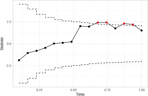
The three-level model estimates have an overall RMSE of 1.172. Figure 5 displays an example of a Shewhart chart monitoring the residuals of the first level $r_i^{(L_0)}.$ The chart signals four times near the end of the year. In total, the residuals charts signal 190 times (88 of which (46.32%) are exceptional courses), for 112 different students (36 of which (32.14%) are exceptional students).

Figure 5. Residual Shewhart control chart monitoring $r_i^{(L_0)}$ based on a three-level regression (signals in red).

As given by Eq. [3], we can also monitor the student level residuals using a Hotelling T² chart. Using the same data as in the previous, the T² chart signals at least once for 105 students (38 (36.19%) of which are exceptional students).

The charts signal exceptional cases throughout the year. However, we cannot retrospectively determine if at the time of a signal there was some unknown factor that influenced the performance of student j for course i. We are thus unable to distinguish false from true signals. It does, however, out-of-the-box, identify students whom we know have interesting performance during the monitoring phase.

The statistical monitoring approach identifies incidental anomalies in the weighted averages. However, the school’s main focus is to identify students who need either support or more challenging coursework. This monitoring approach is insufficient for that goal. Therefore, in the next section, we use the hierarchical model to monitor student expected end-of-year results to identify under- or overperforming students.

4.2. Predictive monitoring

The high school in this case study aims to predict the end-of-year grades of its students. This enables the school to receive early warnings on exceptional students. In this section, we will thus consider predictive monitoring of student performance.

4.2.1. Multilevel predictive monitoring

As demonstrated in Section 3.3, the predictions of the three-level model are relatively accurate. Furthermore, the three-level model can be used for new students/classes and when there are a small number of courses per student or students per class. In this section, we will thus use the three-level model for predictive monitoring.

We want to monitor $P{(E)}_t,$ defined as the probability of some event E at time t. $P{(E)}_t$ summarizes the outcome of the model into a single predictive probability at time t, with $t\in \{t_I,T\}$ where t_I indicates the start of the year and T the end of the year. The chart signals when $P{(E)}_t$ exceeds threshold C, which is defined as the maximum allowed probability of event E occurring ($0<C<1$). Event E concerns the values of y_i, which is context dependent and can take many forms (y_i = e, $y_i\ge e,y_i\le e,e_1\le y_i\le e_2,{\sum }_{i=a}^b{y}_i\ge e$ etc., where $e,e_1$ and e₂ are arbitrary constants and a and b are integers between 1 and n₀). Following the MCMC estimation of the posterior densities of the parameters $\mathit{\theta }=\{{\mathit{\beta }}^{({\mathit{L}}_{\mathbf{0}})},{\sigma }^2,{\mathit{\beta }}^{({\mathit{L}}_{\mathbf{1}})},{\Sigma }^{({\mathit{L}}_{\mathbf{1}})},{\mathit{\beta }}^{({\mathit{L}}_{\mathbf{2}})},{\Sigma }^{({\mathit{L}}_{\mathbf{2}})}\}$ as described in the supplementary material, we can use the posterior densities to calculate $P{(E)}_t.$

The steps for predictive monitoring are

1. Define event E and threshold C

2. Specify the multilevel model for y_i

3. Estimate the parameters to obtain ${\widehat{\mathit{\theta }}}_{\mathit{I}}$ using the phase I data at time t_I using MCMC, described in the appendix

4. Calculate $P{(E)}_t$ using the newly available observations at time $t>t_I$

5. Signal if $P{(E)}_t>C$

6. Re-estimate the parameters to obtain ${\widehat{\theta }}_{\mathit{t}}$ using all available data at time t and go back to step 4 for a new timepoint $t_{II}>t.$

Assume that we have a large in-control phase I data set $\{{\mathit{X}}_{\mathit{I}}^{({\mathit{L}}_{\mathbf{0}})},{\mathit{X}}_{\mathit{I}}^{({\mathit{L}}_{\mathbf{1}})},{\mathit{X}}_{\mathit{I}}^{({\mathit{L}}_{\mathbf{2}})},{\mathit{y}}_{\mathit{I}}\}$ at time t = t_I. At time $t<t_I$ we obtain the estimates for the parameters $\{{\widehat{\mathit{\beta }}}_{}^{({\mathit{L}}_{\mathbf{0}})},{\widehat{\sigma }}^2,{\widehat{\mathit{\beta }}}_{}^{({\mathit{L}}_{\mathbf{1}})},{\widehat{\Sigma }}^{({\mathit{L}}_{\mathbf{1}})},{\widehat{\mathit{\beta }}}^{({\mathit{L}}_{\mathbf{2}})},{\widehat{\Sigma }}^{({\mathit{L}}_{\mathbf{2}})}\}$ based on observations in phase I. As described in the appendix for the three-level model, using the estimates of the parameters, at any time $t>t_I$ we have a predicted distribution for the outcome variable ${\widehat{y}}_{i,t}$ $$\begin{array}{c}{\widehat{y}}_{i,t}\sim N(({\mathit{X}}_{i,t}^{(L_0)}\otimes {\mathit{X}}_{j[i,t]}^{(L_1)\prime }){\widehat{\mathit{\beta }}}^{(L_2)}{\mathit{X}}_{h\left[j\right[i,t\left]\right]}^{(L_2)\prime },\\ ({\mathit{X}}_{i,t}^{(L_0)}\otimes {\mathit{X}}_{j[i,t]}^{(L_1)}){\widehat{\mathbf{\Sigma }}}^{(L_2)}({\mathit{X}}_{i,t}^{(L_0)}\otimes {\mathit{X}}_{j[i,t]}^{(L_1)\prime })+{\mathit{X}}_{i,t}^{(L_0)}{\widehat{\mathbf{\Sigma }}}^{(L_1)}{\mathit{X}}_{i,t}^{(L_0)\prime }+{\widehat{\sigma }}^2),\end{array}$$ where ⊗ is the Kronecker product. We can use this result to estimate the probability of the outcome $P{(E)}_t.$ The event E can take several forms. Suppose we consider $y_i\le e,$ i.e. we study that the grade y_i is less than e. The monitoring scheme we propose uses the posterior distribution of ${\widehat{y}}_{i,t}$ to calculate the probability $P{(E)}_t.$ The chart signals when $P{(E)}_t>C,$ with C the threshold that determines the maximum allowed probability of event E.

Monitoring $P{(E)}_t$ requires periodic re-estimation of the parameters to incorporate newly available information at time t. Around the time event E occurs, the probability $P{(E)}_t$ converges to 1 if $t\to T.$ The major advantage of monitoring $P{(E)}_t$ instead of $y_{i,t}$ is that, depending on the predictive capability of the multilevel model, the monitoring scheme provides early warning and the opportunity to intervene before event E occurs. If intervention occurs, it is important to include this in the predictors $\{{\mathit{X}}^{({\mathit{L}}_{\mathbf{0}})},{\mathit{X}}^{({\mathit{L}}_{\mathbf{1}})},{\mathit{X}}^{({\mathit{L}}_{\mathbf{2}})}\}$ by including an additional variable, to extract the effect of the intervention on outcome E. Furthermore, there is no need for n₀ control charts. All that is required is a single control chart plotting values of $P{(E)}_t$ and signaling for observations or groups for which $P{(E)}_t$ exceeds C.

4.2.2. Example

Following the steps outlined before, we define two events: E^f as a student failing the year and E^e as a student excelling that year. E^f occurs if a student has four or more failpoints, as defined in the previous section (the number of points below 6 for all courses a student follows in a year). E^e occurs if a student has four or more excelpoints (the number of points above 8 for all courses a student follows in a year).

The end-of-year rounded grade of student j for course i is defined as y_ij. At time t, the probability of a student failing the year can thus be summarized by $P{(E_j^f)}_t=P{({\sum }_{i=1}^{n_j}\max (0,(6-y_{ij}))\ge 4)}_t,$ where n_j is the number of courses for student j. The probability of a student excelling in the year can then be summarized by $P{(E_j^e)}_t=P{({\sum }_{i=1}^{n_j}\max (0,(y_{ij}-8))\ge 4)}_t$ at time t.

Using the same data set as in the previous section, Figure 6 shows a control chart of $1-P{(E_j^f)}_t$ for J = 268 students at 15 points in time. As an example, the threshold C = 0.05 is depicted as a dashed line. Note that $1-P{(E_j^f)}_t$ equals the probability of passing the year. The J_p = 238 students who passed are depicted in blue and the probabilities of the J_f = 30 students who failed in red. Although there are some exceptions, overall the model consistently estimates the passing probabilities for the students who fail the year much lower than the students who pass the year. This can also be seen in the probabilities of failure in Table 5. This table reports the values of $\frac{1}{J_p}\sum _{j\in J_p}P{(E_j^f)}_t$ (the average estimated probability of failure for students that pass the year) in the top row and $\frac{1}{J_f}\sum _{j\in J_f}P{(E_j^f)}_t$ (the average estimated probability of failure for students that fail the year) in the bottom row. The model consistently assigns a higher average probability of failure to students that end up failing the year.

Figure 6. A control chart monitoring the estimated probabilities of passing $1-P{(E^f)}_t$ for 268 students in 2014/2015, with dashed threshold C = 0.05 in black. The dashed blue lines represent students that passed, the red solid lines students that failed.

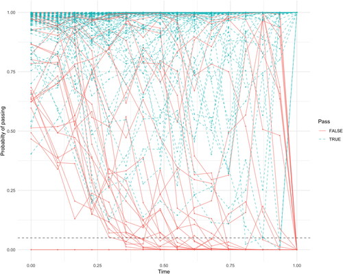
Table 5. Average estimated probabilities of failing $P{(E^f)}_t$ for 268 students in 2014/2015, split by observed outcome.

	Time
Failed	0	0.1	0.3	0.5	0.7	0.9	1
No	0.02	0.02	0.04	0.03	0.03	0.01	0.00
Yes	0.27	0.28	0.52	0.61	0.75	0.79	1.00

Figure 7 plots $P{(E_j^e)}_t$ for the same J = 268 students. The J_n = 222 students who did not excel are depicted in red and the probabilities of the J_e = 46 students who excelled are depicted in blue. As an example, threshold C = 0.95 is depicted as a dashed line. The model has impressive performance, shown also by the differences in average probabilities over time between students who excel, $\frac{1}{J_e}\sum _{j\in J_e}P{(E_j^e)}_t,$ and those that do not, $\frac{1}{J_n}\sum _{j\in J_n}P{(E_j^e)}_t,$ as depicted in Table 6.

Figure 7. A control chart monitoring the estimated probabilities of excelling $P{(E^e)}_t$ for 268 students in 2014/2015, with dashed threshold C = 0.95 in black. The solid blue lines represent students that excelled, the red dashed lines students that did not excel.

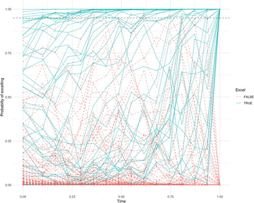
Table 6. Average estimated probabilities of excelling $P{(E^e)}_t$ for 268 students in 2014/2015, split by observed outcome.

	Time
Excelled	0	0.1	0.3	0.5	0.7	0.9	1
No	0.05	0.04	0.04	0.06	0.04	0.03	0.00
Yes	0.50	0.49	0.50	0.61	0.67	0.81	1.00

Depending on the threshold C that determines if the monitoring scheme signals, the model correctly identifies several students who will fail/excel as well as some false positives. Tables 7 and 8 report the precision and recall values monitoring E^f and E^e, respectively, where the precision is defined as $${\text{Precision}}_t(C)=\frac{t{p}_t(C)}{t{p}_t(C)+f{p}_t(C)}$$ with $t{p}_t(C)$ equal to the number of true positives at time t for threshold C and $f{p}_t(C)$ the number of false positives at time t for threshold C. The recall is given by $${\text{Recall}}_t(C)=\frac{t{p}_t(C)}{t{p}_t(C)+f{n}_t(C)}$$ where $f{n}_t(C)$ equals the number of false negatives at time t for threshold C (Powers 2011).

Table 7. Precision${}_t(C)$ (Recall${}_t(C)$) results when monitoring $P{(E^f)}_t$ with various values of C and t using the three-level model predictions of end-of-year grades for 268 students in 2014/2015.

C
		0.05	0.1	0.25	0.5	0.75	0.999
Time	0	1 (0.07)	1 (0.07)	1 (0.07)	0.67 (0.13)	0.74 (0.47)	0.25 (0.93)
	0.1	1 (0.07)	1 (0.07)	1 (0.07)	1 (0.27)	0.71 (0.40)	0.25 (0.93)
	0.3	1 (0.10)	1 (0.20)	0.85 (0.37)	0.76 (0.53)	0.67 (0.67)	0.27 (1)
	0.5	1 (0.33)	1 (0.43)	0.94 (0.53)	0.79 (0.63)	0.67 (0.67)	0.34 (0.97)
	0.7	1 (0.57)	1 (0.63)	0.88 (0.73)	0.77 (0.70)	0.70 (0.77)	0.40 (0.97)
	0.9	0.90 (0.63)	0.86 (0.63)	0.88 (0.70)	0.81 (0.70)	0.81 (0.73)	0.59 (0.90)
	1	1 (1)	1 (1)	1 (1)	1 (1)	1 (1)	1 (1)

Table 8. Precision${}_t(C)$ (Recall${}_t(C)$) results when monitoring $P{(E^e)}_t$ with various values of C and t using the three-level model predictions of end-of-year grades for 268 students in 2014/2015.

C
		0.99	0.95	0.75	0.5	0.25	0.01
Time	0	1 (0.02)	1 (0.09)	0.93 (0.3)	0.85 (0.5)	0.69 (0.72)	0.38 (0.89)
	0.1	1 (0.04)	1 (0.2)	0.94 (0.35)	0.72 (0.46)	0.71 (0.65)	0.45 (0.87)
	0.3	1 (0.09)	1 (0.28)	0.89 (0.37)	0.83 (0.54)	0.68 (0.54)	0.45 (0.85)
	0.5	1 (0.37)	1 (0.41)	0.92 (0.52)	0.77 (0.59)	0.65 (0.67)	0.47 (0.96)
	0.7	1 (0.43)	1 (0.48)	0.89 (0.54)	0.88 (0.61)	0.72 (0.78)	0.57 (0.93)
	0.9	1 (0.57)	1 (0.63)	0.94 (0.74)	0.88 (0.83)	0.8 (0.87)	0.64 (1)
	1	1 (1)	1 (1)	1 (1)	1 (1)	1 (1)	1 (1)

Table 7 shows the procedure correctly identifies students who will fail the year early on. The performance is impressive, where, depending on the chosen level of C, multiple early warnings are generated aiding in the student support system. For example, setting C at 0.75, the procedure identifies almost half (14 out of 30) of the students who will fail before the start of the year with only 26% (5) false positives.

Table 8 shows the precision and recall values when predicting excelling students. Depending on the school’s preferences, high precision or recall can be achieved early on in the year. For example, setting C at 0.50, the procedure identifies half (23 out of 46) of the students who will excel before the start of the year with only 15% (4) false positives.

The multilevel monitoring procedure has shown its value in a high school setting, as it adequately provides expected end-of-year grades for all students and subjects. This can aid in classifying at-risk students who need support, as well as the areas in which they need help. On the other side of the spectrum, the model successfully identifies excelling students who can benefit from more challenging schoolwork. The model further provides easily interpretable results, as well as good explainability for the parameters.

5. Conclusions

This case study has considered three research questions concerning high school students’ performance. We worked together with a Dutch high school in attempting to answer the following questions (1) What determines student performance? (2) How can statistical process monitoring be used in monitoring student progress? (3) What method can be used for predictive monitoring of student results? This resulted in the use of a three-level model in a predictive monitoring scheme that can be applied when monitoring hierarchical data. We discuss our results in the following.

5.1. What determines student performance?

The detailed data set made available by a Dutch high school has shown interesting determinants of student performance. These are generally in line with the educational literature and are useful when monitoring student progress.

Female students were found to obtain higher final grades. In line with the literature, students with disabilities perform slightly worse. Children with highly educated parents outperform their peers with less-educated parents in this case study.

The nationality and language barrier variables represent an interesting case study of the discussed theory on immigrant and language barriers in academia. Consistent with work by Geay, McNally, and Telhaj (2013) and the “language broker” effect of Buriel et al. (1998), students born abroad achieve similar results to their locally born peers. A serious language barrier does seem to produce slightly lower grades. This, in turn, is consistent with findings by Kennedy and Park (1994) and Collier (1995).

Students show a decrease in performance through their high school career, with around half a point difference in grades between the first and fourth years of high school. Absences seem to have a strong negative correlation with grades, which justifies the penalization of these types of absences. On a policy level, the relationship between the primary school test scores (CITO) and student grades should be considered toward current discussion around the determinants of the high school level.

The main goal of the school was to monitor student performance as the process output throughout the year. Therefore, statistical and predictive monitoring techniques were considered.

5.2. Statistical process monitoring

Classical statistical process monitoring techniques are often insufficient when applied to complex processes, for which increasingly large data sets are available. When a hierarchical structure is present in the data set, multilevel modeling improves the reliability of process monitoring. Using multilevel models improve estimation accuracy and explainability over regular linear regression models. Furthermore, the method is essential for predictive modeling of new students/classes or students/classes with small sample sizes.

Univariate statistical process monitoring techniques proved insufficient in this case study and one-level linear regression models did not provide satisfactory results. We have discussed a three-level model together with the monitoring options. Residual control charting at the three levels was proposed as the multilevel statistical monitoring method for online monitoring of process output. The proposed multilevel monitoring framework did provide promising results.

5.3. Predictive monitoring

A predictive monitoring method has been developed to enable an early warning monitoring system. This method monitors the probability of an event, rather than a process output. The three-level model was used to continuously predict end-of-year individual grades. Using a Bayesian hierarchical model, probability distributions for the student outcomes are obtained. These can be used to monitor unwanted results in the form of under- and overperforming students using a single predictive control chart setup. This predictive monitoring approach was shown to be very useful in practice, as the school obtains valuable early warnings on both under- and overperforming students.

The proposed multilevel process monitoring framework can be useful across many applications, including industrial processes (batch production, multiple factories), market monitoring, HR analytics, sports and more. Implementation of multilevel models can be challenging, however, especially in a Bayesian setting. Sampling procedures can be used to simplify the analysis. We have provided a full analysis of the three-level model and its estimation in the supplementary material, where we used Gibbs sampling to estimate the parameters. Using these parameters, predictions were made for the monitoring period, after which the parameters can be updated to improve the predictive power of the model. Predictive monitoring results in early warning systems, that can greatly aid in early detection and prevention of special cause variation.

We argue the importance of predictive monitoring in general. As more and more data are available, the use of more complex models can extract more information toward valuable predictions. Summarizing complex processes into simple and interpretable results is essential. Multilevel modeling is one method that achieves this, which is applicable in cases where a clear hierarchy is present. There are of course many more statistical and machine learning methods that can be applied. We encourage research that investigates the use of these methods in a predictive monitoring setting.

Concluding this paper, early warning indicator systems have the potential to improve the educational system at a low cost. These systems can add a layer of sophistication to school and teacher performance evaluation and work toward fulfilling individual student needs.

Acknowledgments

We want to thank the Dutch high school for participating in this project and sharing the valuable data. We are grateful to Dr. Reza Mohammadi and Dr. Maurice Bun (University of Amsterdam) and Dr. Inez Zwetsloot (City University of Hong Kong) for their helpful comments. We also thank the referees and the case studies department editor for their valuable suggestions to improve the paper.

Disclosure statement

No potential conflict of interest was reported by the authors.

Additional information

Notes on contributors

Leo C. E. Huberts

Leo C. E. Huberts is a PhD student and lecturer at the Department of Operations Management and consultant at the Institute for Business and Industrial Statistics of the University of Amsterdam, the Netherlands. His current research topic is statistical and predictive process monitoring.

Marit Schoonhoven

Marit Schoonhoven is an associate professor at the Department of Operations Management and senior consultant at the Institute for Business and Industrial Statistics of the University of Amsterdam, the Netherlands. Her current research interests include control charting techniques and operations management methods.

Ronald J. M. M. Does

Ronald J. M. M. Does is professor of Industrial Statistics at the University of Amsterdam and Head of the Department of Operations Management at the Amsterdam Business School. He is a Fellow of the ASQ and ASA, an elected member of the ISI, and an Academician of the International Academy for Quality. His current research activities include the design of control charts for nonstandard situations, healthcare engineering, and operations management methods.

Appendix

A.1 Predictive distribution

If we represent the three-level model in the following way (A1) $$\begin{array}{c}{y}_i={\mathit{X}}_{\mathit{i}}^{({\mathit{L}}_{\mathbf{0}})}{\mathit{\beta }}_{\mathit{j}\left[\mathit{i}\right]}^{({\mathit{L}}_{\mathbf{0}})}+{\epsilon }_i^{(L_0)},{\epsilon }^{(L_0)}\sim N(0,{\sigma }_y^2)\\ {\mathit{\beta }}_{\mathit{j}}^{({\mathit{L}}_{\mathbf{0}})}={\mathit{\beta }}_{\mathit{h}\left[\mathit{j}\right]}^{({\mathit{L}}_{\mathbf{1}})}{\mathit{X}}_{\mathit{j}}^{({\mathit{L}}_{\mathbf{1}})\prime }+{\mathit{\epsilon }}_{\mathit{j}}^{({\mathit{L}}_{\mathbf{1}})},{\mathit{\epsilon }}^{({\mathit{L}}_{\mathbf{1}})}\sim N(0,{\mathbf{\Sigma }}^{({\mathit{L}}_{\mathbf{1}})})\\ vec({\mathit{\beta }}_{\mathit{h}}^{({\mathit{L}}_{\mathbf{1}})})={\mathit{\beta }}^{({\mathit{L}}_{\mathbf{2}})}{\mathit{X}}_{\mathit{h}}^{({\mathit{L}}_{\mathbf{2}})\prime }+{\mathit{\epsilon }}_{\mathit{h}}^{({\mathit{L}}_{\mathbf{2}})},{\mathit{\epsilon }}^{({\mathit{L}}_{\mathbf{2}})}\sim N(0,{\mathbf{\Sigma }}^{({\mathit{L}}_{\mathbf{2}})})\end{array}$$(A1) we can summarize the model into $$y_i={\mathit{X}}_i^{(L_0)}ve{c}^{-1}({\mathit{\beta }}^{(L_2)}{\mathit{X}}_{h\left[j\right[i\left]\right]}^{(L_2)\prime }){\mathit{X}}_{j\left[i\right]}^{(L_1)\prime }+{\mathit{X}}_i^{(L_0)}ve{c}^{-1}({\mathit{\epsilon }}_h^{(L_2)}){\mathit{X}}_{j\left[i\right]}^{(L_1)\prime }+{\mathit{X}}_i^{(L_0)}{\mathit{\epsilon }}_{j\left[i\right]}^{(L_1)}+{\epsilon }_i^{(L_0)}.$$

We obtain parameter estimates $\{{\widehat{\mathit{\beta }}}_{}^{({\mathit{L}}_{\mathbf{0}})},{\widehat{\sigma }}^2,{\widehat{\mathit{\beta }}}_{}^{({\mathit{L}}_{\mathbf{1}})},{\widehat{\Sigma }}^{({\mathit{L}}_{\mathbf{1}})},{\widehat{\mathit{\beta }}}^{({\mathit{L}}_{\mathbf{2}})},{\widehat{\Sigma }}^{({\mathit{L}}_{\mathbf{2}})}\}$ using the observations during phase I time period $t<t_I.$ At any time $t>t_I$ we have a predicted distribution for the outcome variable ${\widehat{y}}_{i,t}.$ Considering the distributions of the error terms ${\widehat{y}}_{i,t}$ has a normal distribution $$\begin{array}{c}{\widehat{y}}_{i,t}\sim N(({\mathit{X}}_{j[i,t]}^{(L_1)}\otimes {\mathit{X}}_{i,t}^{(L_0)}){\widehat{\mathit{\beta }}}^{(L_2)}{\mathit{X}}_{h\left[j\right[i,t\left]\right]}^{(L_2)\prime },\\ ({\mathit{X}}_{j[i,t]}^{(L_1)}\otimes {\mathit{X}}_{i,t}^{(L_0)}){\widehat{\mathbf{\Sigma }}}^{(L_2)}({\mathit{X}}_{j[i,t]}^{(L_1)}\otimes {\mathit{X}}_{i,t}^{(L_0)})\prime +{\mathit{X}}_{i,t}^{(L_0)}{\widehat{\mathbf{\Sigma }}}^{(L_1)}{\mathit{X}}_{i,t}^{(L_0)\prime }+{\widehat{\sigma }}^2),\end{array}$$ where ⊗ is the Kronecker product and we use the relationship $\mathit{vec}(\mathit{ABC})=(C\prime \otimes A)\mathit{vec}(B).$

A.2 Prior distributions

The full parameter space $\mathit{\theta }=\{{\mathit{\beta }}^{({\mathit{L}}_{\mathbf{0}})},{\sigma }^2,{\mathit{\beta }}^{({\mathit{L}}_{\mathbf{1}})},{\mathbf{\Sigma }}^{({\mathit{L}}_{\mathbf{1}})},{\mathit{\beta }}^{({\mathit{L}}_{\mathbf{2}})},{\mathbf{\Sigma }}^{({\mathit{L}}_{\mathbf{2}})}\},$ where ${\mathit{\beta }}^{({\mathit{L}}_{\mathbf{0}})}$ and ${\mathit{\beta }}^{({\mathit{L}}_{\mathbf{1}})}$ are constructed by stacking the parameter matrices ${\mathit{\beta }}_{\mathit{j}}^{({\mathit{L}}_{\mathbf{0}})}$ and ${\mathit{\beta }}_{\mathit{h}}^{({\mathit{L}}_{\mathbf{1}})}$ for all groups j and h respectively, are estimated using the Gibbs sampler (Casella and George 1992). The Gibbs sampler approximates the posterior distribution by sampling from the full conditional distributions of the parameters. We use the rJAGS package in R to link to JAGS (Plummer 2018).

The estimation requires prior distributions for the unknown parameter space. Parameters ${\mathit{\beta }}^{({\mathit{L}}_{\mathbf{0}})}$ and ${\mathit{\beta }}^{({\mathit{L}}_{\mathbf{1}})}$ have priors given explicitly by the model. Proper diffuse priors are chosen for parameters $\{{\sigma }^2,{\mathbf{\Sigma }}^{({\mathit{L}}_{\mathbf{1}})},{\mathit{\beta }}^{({\mathit{L}}_{\mathbf{2}})},{\mathbf{\Sigma }}^{({\mathit{L}}_{\mathbf{2}})}\}.$

The vector $\mathit{vec}({\mathit{\beta }}^{(L_2)})$ has a multivariate normal prior $N(\mathit{a},\mathit{B}),$ with diagonal covariance matrix $\mathit{B}$ and larger values of $\mathit{B}$ reflecting greater uncertainty. Thus proper but diffuse priors were determined, with $\mathit{a}=0$ and $\mathit{B}=1000\mathit{I},$ where $\mathit{I}$ is the identity matrix.

The covariance matrix ${\mathbf{\Sigma }}^{(L_1)}$ associated with level 1 student unobserved differences and the covariance matrix ${\mathbf{\Sigma }}^{(L_2)}$ for unobserved group level 2 differences are both defined as positive definite matrices with Inverse Wishart priors $W^{-1}(\mathit{C},(p_0+1)+1)$ for ${\mathbf{\Sigma }}^{(L_1)}$ and prior $W^{-1}(\mathit{D},(p_0+1)(p_1+1)+1)$ for ${\Sigma }^{(L_2)}.$ $\mathit{C}$ and $\mathit{D}$ are diagonal matrices, where smaller values correspond to more diffuse priors. Values for these inverse Wishart distributions are set at $\mathit{C}=\mathit{D}=\mathit{diag}(0.001).$

For the variance parameter ${\sigma }^2$ of the error term in the model the inverse Gamma distribution, IG(a, b), was chosen. We use an uniformative prior, with parameters $a=0.001;b=1;$ ${\sigma }^2\sim IG(0.001,1).$

References

- Aaronson, D. 1998. Using sibling data to estimate the impact of neighborhoods on children’s educational outcomes. The Journal of Human Resources 33 (4):915–46. doi: https://doi.org/10.2307/146403.
- Aitkin, M., and N. Longford. 1986. Statistical modelling issues in school effectiveness studies. Journal of the Royal Statistical Society: Series A (General) 149 (1):1–26. doi: https://doi.org/10.2307/2981882.
- Baghdadi, A., L. A. Cavuoto, A. Jones-Farmer, S. E. Rigdon, E. T. Esfahani, and F. M. Megahed. 2019. Monitoring worker fatigue using wearable devices: A case study to detect changes in gait parameters. Journal of Quality Technology :1–25. doi: https://doi.org/10.1080/00224065.2019.1640097.
- Banerjee, S., B. P. Carlin, and A. E. Gelfand. 2014. Hierarchical modeling and analysis for spatial data. London: Chapman and Hall/CRC.
- Battin-Pearson, S., M. D. Newcomb, R. D. Abbott, K. G. Hill, R. F. Catalano, and J. D. Hawkins. 2000. Predictors of early high school dropout: A test of five theories. Journal of Educational Psychology 92 (3):568–82. doi: https://doi.org/10.1037/0022-0663.92.3.568.
- Becker, J., L. S. Hall, B. Levinger, A. Sims, and A. Whittington. 2014. Student success and college readiness: Translating predictive analytics into action. Strategic Data Project, SDP Fellowship Capstone Report. http://sdp.cepr.harvard.edu/files/cepr-sdp/files/sdp-fellowship-capstone-student-success-college-readiness.pdf
- Berendsen, H. J. 2007. Simulating the physical world: Hierarchical modeling from quantum mechanics to fluid dynamics. Cambridge: Cambridge University Press.
- Bock, R. D. 1989. Multilevel analysis of educational data. San Diego, CA: Academic Press.
- Browne, W. J., and D. Draper. 2006. A comparison of Bayesian and likelihood-based methods for fitting multilevel models. Bayesian Analysis 1 (3):473–514. doi: https://doi.org/10.1214/06-BA117.
- Buriel, R., W. Perez, T. L. de Ment, D. V. Chavez, and V. R. Moran. 1998. The relationship of language brokering to academic performance, biculturalism, and self-efficacy among Latino adolescents. Hispanic Journal of Behavioral Sciences 20 (3):283–97. doi: https://doi.org/10.1177/07399863980203001.
- Casella, G., and E. I. George. 1992. Explaining the Gibbs sampler. The American Statistician 46 (3):167–74. doi: https://doi.org/10.2307/2685208.
- Collier, V. P. 1995. Acquiring a second language for school. Directions in Language and Education 1 (4):3–13.
- Deary, I. J., S. Strand, P. Smith, and C. Fernandes. 2007. Intelligence and educational achievement. Intelligence 35 (1):13–21. doi: https://doi.org/10.1016/j.intell.2006.02.001.
- Geay, C., S. McNally, and S. Telhaj. 2013. Non-native speakers of English in the classroom: What are the effects on pupil performance? The Economic Journal 123 (570):F281–307. doi: https://doi.org/10.1111/ecoj.12054.
- Geiser, S., and M. V. Santelices. 2007. Validity of high-school grades in predicting student success beyond the freshman year: High-school record vs. standardized tests as indicators of four-year college outcomes. UC Berkeley: Center for Studies in Higher Education 6 (7):1–35.
- Gelman, A. 2006. Multilevel (hierarchical) modeling: What it can and cannot do. Technometrics 48 (3):432–5. doi: https://doi.org/10.1198/004017005000000661.
- Henderson, C. R., O. Kempthorne, S. R. Searle, and C. M. von Krosigk. 1959. The estimation of environmental and genetic trends from records subject to culling. Biometrics 15 (2):192–218. doi: https://doi.org/10.2307/2527669.
- Hox, J. J., M. Moerbeek, and R. Van de Schoot. 2017. Multilevel analysis: Techniques and applications. London: Routledge.
- Kang, L., and S. L. Albin. 2000. On-line monitoring when the process yields a linear profile. Journal of Quality Technology 32 (4):418–26. doi: https://doi.org/10.1080/00224065.2000.11980027.
- Kang, L., X. Kang, X. Deng, and R. Jin. 2018. A Bayesian hierarchical model for quantitative and qualitative responses. Journal of Quality Technology 50 (3):290–308. doi: https://doi.org/10.1080/00224065.2018.1489042.
- Karande, S., and M. Kulkarni. 2005. Poor school performance. Indian Journal of Pediatrics 72 (11):961–7. doi: https://doi.org/10.1007/BF02731673.
- Kennedy, E., and H.-S. Park. 1994. Home language as a predictor of academic achievement: A comparative study of Mexican- and Asian-American youth. Journal of Research & Development in Education 27 (3):188–94.
- Laidra, K., H. Pullmann, and J. Allik. 2007. Personality and intelligence as predictors of academic achievement: A cross-sectional study from elementary to secondary school. Personality and Individual Differences 42 (3):441–51. doi: https://doi.org/10.1016/j.paid.2006.08.001.
- Laurenceau, J.-P., L. F. Barrett, and M. J. Rovine. 2005. The interpersonal process model of intimacy in marriage: A daily-diary and multilevel modeling approach. Journal of Family Psychology 19 (2):314–23. doi: https://doi.org/10.1037/0893-3200.19.2.314.
- Mandel, B. J. 1969. The regression control chart. Journal of Quality Technology 1 (1):1–9. doi: https://doi.org/10.1080/00224065.1969.11980341.
- Montgomery, D. C. 2007. Introduction to statistical quality control. Hoboken, NJ: John Wiley & Sons.
- Nichols, J. D. 2003. Prediction indicators for students failing the state of Indiana high school graduation exam. Preventing School Failure: Alternative Education for Children and Youth 47 (3):112–20. doi: https://doi.org/10.1080/10459880309604439.
- Nichols, J. D., and J. White. 2001. Impact of peer networks on achievement of high school algebra students. The Journal of Educational Research 94 (5):267–73. doi: https://doi.org/10.1080/00220670109598762.
- Parker, J. D., M. J. Hogan, J. M. Eastabrook, A. Oke, and L. M. Wood. 2006. Emotional intelligence and student retention: Predicting the successful transition from high school to university. Personality and Individual Differences 41 (7):1329–36. doi: https://doi.org/10.1016/j.paid.2006.04.022.
- Plummer, M. 2018. rjags: Bayesian graphical models using MCMC. R package version 4-8. https://CRAN.R-project.org/package=rjags
- Powers, D. M. W. 2011. Evaluation: from precision, recall and F-measure to ROC, informedness, markedness and correlation. Journal of Machine Learning Technologies 2 (1):37–63.
- Qiu, P., C. Zou, and Z. Wang. 2010. Nonparametric profile monitoring by mixed effects modeling. Technometrics 52 (3):265–77. doi: https://doi.org/10.1198/TECH.2010.08188.
- Rahafar, A., M. Maghsudloo, S. Farhangnia, C. Vollmer, and C. Randler. 2016. The role of chronotype, gender, test anxiety, and conscientiousness in academic achievement of high school students. Chronobiology International 33 (1):1–9. doi: https://doi.org/10.3109/07420528.2015.1107084.
- Rohde, T. E., and L. A. Thompson. 2007. Predicting academic achievement with cognitive ability. Intelligence 35 (1):83–92. doi: https://doi.org/10.1016/j.intell.2006.05.004.
- Romero, C., and S. Ventura. 2019. Guest editorial: Special issue on early prediction and supporting of learning performance. IEEE Transactions on Learning Technologies 12 (2):145–7. doi: https://doi.org/10.1109/TLT.2019.2908106.
- Rothman, S. 2001. School absence and student background factors: A multilevel analysis. International Education Journal 2 (1):59–68.
- Rothstein, J. M. 2004. College performance predictions and the SAT. Journal of Econometrics 121 (1-2):297–317. doi: https://doi.org/10.1016/j.jeconom.2003.10.003.
- Sang, H., and A. E. Gelfand. 2009. Hierarchical modeling for extreme values observed over space and time. Environmental and Ecological Statistics 16 (3):407–26. doi: https://doi.org/10.1007/s10651-007-0078-0.
- Schirru, A., S. Pampuri, and G. De Nicolao. 2010. Multilevel statistical process control of asynchronous multi-stream processes in semiconductor manufacturing. In 2010 IEEE International Conference on Automation Science and Engineering, 57–62, Toronto, ON, Canada.
- Sellström, E., and S. Bremberg. 2006. Is there a “school effect” on pupil outcomes? A review of multilevel studies. Journal of Epidemiology & Community Health 60 (2):149–55.
- Stewart, E. B. 2008. School structural characteristics, student effort, peer associations, and parental involvement: The influence of school-and individual-level factors on academic achievement. Education and Urban Society 40 (2):179–204. doi: https://doi.org/10.1177/0013124507304167.
- Sui-Chu, E. H., and J. D. Willms. 1996. Effects of parental involvement on eighth-grade achievement. Sociology of Education 69 (2):126–41. doi: https://doi.org/10.2307/2112802.
- Vining, G. 2009. Technical advice: Phase I and phase II control charts. Quality Engineering 21 (4):478–9. doi: https://doi.org/10.1080/08982110903185736.
- Wang, Y. F., S. T. Tseng, B. H. Lindqvist, and K. L. Tsui. 2019. End of performance prediction of lithium-ion batteries. Journal of Quality Technology 51 (2):198–213. doi: https://doi.org/10.1080/00224065.2018.1541388.
- Weese, M., W. Martinez, F. M. Megahed, and L. A. Jones-Farmer. 2016. Statistical learning methods applied to process monitoring: An overview and perspective. Journal of Quality Technology 48 (1):4–24. doi: https://doi.org/10.1080/00224065.2016.11918148.
- Woodall, W. H., and D. C. Montgomery. 2014. Some current directions in the theory and application of statistical process monitoring. Journal of Quality Technology 46 (1):78–94. doi: https://doi.org/10.1080/00224065.2014.11917955.