A comprehensive toolbox for the gamma distribution: The gammadist package

Abstract

The gamma distribution is one of the most important parametric models in probability theory and statistics. Although a multitude of studies have theoretically investigated the properties of the gamma distribution in the literature, there is still a serious lack of tailored statistical tools to facilitate its practical applications. To fill the gap, this paper develops a comprehensive R package for the gamma distribution. In specific, the R package focuses on the following three important tasks: generate the gamma random variables, estimate the model parameters, and construct statistical limits, including confidence limits, prediction limits, and tolerance limits based on the gamma random variables. The proposed package encompasses the state-of-the-art methods of the gamma distribution in the literature and its usage is illustrated by a real application.

Keywords:

• confidence interval
• estimation
• prediction interval
• sampling
• tolerance interval

1. Introduction

The gamma distribution is an important distribution that has received considerable attention in the probability and statistics literature. For example, due to its relation with the exponential distribution, the gamma distribution is frequently the probability model for waiting times (Lee and Wang 2011; Lin and Lin 2015). In quality and reliability engineering, the gamma distribution is extensively used to fit the product lifetimes, as it could exhibit decreasing, constant, and increasing failure rates (Chen and Ye 2018; Wang and Wu 2018). Moreover, the gamma distribution has shown to be an appropriate model in many other application areas including environments (Baran and Nemoda 2016), wireless communications (Al-Ahmadi and Yanikomeroglu 2010), geoscience (Gao et al. 2017), disaster monitoring (Xiao et al. 2021), and image analysis (El-Zaart 2010).

The gamma distribution Gam$(k,\theta )$ has probability density function (pdf) $$f(x)=\frac{1}{\Gamma (k){\theta }^k}{x}^{k-1}{e}^{-x/\theta },x>0,$$ where k > 0 is the shape parameter and $\theta >0$ is the scale parameter. In some applied fields, the parametrization with shape k and rate β, which is the inverse of θ, is more common. The mean and variance of Gam$(k,\theta )$ are $k\theta$ and $,$ respectively. The gamma distribution includes the exponential distribution (k = 1) and the Chi-square distribution (θ = 2) as its special cases, and the normal distribution ($k\to \infty$) as its limiting case. In addition, the gamma distribution is also closely related to the beta distribution, the Dirichlet distribution, and the F-distribution.

In order to successfully implement the gamma distribution in practice, some fundamental statistical issues need to be addressed. The first issue is about generating the gamma distributed random variables. In the literature, this task is often performed by considering $k\ge 1$ and k < 1 separately. Let $X\sim \text{Gam}(k,\theta ).$ Simulating X when $k\ge 1$ is generally easy as transformations of X (e.g., $\text{log}\hspace{0.17em}X$ and $X^{1/3}$) can be well approximated by a normal distribution. Using the normal distribution as the envelope, the gamma variates can be readily obtained by the acceptance-rejection method with low rejection rate (Ahrens and Dieter 1982; Marsaglia and Tsang 2000). This idea is employed by the default rgamma function in R for the $k\ge 1$ case. On the other hand, the k < 1 case is not easy to deal with as an adequate approximation for X is lacking under small shape parameter and, hence, a proper envelope is difficult to construct. Some tailored envelope functions directly applied to the gamma density have been proposed in the literature, including Ahrens and Dieter (1974); Best (1983); and Kundu and Gupta (2007), with the first one being used by the rgamma function. However, these envelope functions generally do not provide an overall tight bound on the gamma density and the corresponding accept-reject algorithm could yield a high rejection rate. For example, it is well known that the rgamma function in R is relatively inaccurate and inefficient in sampling when the shape parameter k is small (Liu, Martin, and Syring 2017). In view of this fact, some more efficient sampling methods based on the limiting distribution of $\text{log}\hspace{0.17em}X$ as $k\to 0$ have been proposed during recent years (Liu, Martin, and Syring 2017; Xi, Tan, and Liu 2013). In the proposed R package, a gamma random variable generator that suffices for all ranges of k will be developed.

The second important issue is how to estimate the gamma parameters based on the gamma distributed data. It is well known that the maximum likelihood (ML) estimators of the gamma parameters do not have closed-form expressions, and they have to be numerically obtained by algorithms such as the quasi-Newton method. However, these algorithms could easily fail to converge when the shape parameter k is small (Ye and Chen 2017). On the other hand, although the moment estimators of the gamma parameters have the closed forms, they are not efficient under either small or large samples. Recently, Ye and Chen (2017) proposed the ML-like closed-form estimators for the gamma parameters deriving from the generalized gamma distribution. The proposed estimators are shown to perform almost identically to the ML estimators in both finite and large samples. In addition, the proposed estimators are consistent and asymptotically normally distributed. Louzada, Ramos, and Ramos (2019) further improved the performance of the estimators in finite samples by considering bias correction, and these estimators will be integrated in the gammadist package.

The third task accomplished by the package is to construct some important statistical limits (intervals) of the gamma distribution, including the confidence limits, prediction limits, and tolerance limits (see, e.g., Hayter and Kiatsupaibul 2014). The confidence limits construction is undoubtedly a classical topic in statistics, as it quantifies uncertainties during point estimation. On the other hand, the prediction and tolerance limits are critical in knowing the properties of the future observations, which play fundamental roles in quality control and environment monitoring applications where the gamma distribution is a popular model. In the literature, there have been a multitude of methods of constructing these statistical limits for the gamma distribution. For example, the large-sample approximation or the bootstrap are often used to construct the confidence limits (see, e.g., Bhaumik, Kapur, and Gibbons 2009), while the normal-based method (see, e.g., Krishnamoorthy, Mathew, and Mukherjee 2008) and some complex analytical approximations (see, e.g., Bhaumik and Gibbons 2006) have been proposed for the other two statistical limits. One drawback of these methods is that their performance is not uniformly satisfactory in practice. For instance, the large-sample approximation and bootstrap only work well in large samples, and the normal-based method does not perform satisfactorily when the shape parameters are small. Until recently, the new paradigm of the generalized pivotal quantity (GPQ) has been developed for construing the statistical limits of the gamma distribution, and its uniformly outstanding performance has been verified by many studies (Chen and Ye 2017a, 2018; Wang and Wu 2018). In the gammadist package, the GPQ method will be implemented.

The remainder of the article will be organized as follows. Section 2 introduces the underlying methodologies used in the package, including random variable generation, parameter estimation, and statistical limits construction. Section 3 presents the gammadist package, which consists of six functions. For each function, its arguments and outputs are explicitly stated and its demos are shown in R code. Section 4 illustrates the package by a groundwater monitoring application. At last, Section 5 concludes the article and discusses some potential directions of extending the package.

2. Technical details

This section introduces the underlying technical details used in the gammadist package. The methods of generating random variables, estimating parameters, and constructing statistical limits will be discussed in the following subsections.

2.1. Random variable generation

As argued, we focus on generating gamma random variables when $0<k<1,$ as the default rgamma function in R is efficient when $k\ge 1.$ We only need to consider the random variable $Y\sim \text{Gam}(k,1)$ as the scale parameter could be multiplied afterwards, that is, $X=\theta \mathit{Y}\sim \text{Gam}(k,\theta ).$ Liu, Martin, and Syring (2017) considered the transformation $Z=-k\hspace{0.17em}\text{log}\hspace{0.17em}(Y)$ and observed that $Z\to \hspace{0.17em}\text{Exp}\hspace{0.17em}(1)$ in distribution as $k\to 0,$ where $\text{Exp}\hspace{0.17em}(1)$ denotes the unit-rate exponential distribution. In specific, the density function h(z) of Z is $$h(z)=c{e}^{-z-e^{-z/k}},z\in (-\infty ,\infty ),$$ where $c=1/\Gamma (k+1)$ is the normalization constant. It is easy to see that h(z) is log-concave, and it is ideally suited to acceptance-rejection sampling with two exponential envelopes oriented in opposite directions from the mode m = 0. This is because any line tangent to $\text{log}\hspace{0.17em}h(z)$ lies above $\text{log}\hspace{0.17em}h(z),$ while the log exponential density is a straight line. Thus, the aim is to find the two exponential envelopes that minimize the rejection rate. Toward this end, Liu, Martin, and Syring (2017) obtained the optimal envelop function as follows: $$\eta (z)=\{\begin{array}{cccc}\hfill & c{e}^{-z},\hfill & \hfill & \text{if}z\ge 0,\hfill \\ \hfill & cw\lambda e^{\lambda z},\hfill & \hfill & \text{if}z<0,\hfill \end{array}$$ where $w\equiv w(k)=k/[e(1-k)]$ and $\lambda \equiv \lambda (k)=(1/k)-1.$ Thus, the two exponential distributions are Exp(1) and -Exp(λ), respectively. In addition, the ratio of sampling from Exp(1) and -Exp(λ) is $1/w.$ Therefore, we only need to sample from the following mixture of two exponential distributions: [1] $$\frac{1}{1+w}\text{Exp}\hspace{0.17em}(1)+\frac{w}{1+w}[-\hspace{0.17em}\text{Exp}\hspace{0.17em}(\lambda )],$$[1] which can be easily achieved by the uniform random variable generators such as the runif function in R. Once a z is sampled from Eq. [1], it is accepted only if $h(z)/\eta (z)>u,$ where u is a realization of $\text{Unif}(0,1),$ that is, the standard uniform distribution. The gamma random variable can then be obtained based on the transformation relation $Z=-k\hspace{0.17em}\text{log}\hspace{0.17em}(Y).$ To summarize, Algorithm 1 shows the pseudo-code for generating the gamma random variables for all the range of k > 0.

Algorithm 1: Generation of the gamma random variables.

Input: Shape parameter k and scale parameter θ

Output: Gamma random variable $X\sim \text{Gam}(k,\theta )$

1 do

2  if $k\ge 1$ then

3   $X\leftarrow \mathsf{rgamma}(\mathit{k},\theta )$ // rgamma is the default function in R that generates gamma random variable with shape parameter k and scale parameter θ

4  end

5  else

6   $w\leftarrow k/e/(1-k);$ $\lambda \leftarrow 1/k-1;$ $r\leftarrow 1/(1+w)$

7   $U_1\leftarrow \mathsf{runif}(0,1)$ // runif(0,1) generates the standard uniform random variable

8   if $U_1\le r$ then

9    $z\leftarrow \mathsf{rexp}(1)$ // rexp(λ) generates the exponential random variable with rate λ

10   end

11   else

12    $z\leftarrow -\mathsf{rexp}(\lambda )$

13   end

14   $U_2\leftarrow \mathsf{runif}(0,1)$

15   if $h(z)/\eta (z)>U_2$ then

16    $Z\leftarrow z$

17    $Y\leftarrow \hspace{0.17em}\text{exp}\hspace{0.17em}(-Z/k)$

18    $X\leftarrow \theta Y$

19   end

20  end

21 until X is generated

2.2. Parameter estimation

The closed-form estimators proposed in Ye and Chen (2017) and Louzada, Ramos, and Ramos (2019) are used for parameter estimation. The underlying idea is to use the generalized gamma distribution GGam$(k,\theta ,b),$ which has pdf $$g(x)=\frac{b}{\Gamma (k){\theta }^{bk}}{x}^{bk-1}{e}^{-{(x/\theta )}^b},x>0.$$

When b = 1, the generalized gamma distribution degenerates to the gamma distribution. Let $X\sim \text{GGam}(k,\theta ,b)$ and $X_1,\dots ,X_n$ be independent and identically distributed copies of X. Thus, the score equations are $$\begin{array}{c}-\psi (k)-b\hspace{0.17em}\text{log}\hspace{0.17em}\theta +\frac{b}{n}\sum _i\hspace{0.17em}\text{log}\hspace{0.17em}{X}_i=0,\\ -k+\frac{1}{n}\sum _i{(X_i/\theta )}^b=0,\\ \frac{1}{b}+\frac{k}{n}\sum _i\hspace{0.17em}\text{log}\hspace{0.17em}(X_i/\theta )-\frac{1}{n}\sum _i{(X_i/\theta )}^b\hspace{0.17em}\text{log}\hspace{0.17em}(X_i/\theta )=0.\end{array}$$

By setting b = 1 in the above equations and noting $\beta =1/\theta ,$ the closed-form estimators for k, θ, and β could then be obtained as [2] $$\begin{array}{c}\widehat{k}=\frac{n\sum _i{X}_i}{n\sum _{i}Xi\hspace{0.17em}\text{log}\hspace{0.17em}{X}_i-\sum _i\hspace{0.17em}\text{log}\hspace{0.17em}{X}_i\sum _i{X}_i},\\ \widehat{\theta }=\frac{n\sum _i{X}_i\hspace{0.17em}\text{log}\hspace{0.17em}{X}_i-\sum _i\hspace{0.17em}\text{log}\hspace{0.17em}{X}_i\sum _i{X}_i}{n^2},\\ \widehat{\beta }=\frac{n^2}{n\sum _i{X}_i\hspace{0.17em}\text{log}\hspace{0.17em}{X}_i-\sum _i\hspace{0.17em}\text{log}\hspace{0.17em}{X}_i\sum _i{X}_i}.\end{array}$$[2]

Ye and Chen (2017) numerically showed that these estimators perform almost identically to the ML estimators in finite samples and they are nearly efficient in large samples. To facilitate small-sample applications, the authors further proposed the bias-corrected estimators for the parameters. Because the estimator of k is based on an asymptotic argument and it still has systematic biases in finite samples, Louzada, Ramos, and Ramos (2019) further proposed an improved version. The idea is to subtract the second-order bias of the ML estimator, and a useful approximation was proposed by the authors; see Louzada, Ramos, and Ramos (2019) for more technical details.

In summary, the bias-corrected estimators for k, θ, and β are, respectively, given by [3] $$\begin{array}{l}\tilde{k}=\widehat{k}-\frac{1}{n}\left[3\widehat{k}-\frac{2\widehat{k}}{3(1+\widehat{k})}-\frac{4\widehat{k}}{5{(1+\widehat{k})}^2}\right],\\ \tilde{\theta }=\frac{n}{n-1}\widehat{\theta }=\frac{n\sum _i{X}_i\hspace{0.17em}\text{log}\hspace{0.17em}{X}_i-\sum _i\hspace{0.17em}\text{log}\hspace{0.17em}{X}_i\sum _i{X}_i}{n(n-1)},\\ \tilde{\beta }=\frac{n-1}{n+2}\widehat{\beta }=\frac{n^2(n-1)}{(n+2)(n\sum _i{X}_i\hspace{0.17em}\text{log}\hspace{0.17em}{X}_i-\sum _i\hspace{0.17em}\text{log}\hspace{0.17em}{X}_i\sum _i{X}_i)},\end{array}$$[3] where the closed-form expressions of $\widehat{k},\widehat{\theta }$ and $\widehat{\beta }$ are given in Eq. [2]. Algorithm 2 illustrates the overall estimation procedures.

Algorithm 2: Estimation of the parameters of a gamma distribution.

Input: n observations $x_1,\dots ,x_n.$

Output: Estimates of k, θ and β.

1 Compute the closed-form estimators $\widehat{k},\widehat{\theta }$ and $\widehat{\beta }$ by using Eq. [2]

2 Compute the bias-corrected closed-form estimators $\tilde{k},\tilde{\theta }$ and $\tilde{\beta }$ by using Eq. [3]

2.3. Construction of statistical limits

In this section, the GPQ method will be implemented for constructing the statistical limits of the gamma distribution. We first give a brief introduction of the GPQ method. As its name stands for, GPQ is a generalization of the classical pivotal quantity, and it is particularly useful in constructing statistical limits in the presence of nuisance parameters. Since its first introduction by Weerahandi (1993), the GQP method has received significant attention in the literature for its outstanding performance in interval estimation; successful applications can be found in Krishnamoorthy, Mallick, and Mathew (2011), Chen and Ye (2017b), and Wang et al. (2021a), to name a few. Suppose that we are interested in making inference of one unknown parameter $\theta \in \mathit{\theta },$ where $\mathit{\theta }$ is the vector of all the unknown parameters. Then, ${\mathcal{G}}_{\theta }(\mathbf{X},\mathbf{x},\mathit{\theta }),$ which is a function of the random sample $\mathbf{X}=(X_1,\dots ,X_n),$ the observed data $\mathbf{x}=(x_1,\dots ,x_n)$ and the unknown parameters $\mathit{\theta },$ are a GPQ for θ if it satisfies the following two conditions:

• C1. ${\mathcal{G}}_{\theta }(\mathbf{X},\mathbf{x},\mathit{\theta })$ has a probability distribution that is free of unknown parameters $\mathit{\theta }.$

• C2. The observed pivotal, defined as ${\mathcal{G}}_{\theta }(\mathbf{x},\mathbf{x},\mathit{\theta }),$ only depends on θ, that is, it does not depend on the nuisance parameters.

Based on the distribution of ${\mathcal{G}}_{\theta }(\mathbf{X},\mathbf{x},\mathit{\theta }),$ the confidence interval for θ can be constructed, which is known as the generalized confidence interval (GCI). Asymptotically, the GCI achieves the exact coverage under some mild conditions (Hannig, Iyer, and Patterson 2006). Moreover, numerous studies in the literature showed the excellent performance of the GCI under small and moderate sample sizes (see, e.g., Krishnamoorthy, Lee, and Zhang 2017; Wang et al. 2021b).

2.3.1. GPQs for the gamma parameters

GPQs for the parameters of the gamma distribution were first developed in Chen and Ye (2017a, 2017b), and later the GPQ for the shape parameter k was improved by Wang and Wu (2018). In the R package, the GPQs proposed by Wang and Wu (2018) are used as they yield better performance in terms of the coverage probabilities. In specific, let $T=\hspace{0.17em}\text{log}\hspace{0.17em}(\tilde{X}/\overline{X})$ where $\tilde{X}=\prod _i{X}_i^{1/n}$ and $\overline{X}=\sum _i{X}_i/n.$ Iliopoulos (2016) showed the distribution of T only depends on the shape parameter k. Let $F(T|k)$ be the cumulative distribution function (cdf) of T and then $F(T|k)\sim U_k,$ where U_k follows the standard uniform distribution. In other words, $T=Q(U_k|k),$ where $Q(p|k)$ represents the pth quantile of T and it depends on k only. On the other hand, the quantiles could be approximated by the Cornish-Fisher expansion, that is, $$\begin{array}{l}Q(p|k)=z_p+\frac{1}{6}{\tilde{c}}_3(z_p^2-1)+\frac{1}{24}{\tilde{c}}_4(z_p^3-3z_p)-\frac{1}{36}{({\tilde{c}}_3)}^2(2z_p^3-5z_p)\\ +\frac{1}{120}{\tilde{c}}_5(z_p^4-6z_p^2+3)-\frac{1}{24}{\tilde{c}}_3{\tilde{c}}_4(z_p^4-5z_p^2+2)+\frac{1}{324}{({\tilde{c}}_3)}^3(12z_p^4-53z_p^2+17),\end{array}$$ where c_i is the ith cumulant of T, ${\tilde{c}}_i=c_i/{(c_2)}^{i/2}$ and z_p is the pth quantile of a standard normal distribution. The expressions of c_i’s are derived in Wang and Wu (2018) and they are given by $$\begin{array}{c}{c}_1\equiv c_1(k)=\hspace{0.17em}\text{log}\hspace{0.17em}(n)+\psi (k)-\psi (nk),\\ c_i\equiv c_i(k)=\frac{1}{n^{i-1}}{\psi }_{i-1}(k)-{\psi }_{i-1}(nk),\hspace{1em}i=2,3,\dots ,\end{array}$$ where $\psi (k)=\Gamma \prime (k)/\Gamma (k)$ is the digamma function and ${\psi }_i(·)$ is the ith derivative of $\psi (·).$ With all these treatments, the GPQ ${\mathcal{G}}_k$ for k can be readily obtained by solving [4] $$\text{log}\hspace{0.17em}(\tilde{x}/\overline{x})=c_1({\mathcal{G}}_k)+{[c_2({\mathcal{G}}_k)]}^{1/2}Q(U_k|{\mathcal{G}}_k),$$[4] where $\tilde{x}$ and $\overline{x}$ are the observed geometric and arithmetic means, respectively. As seen, the distribution of ${\mathcal{G}}_k$ only depends on the standard uniform distribution U_k, so the first condition (C1) is satisfied. In addition, the observed pivotal, where U_k is replaced by its observed value, is equal to k, so the second condition (C2) also holds. Therefore, ${\mathcal{G}}_k$ is a valid GPQ for k. Because T is stochastically strictly increasing in k (Iliopoulos 2016), the above equation can be easily solved by bisection search given a realization of U_k. As for the scale parameter θ, observe that $2n\overline{X}/\theta \sim {\chi }^2(2nk),$ a ${\chi }^2$ distribution with 2nk degrees of freedom. Conditional on ${\mathcal{G}}_k,$ the GPQ for θ can be constructed as $${\mathcal{G}}_{\theta }=2n\overline{x}/U_{\theta },$$ where $U_{\theta }\sim {\chi }^2(2n{\mathcal{G}}_k).$ It is easy to check that ${\mathcal{G}}_{\theta }$ is independent of k and θ and its observed value is equal to θ. Therefore, ${\mathcal{G}}_{\theta }$ is a valid GPQ for θ. Consequently, the GPQ for the rate parameter β is ${\mathcal{G}}_{\beta }=1/{\mathcal{G}}_{\theta }.$

The exact distributions of the GPQs are difficult to derive. Nevertheless, their realizations can be readily generated by using the Monte Carlo simulation, and the procedures are summarized in Algorithm 3.

Algorithm 3: Generation of the realizations of the GPQs of the gamma parameters.

Input: n observations $x_1,\dots ,x_n$ and the number of realizations B.

Output: B realizations of the GPQs of k, θ, and β.

1 $\tilde{x}\leftarrow \prod _i{x}_i^{1/n};$ $\overline{x}\leftarrow \sum _i{x}_i/n$

2 for i in 1:B do

3  $U_k\leftarrow \mathsf{runif}(0,1)$ // runif(0,1) generates the standard uniform random variable

4  ${\mathcal{G}}_k\leftarrow$ solution of Eq. [4]

5  $U_{\theta }\leftarrow \mathsf{rchisq}(2n{\mathcal{G}}_k)$ // rchisq(a) generates the ${\chi }^2$ random variable with a degrees of freedom

6  ${\mathcal{G}}_{\theta }\leftarrow 2n\overline{x}/U_{\theta }$

7  ${\mathcal{G}}_{\beta }\leftarrow 1/{\mathcal{G}}_{\theta }$

8 end

2.3.2. Confidence limits

One direct application of the derived GPQs is to construct the confidence intervals of the parameters. Mathematically, for a parameter θ, we want to construct two statistics, $L(\mathbf{X})$ and $U(\mathbf{X}),$ such that the coverage probability $$P[L(\mathbf{X})\le \theta \le U(\mathbf{X})]=1-\alpha ,$$ where $1-\alpha$ is the pre-determined confidence level. Common values of α include 0.01, 0.05, and 0.1. Once the observed data $\mathbf{x}$ is available, the confidence interval for θ is $[L(\mathbf{x}),U(\mathbf{x})].$ The one-sided confidence limits are defined by taking $L(\mathbf{x})=-\infty$ (upper confidence limit) and $U(\mathbf{x})=\infty$ (lower confidence limit). Similar to the use of classical pivotal quantities, the quantiles of the GPQs can be treated as the confidence intervals of the parameters, which can be well approximated by the empirical percentiles of the GPQ realizations. The detailed procedures of constructing confidence intervals of the gamma parameters are illustrated in Algorithm 4.

Algorithm 4: Construction of confidence limits of the gamma parameters.

Input: n observations $x_1,\dots ,x_n,$ the number of realizations B, and the confidence level $1-\alpha .$

Output: confidence interval, lower confidence limit, and upper confidence limit of k, θ and β.

1 Obtain B realizations of GPQs for the parameters by using Algorithm 3

2 Use the $\alpha /2$ th and $(1-\alpha /2)$ th empirical percentiles as the $1-\alpha$ confidence interval, the αth empirical percentile as the $1-\alpha$ lower confidence limit, and the $(1-\alpha )$ th empirical percentile as the $1-\alpha$ upper confidence limit

2.3.3. Prediction limits

The prediction interval is another important statistical interval, which predicts the range of a future observation with a certain probability. Consider two statistics $PL(\mathbf{X})$ and $PU(\mathbf{X}),$ and the next sample variable $X_{n+1}.$ A $1-\alpha$ prediction interval $[PL(\mathbf{X}),PU(\mathbf{X})]$ satisfies $$P[L(\mathbf{X})\le X_{n+1}\le U(\mathbf{X})]=1-\alpha ,$$ where $1-\alpha$ is the confidence level. The one-sided prediction limits can be easily constructed as the open-ended version of the prediction interval. Regarding the gamma distribution, its prediction limits construction plays an important role in applications such as environment monitoring and quality control (Chen and Ye 2017a; Wang and Wu 2018). The GQP method can again be invoked. In specific, for each pair of realizations $({\mathcal{G}}_k,{\mathcal{G}}_{\theta }),$ a gamma variable is generated. Afterwards, B gamma variables will be generated based on B realizations of $({\mathcal{G}}_k,{\mathcal{G}}_{\theta }),$ whose empirical percentiles can be used as the prediction limits. The detailed procedures are summarized in Algorithm 5.

Algorithm 5: Construction of prediction limits of the gamma distribution.

Input: n observations $x_1,\dots ,x_n,$ the number of realizations B, and the confidence level $1-\alpha .$

Output: prediction interval, lower prediction limit and upper prediction limit.

1 Obtain B realizations of $({\mathcal{G}}_k,{\mathcal{G}}_{\theta })$ by using Algorithm 3

2 For each realization of $({\mathcal{G}}_k,{\mathcal{G}}_{\theta }),$ generate a gamma variable by using Algorithm 1

3 Use the $\alpha /2$ th and $(1-\alpha /2)$ th empirical percentiles of the generated B gamma variables in the last step as the $1-\alpha$ prediction interval, the αth empirical percentile as the $1-\alpha$ lower prediction limit, and the $(1-\alpha )$ th empirical percentile as the $1-\alpha$ upper prediction limit

2.3.4. Tolerance limits

When the number of future measurements is either large or unknown, the appropriate statistical limits to quantify the range of future observations are the tolerance limits. Consider two statistics $TL(\mathbf{X})$ and $TU(\mathbf{X}),$ and $[TL(\mathbf{X}),TU(\mathbf{X})]$ is the $(\gamma ,1-\alpha )$ tolerance interval if it contains at least a proportion γ of the population with confidence level $1-\alpha ,$ that is, $$P\left[\left(F_X(TU(\mathbf{X}))-F_X(TL(\mathbf{X}))\right)\ge \gamma \right]=1-\alpha ,$$ $\text{where\hspace{0.5em}}{F}_X(·)$ is the cdf of the random variable X. If we set $TL(\mathbf{X})=-\infty$ and $TU(\mathbf{X})=\infty ,$ we get the $(\gamma ,1-\alpha )$ upper and lower tolerance limits, respectively.

In terms of the gamma distribution, the one-sided tolerance limits can be readily obtained based on their relationship with the confidence limits for the quantiles of the gamma distribution. In specific, the $(\gamma ,1-\alpha )$ upper tolerance limit is equal to the $1-\alpha$ upper confidence limit for the γth quantile and the $(\gamma ,1-\alpha )$ lower tolerance limit is equal to the $1-\alpha$ lower confidence limit for the $(1-\gamma )$ th quantile. Because the gamma quantiles are functions of the gamma parameters, their one-sided confidence limits can be obtained by using the GPQ realizations of the parameters. Algorithm 6 summarizes the procedures to obtain the one-sided tolerance limits.

Algorithm 6: Construction of one-sided tolerance limits of the gamma distribution.

Input: n observations $x_1,\dots ,x_n,$ the number of realizations B, the proportion of population γ, and the confidence level $1-\alpha .$

Output: lower tolerance limit and upper tolerance limit.

1 Obtain B realizations of $({\mathcal{G}}_k,{\mathcal{G}}_{\theta })$ by using Algorithm 3

2 For each realization of $({\mathcal{G}}_k,{\mathcal{G}}_{\theta }),$ generate the gamma quantile by using $\mathsf{qgamma}(\gamma ,{\mathcal{G}}_{\mathit{k}},{\mathcal{G}}_{\theta })$

3 Use the $(1-\alpha )$ th empirical percentile of the generated B gamma quantiles in the last step as the $(\gamma ,1-\alpha )$ upper tolerance limit

4 For each realization of $({\mathcal{G}}_k,{\mathcal{G}}_{\theta }),$ generate the gamma quantile by using $\mathsf{qgamma}(1-\gamma ,{\mathcal{G}}_{\mathit{k}},{\mathcal{G}}_{\theta })$

5 Use the αth empirical percentile of the generated B gamma quantiles in the last step as the $(\gamma ,1-\alpha )$ lower tolerance limit

On the other hand, the GPQ method is not directly applicable to construct the two-sided tolerance intervals, as there is no unique mapping between the tolerance interval and the gamma quantile. Based on the investigation from Chen and Ye (2017a), the normal-based method, proposed by Krishnamoorthy, Mathew, and Mukherjee (2008), is more straightforward to implement in terms of constructing the tolerance intervals of the gamma distribution. The underlying idea of the normal-based method is that the cube root of the gamma random variable $R=X^{1/3}$ is approximately normally distributed due to the famous Wilson-Hilferty approximation (Krishnamoorthy, Mathew, and Mukherjee 2008). In the literature, constructing tolerance intervals for the normal distribution has been well studied. Let $\overline{R}$ and $S_R^2$ be the sample mean and sample variance based on the transformed variables $R_1,R_2,\dots ,R_n.$ The tolerance interval $[T{L}_R,T{U}_R]$ regarding R has the form of $\overline{R}\pm v{S}_R,$ where v is the tolerance factor. Exact values of v can be obtained by solving an equation involving the integral and many satisfactory approximations have been proposed in the literature. The approximation used in the package is [5] $$v={\left(\frac{(n-1){\chi }_{1,\gamma }^2(1/n)}{{\chi }_{n-1,\alpha }^2}\right)}^{1/2},$$[5] where ${\chi }_{1,\gamma }^2(1/n)$ represents the γth quantile of a noncentral ${\chi }^2$ distribution with 1 degree of freedom and noncentrality parameter $1/n,$ and ${\chi }_{n-1,\alpha }^2$ represents the αth quantile of a ${\chi }^2$ distribution with n − 1 degrees of freedom. The outstanding performance of this approximation even under small sample sizes has been verified by the numerical studies in Krishnamoorthy and Mathew (2009, sec 2.3). Once $[T{L}_R,T{U}_R]$ is available, the tolerance interval for the gamma distribution can be computed as $[TL,TU]=[T{L}_R^3,T{U}_R^3].$ For illustration, the procedure of constructing tolerance intervals for the gamma distribution is narrated in Algorithm 7.

Algorithm 7: Construction of two-sided tolerance intervals of the gamma distribution.

Input: n observations $x_1,\dots ,x_n,$ the number of realizations B, the proportion of population γ, and the confidence level $1-\alpha .$

Output: two-sided tolerance interval.

1 Cube-root transform $x_1,\dots ,x_n$ to $r_1,\dots ,r_n$ where $r_i=x_i^{1/3}$

2 Compute the normal $(\gamma ,1-\alpha )$ tolerance interval $[T{L}_R,T{U}_R]$ by $\overline{r}\pm v{s}_r,$ where the tolerance factor v can be computed by Eq. [5]

3 The $(\gamma ,1-\alpha )$ tolerance interval of the gamma distribution is $[T{L}_R^3,T{U}_R^3]$

3. The gammadist package

The algorithms in Section 2 will be realized as R functions in the gammadist package to facilitate the use of gamma distribution in practice. A summary of the functions is given as follows:

• rGamma: generate the gamma random variables based on Algorithm 1.

• parest: estimate the parameters of a gamma distribution based on Algorithm 2.

• pargpq: generate realizations of GPQs of the gamma parameters based on Algorithm 3.

• conflimits: construct confidence limits of the gamma parameters based on Algorithm 4.

• predlimits: construct prediction limits of the gamma distribution based on Algorithm 5.

• tollimits: construct tolerance limits of the gamma distribution based on Algorithms 6 and 7.

Detailed description and demos of these functions will be presented in the following subsections. All demos are coded using R (version 4.0.4) on a computer with a standard Intel i7 processor and a Windows 10 system.

3.1. rGamma function

Similar to the default rgamma function, the rGamma function has the following four arguments:

• n: number of observations, which is a positive integer.

• shape: shape parameter of the gamma distribution, which is a positive real number.

• rate: rate parameter of the gamma distribution, which is a positive real number. The default value is 1.

• scale: scale parameter of the gamma distribution, which is the inverse of the rate.

Some examples of using the rGamma function are as follows:

# generate 10 gamma variates with shape = 0.5 and scale = 2R > set.seed(1)R > gamma.rv1 <- rGamma(10, shape = 0.5, scale = 2)R > gamma.rv1[1] 0.18822102 3.80508508 0.03421693 0.17101963 1.09029916 0.16829112 0.04693821 0.61642892 0.13760850 0.64494911# generate 10 gamma variates with shape = 2 and scale = 1# this is essentially generated by the default rgamma functionR > set.seed(2)R > gamma.rv2 <- rGamma(10, shape = 2)R > gamma.rv2[1] 0.6026224 0.5532367 0.4350155 1.6577979 0.7565759 1.22079490.7198031 2.0551237 2.9433563 1.0576008

3.2. parest function

The argument of the parest function is simply

• x: observations from a gamma distribution.

In addition, the function returns the estimation results as a list with components

• shape: estimate of the shape parameter.

• scale: estimate of the scale parameter.

• rate: estimate of the rate parameter.

Some examples of using the parest function are as follows:

R > set.seed(3)R > x <- rGamma(10, shape = 0.5)# return a list that contains all the estimates of the three parametersR > est.all <- parest(x)R > est.all$rate[1] 1.054187$scale[1] 0.7904987# return the estimate of the shape parameterR > est.shape <- est.all$shapeR > est.shape[1] 0.3624244

3.3. pargpq function

The use of the pargpq function is straightforward, that is, it uses the observed data as the input and generates the realizations of the GPQs of the gamma parameters as the output. In specific, the arguments are

• x: observations from a gamma distribution.

• B: number of realizations of the GPQs. If B is not specified, the default value is 2000,

and the returned data frame is a list of three variables

• shape: B realizations of the GPQ of the shape parameter.

• scale: B realizations of the GPQ of the scale parameter.

• rate: B realizations of the GPQ of the rate parameter.

An example of using the pargpq function is as follows:

R > set.seed(4)R > x <- rGamma(20, shape = 0.5)# return a dataframe which contains the 10 realizations of the GPQs of the parametersR > set.seed(5)R > gpq.all <- pargpq(x, B = 10)R > gpq.all   shape scale rate1 0.6255108 1.4501426 0.68958732 0.4401840 1.6614775 0.60187393 0.3396037 3.3207661 0.30113534 0.5836404 1.2473648 0.80169015 0.6936647 0.7959861 1.25630346 0.4347012 2.3959141 0.41737727 0.4928774 1.5773779 0.63396358 0.3945214 3.0475248 0.32813529 0.3078740 2.1524749 0.464581510 0.6883403 0.8667913 1.1536802# return the 10 realizations of the GPQ of the shape parameterR > gpq.shape <- gpq.all$shapeR > gpq.shape[1] 0.6255108 0.4401840 0.3396037 0.5836404 0.69366470.4347012 0.4928774 0.3945214 0.3078740 0.6883403

3.4. conflimits function

As illustrated in Algorithm 4, the conflimits function has the following arguments:

• x: observations from a gamma distribution.

• $\alpha :$ $1-\alpha$ is the nominal confidence level. If $\alpha$ is not specified, the default value is 0.05.

• B: number of realizations of the GPQs. If B is not specified, the default value is 2,000,

and it returns a data frame consisting of three variables

• shape: $1-\alpha$ confidence interval, lower confidence limit, and upper confidence limit for the shape parameter.

• scale: $1-\alpha$ confidence interval, lower confidence limit, and upper confidence limit for the scale parameter.

• rate: $1-\alpha$ confidence interval, lower confidence limit, and upper confidence limit for the rate parameter.

Below is an example of using the conflimits function.

R > set.seed(6)R > x <- rGamma (10, shape = 3, rate = 2)# return a dataframe that contains 95% two-sided confidence interval and 95% one-sided confidence limits for the gamma parametersR > set.seed(7)R > conf.all <- conflimits(x)R > conf.all     shape scale ratelow-int 0.6694231 0.2952957 0.4024307up-int 3.9122894 2.4849002 3.3864400low-lim 0.8201190 0.3304748 0.5453553up-lim 3.4827415 1.8336673 3.0259501# return 95% two-sided confidence interval and 95% one-sided confidence limits for the shape parameterR > shape.conf <- conf.all$shapeR > shape.conf[1] 0.6694231 3.9122894 0.8201190 3.4827415

3.5. predlimits function

The predlimits function has the following three arguments

• x: observations from a gamma distribution.

• α: $1-\alpha$ is the nominal level. If α is not specified, the default value is 0.05.

• B: number of realizations of the GPQs. If B is not specified, the default value is 2,000,

and it returns a data frame containing one vector, where the first two elements are the $1-\alpha$ prediction interval, the third element is the $1-\alpha$ lower prediction limit, and the last element is the $1-\alpha$ upper prediction limit. Below is an example of using the predlimits function.

R > set.seed(8)R > x <- rGamma(20, shape = 0.5)# return a vector that contains the 90% two-sided prediction interval and 90% one-sided prediction limitsR > set.seed(9)R > pred.limit <- predlimits(x, alpha = 0.1, B = 5000)R > pred.limit        predlow-int 0.002399023up-int 1.327799978low-lim 0.008398397up-lim 0.930562341

3.6. Tollimits function

The arguments of the tollimits function are as follows:

• x: observations from a gamma distribution.

• α: $1-\alpha$ is the nominal level. If α is not specified, the default value is 0.05.

• γ: proportion of population. If γ is not specified, the default value is 0.99.

• B: number of realizations of the GPQs. If B is not specified, the default value is 2,000,

and it returns a data frame containing one vector, where the first two elements are the $(\gamma ,1-\alpha )$ tolerance interval, the third element is the $(\gamma ,1-\alpha )$ lower tolerance limit, and the last element is the $(\gamma ,1-\alpha )$ upper tolerance limit. Examples of tollimits are as follows:

R > set.seed(10)R > x <- rGamma(20, shape = 2)# return a vector that contains the (99%,95%) two-sided tolerance interval and (99%,95%) one-sided tolerance limitsR > set.seed(11)R > tol.limit <- tollimits(x)R > tol.limit          tollow-int 0.04020652up-int 7.09049988low-lim 0.09236501up-lim 6.25695963

4. Real application

In this section, a real groundwater monitoring application will be used to illustrate the gammadist package. The leakage from waste disposal facilities could be potentially harmful to human health and the environment, and it is of critical importance to detect the earliest possible leakage. Toward this purpose, a common practice is to monitor the groundwater at the disposal facilities by regularly measuring concentrations of quality indices including alkalinity, organic carbon, Kjeldahl nitrogen, and biochemical oxygen demand. A sudden change of the measurements indicates a potential occurrence of the hazardous leakage.

The groundwater monitoring can be formulated as a statistical prediction problem. As an example, Table 1 shows the 27 measurements of alkalinity concentration in a groundwater obtained from a facility in which no disposal of waste has yet occurred. Given a future measurement, if its value is larger than the upper prediction limit (with a pre-fixed confidence level) computed from the data set, it indicates a possible contamination of the groundwater. A similar comparison can be made between a large number of future measurements and the upper tolerance limit.

Table 1. Alkalinity concentrations (mg/L) in groundwater.

58	82	42	28	118	96	49	54	42	39	40	60	63	59
51	66	89	40	51	54	55	59	42	70	32	52	79

The alkalinity concentrations data in Table 1 have been well analyzed in the literature (Chen and Ye 2017a; Krishnamoorthy, Mathew, and Mukherjee 2008; Krishnamoorthy and Wang 2016; Wang and Wu 2018), and the gamma distribution is assumed in all these studies. The estimates of the gamma parameters can be obtained by using the parest function. The so-obtained estimates $(\tilde{k},\tilde{\beta })=(8.171,0.141)$ are slightly different from the ML estimates $({\widehat{k}}_{ML},{\widehat{\beta }}_{ML})=(9.372,0.161).$ To check the accuracy, two simulations are conducted. The first simulation generates samples using rGamma (27, 8.171, 0.141) and the second using rGamma (27, 9.372, 0.161). Under each setting, 10,000 replications are used to estimate biases and root mean square errors (RMSEs) of the estimators by the two methods, and the results are reported in Table 2. As seen, the estimators by parest clearly outperform the ML estimators under the two settings, indicating that $(\tilde{k},\tilde{\beta })=(8.171,0.141)$ should be more appropriate for this dataset. In addition, the conflimits function is used to construct the 90% confidence intervals for k and β, and the results are $(5.352,13.55)$ and $(0.091,0.235),$ respectively. This is consistent with the confidence interval developed in Krishnamoorthy and Wang (2016).

Table 2. Estimated biases and RMSEs for the estimators by parest and ML estimators.

Setting		$\tilde{k}$	$\tilde{b}$	${\widehat{k}}_{ML}$	${\widehat{b}}_{ML}$
$(k,\beta )=$	Bias	0.066	0.002	1.025	0.018
(8.171, 0.141)	RMSE	2.393	0.043	2.855	0.051
$(k,\beta )=$	Bias	0.300	0.006	1.430	0.026
(9.372, 0.161)	RMSE	3.035	0.054	3.643	0.065

Based on the estimates of the parameters, we could assess the goodness-of-fit of the gamma distribution to this dataset. One way is to use graphical tools such as probability-probability (P-P) plot and quantile-quantile (Q-Q) plot. As seen from Figure 1, the blue data points are reasonably close to the red straight line, indicating an adequate fit of the gamma distribution. Alternatively, we could use quantitative tools such as the Kolmogorov–Smirnov statistics and the Cramér–von Mises statistics for the goodness-of-fit test. For example, the Kolmogorov–Smirnov test gives a p-value of 0.8178, supporting the use of the gamma distribution. Other tests all yield the same conclusion. At last, we could use the predlimits and tollimits to compute the upper prediction limits and the upper tolerance limits, respectively. The statistical limits under different confidence levels are shown in Table 3, which tally well with the results in Krishnamoorthy, Mathew, and Mukherjee (2008); Chen and Ye (2017a); and Wang and Wu (2018). The detailed R codes used in this section are provided in the Appendix.

Figure 1. P-P plot (left) and Q-Q plot (right) based on the fitted gamma distribution to the alkalinity data.

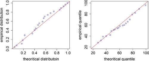
Table 3. Upper prediction limits (UPL) and upper tolerance limits (UTL) by predlimits and tollimits.

α	0.1	0.05	0.01
UPL	85.88	92.20	121.5
$(\gamma ,\alpha )$	(0.9,0.05)	(0.95, 0.05)	(0.99, 0.05)
UTL	97.67	110.1	138.0

5. Conclusion

This article introduces the gammadist package, which implements the up-to-date statistical methods for the gamma distribution. In specific, the rGamma function efficiently generates the gamma variates for all ranges of the parameter values, the parest function provides the closed-form estimators for the gamma parameters, and the conflimits, the predlimits, and the tollimits functions, respectively, construct the confidence limits, prediction limits, and tolerance limits with an accurate coverage for the gamma distribution. All these functions essentially deal with the fundamental statistical problems of applying the gamma distribution in practice. For each function, its associated methods have been introduced and its demo codes have been provided. A real environment monitoring application has demonstrated the usefulness of the package. The package is available on https://github.com/statcp/gammadist.

Further development of the package could focus on incorporating more functions related to the gamma distribution. For example, goodness-of-fit test of the gamma distribution is a premise to implement the model in practice. We show in Section 4 that the use of the parest function could be the first step to facilitate graphical assessments or some commonly used tests. Nevertheless, the uncertainties in the estimators may weaken the power of those tests. If more accurate and advanced methods of testing goodness-of-fit of the gamma distribution become available, they could be integrated to the gammadist package as a separate function. As another example, the three-parameter gamma distribution with an additional scale parameter is often used to fit lifetimes of products/units that cannot fail below a threshold (see, e.g., Ye, Hong, and Xie 2013). The rGamma function can be naturally extended to generate random variables from a three-parameter gamma distribution. However, estimation of parameters is a difficult research problem, let alone construction of the statistical limits. Substantial efforts are needed in order to include the three-parameter gamma distribution in our package. At last, the package may be further extended to deal with the gamma process, which is a commonly used stochastic model. Although the gamma distribution and the gamma process have a close relationship, some fundamental issues for the gamma process, such as accurate estimation and prediction, have not been completely addressed in the literature. The authors will pay special attention to the methodology development of the gamma process and are willing to enrich the gammadist package once these methods become available.

Acknowledgments

Authors are grateful to the editor, associate editor, and anonymous referees for the helpful comments regarding both the gammadist package and the preparation of this article.

Disclosure statement

No potential conflict of interest was reported by the authors.

Additional information

Funding

Zhao was supported in part by the National Natural Science Foundation of China under grant numbers 72002149 and 72032005.

Notes on contributors

Piao Chen

Piao Chen is an assistant professor in statistics at Delft Institute of Applied Mathematics, Delft University of Technology. He obtained his PhD in Industrial and Systems Engineering Management from National University of Singapore in 2017, and Bachelor in Industrial Engineering from Shanghai Jiao Tong University in 2013. His research interests include reliability engineering, quality management, and industry statistics. His work has appeared in journals including Technometrics, Journal of Quality Technology, Statistics in Medicine, Naval Research Logistics, IISE Transactions, European Journal of Operational Research, IEEE Transactions on Reliability, and Reliability Engineering & System Safety.

Kilian Buis

Kilian Buis is currently a master student at Delft Institute of Applied Mathematics, Delft University of Technology. He was a bachelor student under the supervision of Dr. Piao Chen.

Xiujie Zhao

Xiujie Zhao is an associate professor with the College of Management and Economics, Tianjin University, Tianjin, China. He received a BE degree from Tsinghua University, an MS degree from the Pennsylvania State University and a PhD degree from City University of Hong Kong, all in industrial engineering. His research interests include accelerated reliability testing, degradation modeling, maintenance optimization and design of experiments. His papers have appeared in IISE Transactions, European Journal of Operational Research, Journal of Quality Technology, IEEE Transactions on Reliability, Reliability Engineering & System Safety, among others.

Appendix:

R codes for real application

## Load package and alkalinity concentrations datalibrary(gammadist)x <- c(58,82,42,28,118,96,49,54,42,39,40,60,63,59,51,66,89,40,51,54,55,59,42,70,32,52,79)## Point estimates and confidence intervals of parametersest.all <- parest(x)est.shape <- est.all$shapeest.rate <- est.all$rateconf.all <- conflimits(x,alpha = 0.1)## Graphical goodness-of-fit test# compute the empirical cdfFn <- ecdf(x)# P-P plotplot(pgamma(x,est.shape,est.rate),Fn(x),col=’blue’,cex.main = 1.5,cex.lab = 1.5,cex.axis = 1.5,xlab=’theoritical distributoin’, ylab= ’empirical distribution’)abline(0,1,col = ’red’)# Q-Q plotplot(qgamma(Fn(x),est.shape,est.rate),x,xlim = c(20,100),ylim = c(20,100),col=’blue’,cex.main = 1.5,cex.lab = 1.5,cex.axis = 1.5,xlab=’theoritical quantile’,ylab=’empirical quantile’)abline(0,1,col=’red’)## K-S testks.test(x,"pgamma",est.shape,est.rate)## Upper prediction limitspredlimits(x,0.1)$pred[4]predlimits(x,0.05)$pred[4]predlimits(x,0.01)$pred[4]## Upper tolerance limitstollimits(x,0.05,0.9)$tol[4]tollimits(x,0.05,0.95)$tol[4]tollimits(x,0.05,0.99)$tol[4]

References

- Ahrens, J. H., and U. Dieter. 1974. Computer methods for sampling from gamma, beta, Poisson and bionomial distributions. Computing 12 (3):223–46. doi: 10.1007/BF02293108.
- Ahrens, J. H., and U. Dieter. 1982. Generating gamma variates by a modified rejection technique. Communications of the ACM 25 (1):47–54. doi: 10.1145/358315.358390.
- Al-Ahmadi, S., and H. Yanikomeroglu. 2010. On the approximation of the generalized-K distribution by a gamma distribution for modeling composite fading channels. IEEE Transactions on Wireless Communications 9 (2):706–13. doi: 10.1109/TWC.2010.02.081266.
- Baran, S., and D. Nemoda. 2016. Censored and shifted gamma distribution based EMOS model for probabilistic quantitative precipitation forecasting. Environmetrics 27 (5):280–92. doi: 10.1002/env.2391.
- Best, D. 1983. A note on gamma variate generators with shape parameter less than unity. Computing 30 (2):185–8. doi: 10.1007/BF02280789.
- Bhaumik, D. K., and R. D. Gibbons. 2006. One-sided approximate prediction intervals for at least p of m observations from a gamma population at each of r locations. Technometrics 48 (1):112–9. doi: 10.1198/004017005000000355.
- Bhaumik, D. K., K. Kapur, and R. D. Gibbons. 2009. Testing parameters of a gamma distribution for small samples. Technometrics 51 (3):326–34. doi: 10.1198/tech.2009.07038.
- Chen, P., and Z.-S. Ye. 2017a. Approximate statistical limits for a gamma distribution. Journal of Quality Technology 49 (1):64–77. doi: 10.1080/00224065.2017.11918185.
- Chen, P., and Z.-S. Ye. 2017b. Estimation of field reliability based on aggregate lifetime data. Technometrics 59 (1):115–25. doi: 10.1080/00401706.2015.1096827.
- Chen, P., and Z.-S. Ye. 2018. A systematic look at the gamma process capability indices. European Journal of Operational Research 265 (2):589–97. doi: 10.1016/j.ejor.2017.08.024.
- El-Zaart, A. 2010. Images thresholding using ISODATA technique with gamma distribution. Pattern Recognition and Image Analysis 20 (1):29–41. doi: 10.1134/S1054661810010037.
- Gao, G., K. Ouyang, Y. Luo, S. Liang, and S. Zhou. 2017. Scheme of parameter estimation for generalized gamma distribution and its application to ship detection in SAR images. IEEE Transactions on Geoscience and Remote Sensing 55 (3):1812–32. doi: 10.1109/TGRS.2016.2634862.
- Hannig, J., H. Iyer, and P. Patterson. 2006. Fiducial generalized confidence intervals. Journal of the American Statistical Association 101 (473):254–69. doi: 10.1198/016214505000000736.
- Hayter, A., and S. Kiatsupaibul. 2014. Exact inferences for a gamma distribution. Journal of Quality Technology 46 (2):140–9. doi: 10.1080/00224065.2014.11917959.
- Iliopoulos, G. 2016. Exact confidence intervals for the shape parameter of the gamma distribution. Journal of Statistical Computation and Simulation 86 (8):1635–42. doi: 10.1080/00949655.2015.1080705.
- Krishnamoorthy, K., M. Lee, and D. Zhang. 2017. Closed-form fiducial confidence intervals for some functions of independent binomial parameters with comparisons. Statistical Methods in Medical Research 26 (1):43–63. doi: 10.1177/0962280214537809.
- Krishnamoorthy, K., A. Mallick, and T. Mathew. 2011. Inference for the lognormal mean and quantiles based on samples with left and right type I censoring. Technometrics 53 (1):72–83. doi: 10.1198/TECH.2010.09189.
- Krishnamoorthy, K., and T. Mathew. 2009. Statistical tolerance regions: Theory, applications, and computation. Hoboken, New Jersey, United States: John Wiley & Sons.
- Krishnamoorthy, K., T. Mathew, and S. Mukherjee. 2008. Normal-based methods for a gamma distribution: Prediction and tolerance intervals and stress-strength reliability. Technometrics 50 (1):69–78. doi: 10.1198/004017007000000353.
- Krishnamoorthy, K., and X. Wang. 2016. Fiducial confidence limits and prediction limits for a gamma distribution: Censored and uncensored cases. Environmetrics 27 (8):479–493. doi: 10.1002/env.2408.
- Kundu, D., and R. D. Gupta. 2007. A convenient way of generating gamma random variables using generalized exponential distribution. Computational Statistics & Data Analysis 51 (6):2796–802. doi: 10.1016/j.csda.2006.09.037.
- Lee, C., and J. C. Wang. 2011. Waiting time probabilities in the M/G/1+ M queue. Statistica Neerlandica 65 (1):72–83. doi: 10.1111/j.1467-9574.2010.00476.x.
- Lin, Y.-W., and Y.-B. Lin. 2015. Mobile ticket dispenser system with waiting time prediction. IEEE Transactions on Vehicular Technology 64 (8):3689–96. doi: 10.1109/TVT.2014.2356644.
- Liu, C., R. Martin, and N. Syring. 2017. Efficient simulation from a gamma distribution with small shape parameter. Computational Statistics 32 (4):1767–75. doi: 10.1007/s00180-016-0692-0.
- Louzada, F., P. L. Ramos, and E. Ramos. 2019. A note on bias of closed-form estimators for the gamma distribution derived from likelihood equations. The American Statistician 73 (2):195–9. doi: 10.1080/00031305.2018.1513376.
- Marsaglia, G., and W. W. Tsang. 2000. A simple method for generating gamma variables. ACM Transactions on Mathematical Software 26 (3):363–72. doi: 10.1145/358407.358414.
- Wang, B. X., and F. Wu. 2018. Inference on the gamma distribution. Technometrics 60 (2):235–44. doi: 10.1080/00401706.2017.1328377.
- Wang, X., B. X. Wang, Y. Hong, and P. H. Jiang. 2021a. Degradation data analysis based on gamma process with random effects. European Journal of Operational Research 292 (3):1200–8. doi: 10.1016/j.ejor.2020.11.036.
- Wang, X., B. X. Wang, X. Pan, Y. Hu, Y. Chen, and J. Zhou. 2021b. Interval estimation for inverse Gaussian distribution. Quality and Reliability Engineering International 37 (5):2263–75. doi: 10.1002/qre.2856.
- Weerahandi, S. 1993. Generalized confidence intervals. Journal of the American Statistical Association 88 (423):899–905. doi: 10.1080/01621459.1993.10476355.
- Xi, B., K. M. Tan, and C. Liu. 2013. Logarithmic transformation-based gamma random number generators. Journal of Statistical Software 55 (4):1–17. doi: 10.18637/jss.v055.i04.
- Xiao, X., P. Chen, Z. Ye, and K.-L. Tsui. 2021. On computing multiple change points for the gamma distribution. Journal of Quality Technology 53 (3):267–88. doi: 10.1080/00224065.2020.1717398.
- Ye, Z.-S., and N. Chen. 2017. Closed-form estimators for the gamma distribution derived from likelihood equations. The American Statistician 71 (2):177–81. doi: 10.1080/00031305.2016.1209129.
- Ye, Z.-S., Y. Hong, and Y. Xie. 2013. How do heterogeneities in operating environments affect field failure predictions and test planning? The Annals of Applied Statistics 7 (4):2249–71. doi: 10.1214/13-AOAS666.