Freezing point depression in model Lennard-Jones solutions

Abstract

Crystallisation of liquid solutions is of uttermost importance in a wide variety of processes in materials, atmospheric and food science. Depending on the type and concentration of solutes the freezing point shifts, thus allowing control on the thermodynamics of complex fluids. Here we investigate the basic principles of solute-induced freezing point depression by computing the melting temperature of a Lennard-Jones fluid with low concentrations of solutes, by means of equilibrium molecular dynamics simulations. The effect of solvophilic and weakly solvophobic solutes at low concentrations is analysed, scanning systematically the size and the concentration. We identify the range of parameters that produce deviations from the linear dependence of the freezing point on the molal concentration of solutes, expected for ideal solutions. Our simulations allow us also to link the shifts in coexistence temperature to the microscopic structure of the solutions.

Keywords:

• Lennard-Jones
• solution
• melting temperature
• molecular dynamics

1. Introduction

Thermodynamics and kinetics of solid–liquid phase transitions rule several processes that have a massive impact on life on Earth. Freezing and melting of water and aqueous solutions deeply influence climate, atmospheric and geological processes, materials processing and food processing and conservation. At a given pressure, crystallisation and melting rates are controlled in first instance by the temperature at which the liquid and the solid phase coexist in equilibrium, i.e. the coexistence temperature (T _c ). Even though T _c is an intrinsic property of materials, it can be affected by external factors, for example by the high curvature of capillary walls [1] under micro or nano-confinement [2], by the confinement length [3] or by the presence of impurities, even at very low concentration [4,5].

In solutions, T _c is usually reduced by an amount proportional to the solute concentration. This is commonly experienced, for example, when ice is molten at temperatures lower than 0°C by adding salt. In the ideal case of a binary system, in which the solute is fully diluted, the depression of the coexistence temperature, $\Delta T_c=T_c^{\text{solution}}-T_c^{\text{pure}\text{solvent}}$, depends linearly on the molality m of the solute, with a proportionality constant k. In aqueous solutions, k is a dubbed cryoscopic constant. In the ideal case, k does not depend on the type of solute but only on its concentration, so that (1) $$\Delta T_c=-k·m.$$(1) The basic rationale behind such ideal behaviour is that the addition of solute to a pure solvent increases the entropy of the solution by an amount proportional only to the number of added solute particles, independently on the chemical nature of the solute [6]. The excess entropy shifts the phase balance between liquid and solid in favour of the liquid, thus shifting the T _c . The simplicity and universality of this relation is exploited to measure the vapour pressure of solutions of electrolytes and/or their molar number [7,8].

However, Equation (1(1) $$\Delta T_c=-k·m.$$(1) ) is only justified in the case of an ideal dilution, that is at very low solute concentrations, and it was observed to break down already for 0.5 molal aqueous solutions [9]. Deviations from ideal behavior stem from specific molecular interactions, namely solute–solute, solvent–solute interactions, and solute-induced variations in solvent–solvent interactions [10]. At low concentration, solvent–solute interactions are expected to play the most important role, and empirical corrections to the ideal freezing point depression law have been devised in terms of solute–solvent interaction or activity coefficients [10–12]. Equation (1(1) $$\Delta T_c=-k·m.$$(1) ) can be generalised to take into account deviations from the linear behaviour due to the partial dissociation of solutes, by including the Van't Hoff dissociation factor i, so that (2) $$\Delta T_c=-i·k·m.$$(2) Even if empirical models may result successful for specific cases a microscopic theory linking the thermodynamics of solid–liquid phase transitions of binary solutions to their structural properties islacking.

In this work, we verify to what extent Equation (1(1) $$\Delta T_c=-k·m.$$(1) ) holds for a simple system, and provide the missing link between the shift in the coexistence temperature and the structural changes in the solvent, induced by the presence of different types of solutes. We especially want to target the conditions often occurring in biological environments or in food processing, in which the presence of few large macromolecules produces significant shifts in the coexistence temperature of water. To this scope, we employ molecular dynamics (MD) simulations on model systems, consisting of binary Lennard-Jones (LJ) mixtures, in which one of the two components, made of larger particles, is kept at low concentration (<2.5% in number of particles) and acts as solute, and the other acts as solvent.

LJ mixtures are valuable models to understand the general features of crystallisation in binary solutions, from nucleation [13] to growth [14–17]. More complex LJ mixtures with suitably chosen interaction parameters were also used to model how additives modulate the nucleation and crystal growth of solutes in supersaturated solutions [18,19]. The phase diagram of binary LJ mixtures was extensively characterised in former works [20–22]. Nevertheless, these works take into account mixtures of particles with rather similar size (diameter ratio up to ∼1.2), and do not discuss the effect of large solute particles at small concentrations on the solid–liquid transition temperature of a solvent made of smaller LJ particles, which, instead, is the focus of this work.

Two types of solute–solvent interaction and a broad range of sizes and concentrations of solute particles are tested. We show that ΔT _c deviates significantly from the ideal behaviour in Equation (1(1) $$\Delta T_c=-k·m.$$(1) ) for solutes smaller than a certain size even at very low concentrations, while the effect of larger solutes on T _c is correctly predicted. We then propose a link between ΔT _c and how solutes modify the short- and medium-range order of the solvent, probed by computing the static structure factor S(k) and the excess configurational entropy.

2. Models and numerical methods

We compute the melting temperature of a binary LJ mixture by MD simulations. Solid–liquid phase transitions in single-component LJ are well characterised: the solid–liquid phase coexistence line was computed by Agrawal and Kofke [23], and several studies investigated nucleation from the melt [24–27] and crystal growth [28,29].

In our simulations of LJ binary mixtures, the interaction between two particles of type a and b at distance r is described by the truncated and shifted LJ potential [30], (3) $$V_{ab}\left(r\right)=\left\{\begin{array}{cc}\hfill v_{ab}\left(r\right)-v_{ab}\left(r^c\right),& \hfill \text{if}{r}_{ab}<r^c,\\ \hfill 0,& \hfill \text{otherwise},\end{array}\right.$$(3) where (4) $$v_{ab}\left(r\right)=4{ϵ}_{ab}\left[{\left(\frac{{\sigma }_{ab}}{r}\right)}^{12}-{\left(\frac{{\sigma }_{ab}}{r}\right)}^6\right].$$(4) We define type-1 particles as solvent and type-2 particles as solute (at low concentration), and σ₁₁ = 1 and ϵ₁₁ = 1 as length and energy units. All particles have unitary mass and all the other quantities are expressed in reduced units derived from σ₁₁ and ϵ₁₁. For example, time is expressed in $\tau ={\sigma }_{11}\sqrt{m/{ϵ}_{11}}$ and pressure in ϵ₁₁/σ³ ₁₁. The interaction parameters between mixed species ϵ₁₂ and σ₁₂, are defined as geometric averages ${ϵ}_{12}=\sqrt{{ϵ}_{11}{ϵ}_{22}}$ and ${\sigma }_{12}=\sqrt{{\sigma }_{11}{\sigma }_{22}}$. Interactions are truncated at a cut-off r ^c = 3.7 and long-range corrections to potential energy and pressure are applied to compensate the effect of truncation to the LJ equation of state [31]. A so large r ^c is necessary to account correctly for the interactions, when σ₂₂ is much larger than 1.

The direct calculation of the coexistence temperature T _c by either heating a crystal until it melts or cooling a liquid until it freezes would be affected by large hysteresis, due to the finite size of the simulation cell and the presence of the nucleation barrier. To circumvent this issue, we adopt the two-phase method [32], which allows an accurate and direct evaluation of T _c at a given pressure in a single simulation. This approach consists of simulating a crystal in contact with its melt in the same simulation cell with periodic boundary conditions (Figure 1). After equilibration at a chosen temperature, the system with a fixed number of particles N is allowed to evolve at constant pressure and constant enthalpy (NPH). In the NPH ensemble, one of the two phases, depending on the initial temperature, grows at the expenses of the other producing or adsorbing latent heat and the system evolves spontaneously towards the coexistence temperature. Provided that the size of the system is sufficiently large to avoid interactions between solid–liquid interfaces, the T _c obtained by this approach is in excellent agreement with that computed by the thermodynamic integration [33].

Figure 1. Example of a simulation setup for solutes with size σ₂₂ = 1.5 at 1% number concentration. The z-direction is perpendicular to the interface seen roughly in the middle of the box. Particles in the liquid phase are on the right part of the box and host the solute particles with diameter size σ₂₂ (shown in green). All particles shown in light blue have size σ₁₁ = 1.0.

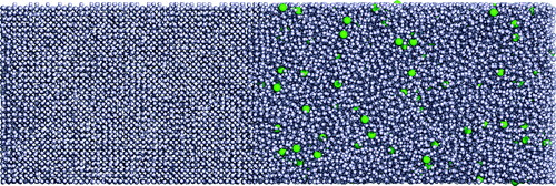
The starting configuration, with dimension 25 × 25 × 85, containing about 45 · 10³ particles, was equilibrated using the Berendsen thermostat and barostat [34] at the melting temperature of the single component system, $T_c^{\text{pure}}=0.694\left(1\right)$, at a pressure of 0.002387 ϵ₁₁/σ³ ₁₁. The NPH ensemble is enforced by using the Parrinello–Rahman barostat [35], an extension to non-isotropic cell deformation of the Andersen barostat [36]. This algorithm is based on an extended Hamiltonian, in which the cell parameters are additional dynamical variables, and its conserved quantity is the total enthalpy. The pressure is controlled by using a barostat coupling parameter τ _p = 30 and the default compressibility, κ _T = 0.021, and the angles of the simulation box are constrained. The systems consist of a solid bock made of type-1 (solvent) particles, and a liquid phase containing also type-2 solute particles at the number concentration $c=N_{\text{solutes}}/N_{\text{solvent}}^{\text{liq}}$, where $N_{\text{solvent}}^{\text{liq}}$ is the number of solvent particles in the liquid state. Note, that with this definition and choice of mass m = 1, the molality m = n _solute/m _solvent is equivalent to the number concentration c. We consider both solvophilic (ϵ₁₁ = ϵ₁₂ = ϵ₂₂ = 1) and weakly solvophobic (ϵ₁₂ = ϵ₁₁/2 = 0.5 and ϵ₂₂ = 0.25) solutes with size σ₂₂ between 1.1 and 2.5 at number concentration c between 0.1% and 2.5%.

MD simulations are performed using GROMACS [37] and the equations of motion are integrated with a timestep Δt = 0.005. Production runs in which thermodynamic averages are calculated are 4 × 10⁵ steps long, resulting in 2000τ long trajectories. Five independent runs for each parameter pair (size, initial concentration) were carried out. During the NPH simulation, the number of particles in the liquid state changed due to the phase transition. In order to obtain the final concentration of the system, the number of particles in the liquid state was averaged over the last 100 frames (starting at t = 1500 τ in steps of 5) and the concentration computed to c = (number of solutes/average number of solvent particles). Taking the mean value (along with the standard deviation) of all five runs leads to the final result for a given solute parameter pair. The melting temperature was obtained by averaging over the last 500 τ of each independent trajectory.

To determine which solvent particles are in either the liquid or the solid phase, we use Steinhardt's order parameter [38] modified by Wolde [39]. We calculate for each solvent particle i, the complex vector q _6m (i) as follows: for each neighbour j = 1…N _b (i) of particle i, where N _b (i) is the total number of neighbours around i within a chosen cut-off range (we chose the first minimum in the radial distribution function), calculate (5) $$\begin{array}{c}\hfill {\tilde{q}}_{6m}\left(i\right)=\frac{1}{N_b\left(i\right)}\sum _{j=1}^{N_b\left(i\right)}{Y}_{6m}\left({\widehat{\mathbf{r}}}_{ij}\right),\end{array}$$(5) where ${\widehat{\mathbf{r}}}_{ij}$ is the normalised distance vector between i and j and $Y_{6m}\left({\widehat{\mathbf{r}}}_{ij}\right)$ are spherical harmonics of angular momentum l = 6. The sum of the normalised scalar products leads to q ₆(i), (6) $$\begin{array}{c}\hfill q_6\left(i\right)=\sum _{j=1}^{N_b\left(i\right)}\frac{{\sum }_{m=-6}^6{\tilde{q}}_{6m}\left(i\right){\tilde{q}}_{6m}^{*}\left(j\right)}{{\left({\sum }_{m=-6}^6{\left|{\tilde{q}}_{6m}\left(i\right)\right|}^2\right)}^{{}^1{/}_2}{\left({\sum }_{m=-6}^6{\left|{\tilde{q}}_{6m}\left(j\right)\right|}^2\right)}^{{}^1{/}_2}},\end{array}$$(6) and quantifies the symmetry around particle i. If this value is greater than 0.7, the particle is identified as crystalline. The local order parameter q ₆ has proven to work particularly well for the expected face-centred-cubic symmetry in LJ systems [25].

We also performed microcanoncial MD simulations to analyse the structure and thermodynamics of liquid solutions in a simulation box containing about 22 · 10³ particles. Specifically, we computed the radial distribution function g ₁₁(r) of the solvent and the static structure factor S ₁₁(k). Hereon for the sake of simplicity, we refer S ₁₁(k) and g ₁₁(r) as S(k) and g(r). S(k) is calculated as the Fourier transform of g(r): (7) $$S\left(\mathrm{k}\right)=1+\frac{4\pi \rho }{\mathrm{k}}\int dr(g\left(r\right)-1)rsin\left(\mathrm{k}r\right).$$(7) We calculated the conformational entropy $\left(\mathcal{S}\right)$ of the solvent using the excess entropy formalism [40,41]. The total thermodynamic entropy is the sum of the ideal gas entropy ${\mathcal{S}}_{\text{id}}$ and the excess entropy ${\mathcal{S}}_e$, (8) $$\mathcal{S}={\mathcal{S}}_{\text{id}}+{\mathcal{S}}_e.$$(8) The entropy of an ideal gas reads (9) $${\mathcal{S}}_{\text{id}}/N{k}_B=ln\left(\frac{V}{N{\lambda }^3}\right)+\frac{5}{2},$$(9) where N is the number of particles of the system, V the volume, k _B the Boltzmann constant, β the inverse temperature, h the Planck constant and λ the de Broglie wavelength, $\lambda =h\sqrt{\beta /2\pi m}$. The excess entropy is expressed as a multiparticle correlation expansion [40,41], (10) $${\mathcal{S}}_e={\mathcal{S}}_2+{\mathcal{S}}_3+\cdots \text{,}$$(10) with ${\mathcal{S}}_n$ as the n-particle correlation contribution. ${\mathcal{S}}_2$, the contribution due to pair correlations between atoms of the same type, can be calculated from the pair distribution function as follows: (11) $${\mathcal{S}}_2/N{k}_B=-2\pi \rho \underset{0}{\overset{R_{\text{max}}}{\int }}dr\left\{g\left(r\right)lng\left(r\right)-\left[g\left(r\right)-1\right]\right\}{r}^2,$$(11) where the integral is computed from 0 to a radius R _max at which g(R _max) ≃ 1. Our expansion of the excess entropy is truncated after the pair wise term ${\mathcal{S}}_2$. The calculation of $\mathcal{S}$ is carried out taking into account the solvent only, therefore the quantities N, g(r) and ρ refer solely to type-1 particles.

Solutes in the binary LJ mixture start to form clusters with increasing solute size and concentration depending on the solute–solvent and solute–solute interactions. The amount of clusters, or the affinity to form clusters, is computed by using a clustering order parameter Φ, defined as (12) $$\Phi =\frac{\text{number}\text{of}\text{clusters}}{\text{number}\text{of}\text{solutes}}.$$(12) The clusters in the liquid mixture are identified and counted using a nearest-neighbour criterion. For each solute particle, all neighbouring solute particles within a cut-off corresponding to the first minimum in the radial distribution function g ₂₂(r) are recursively marked as belonging to the same cluster.

3. Results and discussion

3.1. Freezing-point depression

The proportionality constant in Equation (1(1) $$\Delta T_c=-k·m.$$(1) ) for an ideal solution is given by [42]: (13) $$\begin{array}{c}\hfill k=R{T}_c^2/\Delta H,\end{array}$$(13) where ΔH is the enthalpy difference between the solid and the liquid phase. The melting enthalpy per particle for our system at P = 0.002387 ϵ₁₁/σ³ ₁₁ is ΔH = 1.12467 ϵ₁₁, in agreement with the previous calculations at similar conditions [31,43]. At T _c = 0.694(1) with the gas constant in reduced units, R = 8.3473 · 10⁻³/K, k for an ideal solution in reduced units at the thermodynamic conditions considered here is 3.575(8) · 10⁻³.

Figure 2. ΔT _c as a function of the concentration of solvophilic solutes with diameter sizes σ₂₂ = 1.1 and σ₂₂ = 2.0. The data points are shown along with the weighted linear fit. The resulting negative slopes are 0.0011(6)T _c and 0.0049(3)T _c (or 0.7(4) 10⁻³ and 3.4(2) 10⁻³ in reduced units) for systems with solvophilic solute sizes σ₂₂ = 1.1 and σ₂₂ = 2.0, respectively. The coexistence temperature T _c was computed for the pure Lennard-Jones solvent to T _c = 0.694(1). Considering the differences in some simulation parameters, e.g. the interaction cut-off and the size of the system, this result agrees well with the result obtained from the thermodynamic integration by Agrawal and Kofke [23], T _c = 0.687(4).

Using the two-phase approach, we compute the melting temperature for the LJ binary mixtures described in the previous section. We found that the expected linear dependence of ΔT _c on the number, or equivalently molal, concentration in Equation (1(1) $$\Delta T_c=-k·m.$$(1) ) is retrieved for all the considered solvophilic solutes. Examples are shown in Figure 2, in which we plot ΔT _c as a function of concentration of solvophilic solutes of two different sizes. The figure clearly shows that the slope of the linear fit is not independent on the size of the solute particles, as predicted by the ideal solvation model, but varies from 0.0003(1) to 0.0039(2). We can already argue that these systems deviate from the ideal behaviour, with the consequence that k is not solely a colligative property of the solvent. Hence, we will call the proportionality factor in Equation (1(1) $$\Delta T_c=-k·m.$$(1) ) α(σ₂₂) to avoid confusion with the theory of fully diluted systems. It is then worth computing systematically the proportionality factor α(σ₂₂) as a function of the size and the interaction type of solutes, as shown in Figure 3.

Figure 3. Proportionality factor α between the solute concentration and ΔT _c as a function of solute size σ₂₂. α(σ₂₂) was obtained from linearly fitting ΔT _c (c) for different σ₂₂. The standard deviation of the fit quantifies the error bars of α(σ₂₂). (a) Solvophilic solutes with ϵ₂₂ = 1.0. (b) Weakly solvophobic solutes with ϵ₂₂ = 0.25. The grey line marks the value of the cryoscopic constant of an ideal Lennard-Jones solution, the dashed line in (a) indicates the average proportionality factor considering the data collected for σ₂₂ between 1.3 and 2.0.

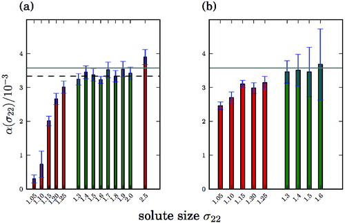
For solvophilic solutes (Figure 3(a)), for sizes σ₂₂ ≥ 1.3, the proportionality factor α in ΔT _c (c) does not depend on σ₂₂ within error bars and is fairly close to the k predicted by theory (solid line in Figure 3). On the other hand, for σ₂₂ ≤ 1.25, α(σ₂₂), is much smaller. α(σ₂₂) increases with σ₂₂ and saturates at a plateau for 1.3 ≤ σ₂₂ ≤ 2.0 at α ≈ 0.00334(4), 7% below the theoretical value for the cryoscopic constant calculated from Equation (13(13) $$\begin{array}{c}\hfill k=R{T}_c^2/\Delta H,\end{array}$$(13) ).

The resulting proportionality factors α(σ₂₂) for weakly solvophobic solutes are reported in Figure 3(b). α(σ₂₂) slowly increases with σ₂₂ up to 1.3 and stays constant up to σ₂₂ = 1.6. Overall, the proportionality factor α(σ₂₂) varies from 0.0025(1) to 0.0037(11) and the dependence of α on σ₂₂ is less pronounced than for solvophilic solutes. The results for weakly solvophobic solutes with ϵ₂₂ = 0.25 require a more differentiated analysis.

The linear dependence of ΔT _c on the entire concentration range of c up to 2.5% is observed only for solutes with sizes σ₂₂ ≤ 1.3. For larger solutes, ΔT _c is proportional to c only up to a threshold concentration c ^max. The reason is that at c ≥ c ^max, the solutes start to cluster and one should correct the definition of number concentration taking into account such effect. Thus, for weakly solvophobic solutes with size σ₂₂ between 1.3 and 1.6, the slope α(σ₂₂) was obtained from a linear fit up to c ^max. Larger solutes, σ₂₂ ≥ 1.7, form clusters even at very low concentrations, making it impossible to estimate α(σ₂₂). The maximum concentration c ^max was defined by a threshold value of the clustering order parameter Φ of Equation (12(12) $$\Phi =\frac{\text{number}\text{of}\text{clusters}}{\text{number}\text{of}\text{solutes}}.$$(12) ). With increasing solute size and concentration, weakly solvophobic solutes form more clusters and Φ decreases. At Φ ≈ 80%, the linear dependence of ΔT _c on c breaks down and, depending on the solute size, determines the maximum concentration c ^max. The maximum freezing point depression obtained for weakly solvophobic solutes (1.03%) in the range of concentrations considered here is significantly lower than that calculated for solvophilic solutes, with σ₂₂ = 2.5, at the concentration of 2.3%, thus indicating that large solvophilic particles can be used more effectively to control the thermodynamics of phase transitions of solutions. In fact, weakly solvophobic solutes depress T _c as efficiently as solvophilic solutes only in the low concentration range, when clustering is avoided. On the other hand, when solutes begin to cluster, the freezing temperature of the solution stops decreasing and becomes independent on the concentration of solute particles, as shown in Figure 4, where ΔT _c (c) is plotted together with the clustering order parameter Φ.

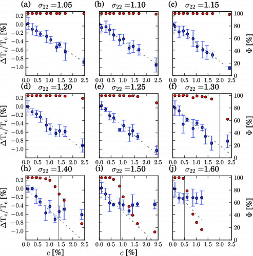
Figure 4. ΔT _c (c) for weakly solvophobic solutes with different sizes σ₂₂. The blue data points show the freezing-point depression. The dashed line is the resulting fit of the linear model of Equation (1(1) $$\Delta T_c=-k·m.$$(1) ). The slopes of the fits lead to the results shown in Figure 3. With increasing solute size, the linear regime breaks down at lower concentrations, which is indicated by the vertical grey line. The red points represent the clustering order parameter with Φ = 100% as the fully dispersed state and Φ = 0% as the fully phase segregated state. The linear regime of ΔT _c holds up to Φ = 80%.

In general, our results show that in contrast with the theory for ideal solutions, size and interaction type of the solute particles affect the freezing-point depression. Deviations from the ideal behaviour expressed in Equation (1(1) $$\Delta T_c=-k·m.$$(1) ) need to be analysed in detail.

3.2. Entropy corrections for solid state solution

For ‘small’ solute particles, we observe a significant reduction of proportionality factors α(σ₂₂) with respect to the ideal cryoscopic constant k. The origin of such deviations from the ideal behaviour is that in deriving Equation (13(13) $$\begin{array}{c}\hfill k=R{T}_c^2/\Delta H,\end{array}$$(13) ), one ignores the possibility that incorporating solutes in the crystal to form a solid solution may be thermodynamically favourable. In fact, when solutes are sufficiently small, we have to consider also how the Gibbs free energy of the solid phase changes upon incorporation of solute particles. We calculate the change of the free energy ΔG when changing single component crystal of N LJ particles to a solid solution made of N ₁ = N − N ₂ solvent particles and N ₂ solute particles, at constant temperature and pressure. Here we consider solvophilic solutes, both for the sake of simplicity and because incorporation is more effective in this case. The difference in the free energy of a pure solid solvent and a solid solution is $\Delta G=\Delta U-T\Delta \mathcal{S}+P\Delta V$, where U is the internal energy and $\mathcal{S}$ the entropy of the system. We neglect the relatively small volume term PΔV, and compute ΔU in a 24,576 particles system at coexistence. To improve the statistics, a set of different number of solutes, $$\begin{array}{c}\hfill \left\{N_2\right\}=\{122,147,171,195,219,243,303,363,482\}\end{array}$$was probed. For solutes with a large σ₂₂, a smaller subset of {N ₂} was used because of equilibration issues for large N ₂.

While the energy difference is computed by MD, the difference in entropy, $\Delta \mathcal{S}={\mathcal{S}}^{\text{ss}}-{\mathcal{S}}^{\text{sc}}$ is derived as follows. To get the configurational entropy of the solid solution ${\mathcal{S}}^{\text{ss}}$, we consider N crystal lattice sites and replace N ₂ of them with solute particles. The number of configurations Ω is (14) $$\begin{array}{ccc}\hfill \Omega =\left(\begin{array}{c}N\\ N_2\end{array}\right)& =& \frac{N!}{N_1!N_2!}.\hfill \end{array}$$(14) With $\mathcal{S}=k_{B}ln\left(\Omega \right),$ we find for the entropy ${\mathcal{S}}^{\text{ss}}$ (15) $$\begin{array}{ccc}\hfill {\mathcal{S}}^{\text{ss}}& =& -k_B\left[lnN!-ln{N}_2!-ln{N}_1!\right]\hfill \end{array}$$(15) (16) $$\begin{array}{ccc}& =& -k_{B}N\left[ln\left(1-x_2\right)+x_{2}ln\left(\frac{x_2}{1-x_2}\right)\right],\hfill \end{array}$$(16) where we used Stirling's approximation and x ₂ = N ₂/N. Since the configurational entropy of the single component crystal is zero, $\Delta \mathcal{S}={\mathcal{S}}^{\text{ss}}$.

The entropy gain in solid solution $\Delta \mathcal{S}$ counteracts the difference in internal energy ΔU, making the solid solution thermodynamically more favourable than the single component crystal for solutes smaller than ∼1.18, as it is shown in Figure 5, which displays ΔG as a function of solute size.

Figure 5. Difference in the Gibbs free energy ΔG between a single component crystal and a solid solution for a 24576 particles system as a function of solute size σ₂₂ for different concentrations x ₂ = N ₂/N.

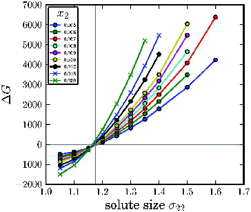
This shift in the reference free energy of the solid phase leads to deviations of the proportionality constant α from the ideal behaviour for σ₂₂ < 1.3 for solvophilic solutes. Also for solute sizes σ₂₂ ≥ 1.18, although less likely, incorporation in the solid phase is thermodynamically competitive.

3.3. Clustering of weakly solvophobic solute particles

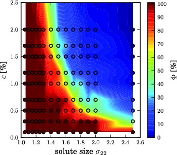
Weakly solvophobic solutes tend to cluster with increasing solute size and concentration. Clustering produces large deviations from the ideal freezing point depression behaviour. Here we analyse clustering of solute particles quantitatively. In Figure 6, the clustering order parameter Φ, computed from Equation (12(12) $$\Phi =\frac{\text{number}\text{of}\text{clusters}}{\text{number}\text{of}\text{solutes}}.$$(12) ), is plotted as a function of solute size σ₂₂ and concentration c. The figure shows that weakly solvophobic solutes stay dispersed if their size is close to the solvent particle size (σ₂₂ = 1.0), but start to cluster at σ₂₂ = 1.5 for c > 1.0%, often resulting in a completely phase-separated system. Solvophilic solutes stay dispersed over the entire concentration range considered. The two consequences of clustering are (1) saturation ΔT _c as a function of concentration, which hinders the calculation of the proportionality factors α(σ₂₂) for solutes with large σ₂₂, (2) less effective depression of T _c .

Figure 6. Clustering of the solution of weakly solvophobic solutes. The cluster ratio Φ is shown as a function of solute size σ₂₂ and concentration c. Φ = 100% is obtained for a fully dispersed system, Φ = 0% if the system is completely phase-separated. See Equation (12(12) $$\Phi =\frac{\text{number}\text{of}\text{clusters}}{\text{number}\text{of}\text{solutes}}.$$(12) ) for the definition of Φ. These results are determined by MD simulations in the microcanonical NVE ensemble of a liquid system of ≈22 · 10³ particles in a periodic supercell.

Comparing the clustering order parameter and the dependence of ΔT _c on the concentration of solvophobic solutes (Figure 4), for all solute sizes we find that a breakdown of the linear regime and saturation of ΔT _c occurs for Φ ∼ 80%. Therefore, we can conclude that Φ ∼ 80% dictates the threshold concentration at which a the maximum ΔT _c is attained for a given solute size. Remarkably, rescaling the concentration on the x-axis to $\tilde{c}$ based on either the Van't Hoff factor as in Equation (2(2) $$\Delta T_c=-i·k·m.$$(2) ) or the number of clusters as obtained from the clustering analysis does not restore a linear dependence of ΔT _c on $\tilde{c}$.

We need to point out that our simulations have been performed on finite periodic systems, and those with the highest degree of clustering tend to phase separate. However, phase separation does not occur over the simulated time scales, therefore we are actually probing out-of-equilibrium cases, which often occur in materials growth and food processing, as well as in the atmosphere.

3.4. Static structure factor and configurational entropy

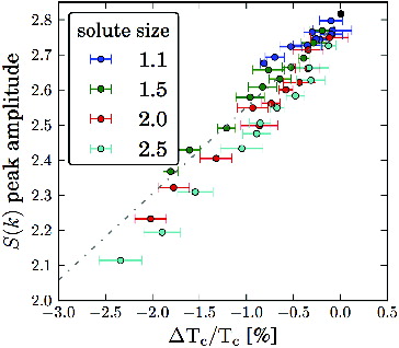
After discussing the deviations from the ideal behaviour of the freezing point depression, we now aim at establishing a direct link between the thermodynamic of the liquid–solid transition in solutions and the changes in the microscopic structure of the solvent upon insertion of solutes. In a seminal paper for the whole field of MD simulations, Hansen and Verlet demonstrated that a LJ liquid crystallises when the first peak of the structure factor S(k) is about 2.85 [31]. It is then reasonable to expect a correlation between the melting temperature of solutions and the amplitude of the first peak of the S(k) of the solvent. In our simulations, the amplitude of the first peak of the S(k) of the pure solvent at T _c is ∼2.81, in agreement with more recent estimates for liquids with various interaction potentials and for colloidal particles [44,45]. To probe such correlation, we computed the S(k) of binary LJ solutions in the microcanonical (NVE) ensemble, after equilibrating the systems at the melting temperature of the pure solvent. We considered both solvophilic and weakly solvophobic solutes of four different sizes (1.1, 1.5, 2 and 2.5 σ) over the whole range of concentrations up to 2.5%. Figure 7 shows that the amplitude of the first peak of the structure factor and the melting temperature of the solutions are indeed unmistakingly correlated, confirming that the mid-range structural modifications induced by the presence of solutes dictate the thermodynamics of phase transitions in solutions. The plot, however, does not include systems that tend to cluster and phase separate (Φ < 80%), for which the calculation of the S(k) is made problematic by size effects and by the out-of-equilibrium state of these systems.

Figure 7. Amplitude of the first peak of the static structure factor S(k) of the solvent upon insertion of solvophilic solutes of various size at different concentration, at the coexistence temperature of the pure system as a function of ΔT _c . The reference point of the pure system is a black circle. The fit (dashed grey line) has a Pearson correlation coefficient of 0.95, which indicates a solid linear dependence.

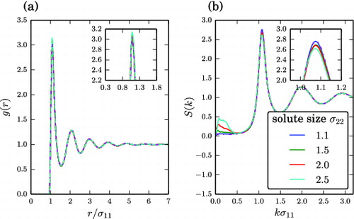
While this scenario may be compatible with the basic assumptions of the thermodynamics of freezing point depression in ideal solutions, we find that also systems with non-ideal freezing-point depression proportionality factor fall well within this general trend, and obey the Hansen–Verlet criterion. In fact, the changes in the amplitude of the first peak of the S(k) do not depend solely on the concentration but also on the size and the type of interaction of the solute particles. This fact can be appreciated in Figure 8, in which the S(k) of solutions contain four different solutes, all at the same concentration (1%). The amplitude of the first peak of the S(k) is indeed higher for the σ₂₂ = 1.1 solute and lower for the σ₂₂ = 2.5 solute, reflecting the different ability of different solutes to inhibit freezing, as formerly reported in Figure 3. No further significant changes appear in either the radial distribution function or the S(k), except for a peak arising at very small wavevector. The latter peak is an indicator of a long-range structure in the solute, possibly affected by the limited size of the simulated systems.

Figure 8. Results for the liquid mixtures with solvophilic solutes. (a) Radial distribution function g(r) of the solvent. The g(r) appears rather insensitive in the presence of different solutes, indicating that solutes do not affect the short-range structure of the solvent. The pure solvent reference system is represented by the purple dashed-dotted line. (b) Static structure factor S(k) of the solvent for different solute sizes. S(k) was computed according to Equation (7(7) $$S\left(\mathrm{k}\right)=1+\frac{4\pi \rho }{\mathrm{k}}\int dr(g\left(r\right)-1)rsin\left(\mathrm{k}r\right).$$(7) ). The system size varied from 21,120 to 23,113 particles at a fixed solute concentration of 1.0%. The insets show a magnification of the regions around the peaks. The pure solvent reference system is represented by the purple dashed-dotted line. Simulations are performed at the coexistence temperature of the pure solvent.

The amplitude of the first peak in the static structure factor S(k) is sensitive to medium-range structural disorder, and is a qualitative indicator of the configurational entropy of a liquid. The entropy $\mathcal{S}$ of the solvent is the dominating factor among the thermodynamic contributions to the free energy and is the leading influence on ΔT _c . A quantitative relation between structure and configurational entropy is given by the definition of the excess entropy ${\mathcal{S}}_e$, as the integral of the radial distribution function [40,41,46]. ${\mathcal{S}}_e$ computed according to Equation (11(11) $${\mathcal{S}}_2/N{k}_B=-2\pi \rho \underset{0}{\overset{R_{\text{max}}}{\int }}dr\left\{g\left(r\right)lng\left(r\right)-\left[g\left(r\right)-1\right]\right\}{r}^2,$$(11) ), is a pairwise addition to the entropy of the ideal gas, which depends on the density of the liquid as in Equation (9(9) $${\mathcal{S}}_{\text{id}}/N{k}_B=ln\left(\frac{V}{N{\lambda }^3}\right)+\frac{5}{2},$$(9) ). 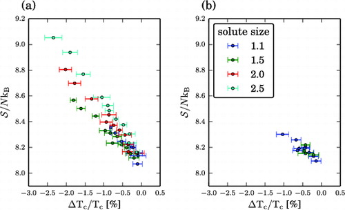The truncation to the pairwise term leads to a systematic overestimate of $\mathcal{S}$, which is relatively small at temperatures near the melting point. For example, this error was estimated about 2% for liquid sodium [40]. The entropy thus computed also correlates linearly with ΔT _c , especially for solvophilic solutes, as shown in Figure 9. Finite size and equilibration issues, related to the tendency to phase separate of weakly solvophobic solutes with σ₂₂ > 1.5, hinder the calculation of ${\mathcal{S}}_e$, yielding too large uncertainties.

Figure 9. Results for the liquid mixtures. Entropy $\mathcal{S}/N{k}_B$ as a function of ΔT _c . $\mathcal{S}$ was obtained according to Equation (8(8) $$\mathcal{S}={\mathcal{S}}_{\text{id}}+{\mathcal{S}}_e.$$(8) ), truncated after the pairwise term in the expansion of ${\mathcal{S}}_e$ and based on the g(r) of the solvent. (a) Solvophilic solutes. (b) Weakly solvophobic solutes. Shown are only the results for well-dispersed solutes, i.e. with a clustering value of Φ ≥ 80%.

4. Conclusions

In summary, utilising MD simulations of two-phase systems, we have investigated the freezing-point depression in model LJ solutions with fairly low concentration of solutes of varying size and two different types of interactions with the solvent, solvophilic and weakly solvophobic. Our results confirm that ΔT _c depends linearly on the molal concentration of the solute, as expected for ideal solutions at the limit of infinite dilution, as long as the solute does not tend to cluster and phase separate. We found that when the dispersion of the solute gets smaller than 80% increasing the molal concentration does not affect the freezing temperature of the solution. For this reasons, solvophilic solutes are more efficient to shift T _c . In addition, in the range of sizes and concentrations of solutes in which ΔT _c is proportional to the molal/number concentration, the proportionality constant is different from the ideal cryoscopic constant, and exhibits a dependence on the size of the solutes and the type of interaction of solutes–solvent interaction. Our analysis supports the classical picture based on the application of Raoult's law on ideal solutions, in which the presence of solutes shifts the free energy of the solvent by increasing its entropy. Deviations from the ideal cryoscopic constant for solutes of small size stem from the possibility of being incorporated in the solid phase. Even though the formation of solid solutions may shift the free energy of the solid by a ΔG one order of magnitude lower than the free energy changes occurring in the solvent, this effect is sufficient to produce anomalous proportionality factors between ΔT _c and c.

We also show that ΔT _c is strictly linked to the structural changes of the solvent induced by the presence of solutes. The observed correlations between either the medium-range structure or the entropy of the solvent and ΔT _c then suggest that solutes affect the structure of solvents, thus increasing their entropy and stabilising the liquid phase.

Acknowledgements

The authors are grateful to R. Potestio for critical reading and feedback on the manuscript.

Disclosure statement

No potential conflict of interest was reported by the authors.

Additional information

Funding

The Nestlé Research Center is kindly acknowledged for financial support.

References

- S.W. Thomson , Phil. Mag. 42 , 448 (1871).
- K. Koga , G.T. Gao , H. Tanaka , and X.C. Zeng , Nature 412 , 802 (2001).
- K. Jinesh and J. Frenken , Phys. Rev. Lett. 101 , 036101 (2008).
- E.B. Moore , E. de la Llave , K. Welke , D.a. Scherlis , and V. Molinero , Phys. Chem. Chem. Phys. 12 , 4124 (2010).
- N. Kastelowitz , J.C. Johnston , and V. Molinero , J. Chem. Phys. 132 , 124511 (2010).
- P. Atkins and J. De Paula , Physical Chemistry , 8thed. (Oxford University Press, New York, 2006).
- C.C. Chen , Fluid Phase Equilib. 27 , 457 (1986).
- A. Coello , F. Meijide , E. Rodriguez Nunez , and J. Vazquez Tato , J. Phys. Chem. 97 , 10186 (1993).
- P.D. Ross and A.P. Minton , J. Mol. Biol. 112 , 437–452 (1977).
- G.D. Fullerton , C.R. Keener , and I.L. Cameron , J. Biochem. Biophys. Methods 29 , 217 (1994).
- A.P. Minton , Mol. Cell. Biochem. 55 , 119 (1983).
- R.J. Zimmerman , H. Chao , G.D. Fullerton , and I.L. Cameron , J. Biochem. Biophys. Methods 26 , 61 (1993).
- S. Jungblut and C. Dellago , Eur. Phys. Lett. 96 , 56006 (2011).
- H.E.A. Huitema , B. van Hengstum , and J.P. van der Eerden , J. Chem. Phys. 111 , 10248 (1999).
- Y.C. Shen and D.W. Oxtoby , J. Chem. Phys. 104 , 4233 (1996).
- L. Báez and P. Clancy , J. Chem. Phys. 102 , 8138 (1995).
- W.D. Luedtke , U. Landman , and M.W. Ribarsky , Phys. Rev. B 37 , 4637 (1988).
- J. Anwar and P. Boateng , J. Am. Chem. Soc. 120 , 9600 (1998).
- J. Anwar , P.K. Boateng , R. Tamaki , and S. Odedra , Angewandte Chemie 121 , 1624 (2009).
- M.R. Hitchcock and C.K. Hall , J. Chem. Phys. 110 , 11433 (1999).
- M.H. Lamm and C.K. Hall , AIChE J. 47 , 1664 (2001).
- M.H. Lamm and C.K. Hall , AIChE J. 50 , 215 (2004).
- R. Agrawal and D.A. Kofke , Mol. Phys. 85 , 43 (1995).
- P. Rein ten Wolde , M.J. Ruiz-Montero , and D. Frenkel , J. Chem. Phys. 104 , 9932 (1996).
- D. Moroni , P.R. ten Wolde , and P.G. Bolhuis , Phys. Rev. Lett. 94 , 235703 (2005).
- F. Trudu , D. Donadio , and M. Parrinello , Phys. Rev. Lett. 97 , 105701 (2006).
- S. Jungblut , and C. Dellago , J. Chem. Phys. 134 , 104501 (2011).
- J. Broughton , G. Gilmer , and K. Jackson , Phys. Rev. Lett. 49 , 1496 (1982).
- M.S.G. Razul , E.V. Tam , M.E. Lam , P. Linden , and P.G. Kusalik , Mol. Phys. 103 , 1929 (2005).
- J.E. Jones , Proc. R. Soc. A 106 , 463 (1924).
- J.P. Hansen and L. Verlet , Phys. Rev. 184 , 151 (1969).
- J. Morris , C. Wang , K. Ho , and C. Chan , Phys. Rev. B 49 , 3109 (1994).
- L. Spanu , D. Donadio , D. Hohl , and G. Galli , J. Chem. Phys. 130 , 164520 (2009).
- H.J.C. Berendsen , J.P.M. Postma , W.F. van Gunsteren , A. DiNola , and J.R. Haak , J. Chem. Phys. 81 , 3684 (1984).
- M. Parrinello and A. Rahman , J. Appl. Phys. 52 , 7182 (1981).
- H. Andersen , J. Chem. Phys. 72 , 2384 (1980).
- D. Van Der Spoel , E. Lindahl , B. Hess , G. Groenhof , A.E. Mark , and H.J.C. Berendsen , J. Computational Chem. 26 , 1701 (2005).
- P. Steinhardt , D. Nelson , and M. Ronchetti , Phys. Rev. B 28 (1983).
- P.R. ten Wolde , Ph.D. thesis, University of Amsterdam, 1998.
- A. Baranyai and D.J. Evans , Phys. Rev. A 40 , 3817 (1989).
- B. Laird and A.D.J. Haymet , Phys. Rev. A 45 (1992).
- L.D. Landau , E.M. Lifschitz , and R. Lenk , Lehrbuch der theoretischen Physik [Course of theoretical physics], 10 Bde., Bd.5, Statistische Physik [Statistical physics] , 8th ed. (Harri Deutsch, Frankfurt am Main, 1987).
- S.N. Luo , A. Strachan , and D.C. Swift , J. Chem. Phys. 120 , 11640 (2004).
- K. Kremer , M.O. Robbins , and G.S. Grest , Phys. Rev. Lett. 57 , 2694 (1986).
- H. Löwen , T. Palberg , and R. Simon , Phys. Rev. Lett. 70 , 1557 (1993).
- B.B. Laird and A.D.J. Haymet , J. Chem. Phys. 97 , 2153 (1992).