Thirty years of density functional theory in computational chemistry: an overview and extensive assessment of 200 density functionals

ABSTRACT

In the past 30 years, Kohn–Sham density functional theory has emerged as the most popular electronic structure method in computational chemistry. To assess the ever-increasing number of approximate exchange-correlation functionals, this review benchmarks a total of 200 density functionals on a molecular database (MGCDB84) of nearly 5000 data points. The database employed, provided as Supplemental Data, is comprised of 84 data-sets and contains non-covalent interactions, isomerisation energies, thermochemistry, and barrier heights. In addition, the evolution of non-empirical and semi-empirical density functional design is reviewed, and guidelines are provided for the proper and effective use of density functionals. The most promising functional considered is ωB97M-V, a range-separated hybrid meta-GGA with VV10 nonlocal correlation, designed using a combinatorial approach. From the local GGAs, B97-D3, revPBE-D3, and BLYP-D3 are recommended, while from the local meta-GGAs, B97M-rV is the leading choice, followed by MS1-D3 and M06-L-D3. The best hybrid GGAs are ωB97X-V, ωB97X-D3, and ωB97X-D, while useful hybrid meta-GGAs (besides ωB97M-V) include ωM05-D, M06-2X-D3, and MN15. Ultimately, today's state-of-the-art functionals are close to achieving the level of accuracy desired for a broad range of chemical applications, and the principal remaining limitations are associated with systems that exhibit significant self-interaction/delocalisation errors and/or strong correlation effects.

KEYWORDS:

• Density functional theory
• DFT
• benchmark
• chemistry database
• density functionals

1. Introduction

Density functional theory (DFT) provides an exact approach to the problem of electronic structure theory [1]. Within the Born– Oppenheimer approximation, the electronic energy, E_e[ρ(r)], can be written as a functional of the electron density, (1) where T[ρ(r)] is the kinetic energy of the electrons, V_en[ρ(r)] is the nuclear– electron attraction energy, J[ρ(r)] is the classical electron– electron repulsion energy, and Q[ρ(r)] is the non-classical (quantum) electron– electron interaction energy. The second and third terms in Equation (1(1) ) are known and can be computed according to Equations (2(2) ) and (3(3) ), respectively: (2) (3)

The objective of DFT is to develop accurate approximate functionals for T[ρ(r)] and Q[ρ(r)]. Since the kinetic energy contribution is the largest unknown term, the corresponding kinetic energy functional must be approximated very accurately. The simplest approximation to T[ρ(r)] is the Thomas–Fermi model (Equation (4(4) )), which is exact for an infinite uniform electron gas (UEG) and has been known [2] since the 1930s. Although it is possible to make slight improvements to this form by introducing gradient corrections and nonlocality, the best existing approximations are only applicable to systems with nearly uniform densities (such as certain alloys and semiconductors) and cannot properly describe chemical bonds. Accordingly, designing accurate kinetic energy functionals for molecular applications is a difficult task that has yet to be satisfactorily accomplished, (4)

Fortunately, Kohn and Sham [3] (KS) helped circumvent this obstacle by demonstrating that the kinetic energy could be accurately approximated by a single Slater determinant (of orbitals {φ_i}) describing a fictitious system of non-interacting electrons that has the same density as the exact electronic wave function. In principle, KS-DFT, like DFT, is an exact theory. Although the introduction of orbitals increases the cost of DFT (otherwise known as orbital-free DFT or OF-DFT[4–6]) by several orders of magnitude, KS-DFT is by far the more popular flavour, and is widely used today in many areas of chemistry, physics, and materials science.

Since the non-interacting kinetic energy (Equation (5(5) )) is not equal to T[ρ(r)], the difference between these two terms is combined with Q[ρ(r)] to define the exchange-correlation energy, E_xc[ρ(r)], (5) (6) The only unknown term in KS-DFT is the exchange-correlation functional, which is often represented as a sum of an exchange functional, E_x[ρ(r)], and a correlation functional, E_c[ρ(r)]. Henceforth, DFT and KS-DFT will be used interchangeably to refer to Kohn–Sham density functional theory.

In the past 30 years, hundreds of non-empirical and semi-empirical density functionals have been developed by a number of chemists and physicists – so many, in fact, that it would be impractical to cover all of them in this review. Nevertheless, it would be blasphemous not to acknowledge John Perdew's continued efforts in the area of non-empirical density functional development and Axel Becke's impactful contributions to the development of semi-empirical density functionals. Nearly all of the popular density functionals currently in use have been influenced by their groundbreaking ideas.

In the context of density functional development, the non-empirical route [7,8] (PBE, TPSS, etc.) involves designing a functional form that satisfies exact constraints, such as the second-order gradient expansion in the slowly varying limit. Furthermore, free parameters can be determined by fitting to appropriate norms, such as the exchange energy for the exact ground-state density of the hydrogen atom. On the other hand, the semi-empirical route [9,10] (B3LYP, B97, etc.) involves selecting a flexible functional form (usually a power series) with undetermined coefficients enhancing variables based on physical ingredients (ρ, ∇ρ, etc.), and fitting the coefficients to accurate reference values, such as coupled cluster with singles, doubles, and perturbative triples (CCSD(T)) at the complete basis set (CBS) limit [11,12], CCSD(T)/CBS. Combining the two approaches is not uncommon and has been explored from both ends of the spectrum. For example, the ωB97 density functional [13] was developed using a semi-empirical approach, yet its zeroth-order parameters were constrained to be exact for an infinite UEG. On the other hand, the MS1 exchange functional[14] is mostly non-empirical, yet one of its parameters was determined by fitting to a set of atomisation energies and barrier heights.

A major difficulty in density functional development is that density functionals are not systematically improvable. This means that there is no guarantee that utilising additional ingredients to either satisfy more exact constraints or provide more flexible functional forms will lead to an improvement across all types of interactions. This drawback sets DFT apart from wave function theory, where a clear-cut hierarchy allows for systematically improvable models. Nevertheless, one possible DFT hierarchy is represented by John Perdew's ‘Jacob's Ladder’[15] (Figure 1). The ladder has its foundations in the ‘Hartree World’, where the exchange-correlation energy (Equation (6(6) )) is zero and the electron– electron interaction is provided solely by classical electrostatics, J[ρ(r)]. Moving up the ladder introduces additional ingredients into the functional form, culminating in the ‘Heaven’ of chemical accuracy. The various components of Jacob's Ladder are reviewed in Section 2. For bonded interactions, chemical accuracy is generally accepted to be on the order of 1 kcal/mol, while for nonbonded interactions, a value on the order of 0.1 kcal/mol is perhaps more appropriate.

Figure 1. Perdew's metaphorical Jacob's Ladder, composed of five rungs corresponding to increasingly sophisticated models for the unknown exchange-correlation functional of DFT. Since each rung contains new physical content that is missing in lower rungs, improved accuracy should be attainable at each higher level. This is illustrated by reporting the average ranking of the best-performing functional from each rung out of the total of 200 functionals assessed later on in the review (which covers functionals occupying Rungs 1–4).

This review has several main objectives. The first goal, initiated above and continued in Section 2, is to summarise the components of today's standard density functionals. After establishing a firm foundation, the construction and classification of semi-empirical functionals is discussed in Section 3.1, because the most widely used functionals in chemistry are of this type. Some functionals are non-empirical, meaning that all variables are fixed using known conditions. However, such conditions are insufficient in number and in power to completely fix the form of all but the simplest functionals. Therefore, semi-empirical functionals appear to be nearly unavoidable for more complex functional designs. This approach is not uncontroversial, however, due to the increased potential for overfitting. For clarification purposes, the number of parameters in common semi-empirical density functionals are counted in Section 3.2. With clear reference to semi-empirical functionals, a recent paper [16] argued that many modern functionals are ‘sacrificing physical rigor for the flexibility of empirical fitting’ and that as a result ‘DFT is in need of new strategies for functional development’. An approach that the present authors have recently developed to avoid the overfitting problem is to use a combinatorial design strategy [17–20] that can be loosely characterised as ‘survival of the most transferable’. This idea is specifically discussed in Section 3.3.

The next major goal is to systematically compare a full range of leading as well as commonly utilised density functionals across a large and chemically diverse database to illustrate the level of performance that can be currently achieved, relative to benchmark data. The database that is employed is summarised in Section 4.1 and is available in the Supplemental Data for those wishing to utilise it for bench marking purposes. It contains nearly 5000 data points and is significantly larger than the databases that are commonly used to assess density functionals. The data points are drawn from benchmark quality electronic structure calculations that have been reported in the literature. Calculations on this database are performed with 200 density functionals (the full results are available in the Supplemental Data), and these results are discussed in Section 5, with particular emphasis on a subset of 20 select density functionals (to keep the scope of the discussion manageable). The results allow for a comparative assessment of the strengths (and weaknesses) of most common density functionals available in early 2017, and some overall recommendations ensue.

2. Taxonomy of density functionals

The simplest exchange-correlation functionals depend only on the electron density and define the first rung of Jacob's Ladder, known as the local spin-density approximation (LSDA). These functionals are exact for an infinite UEG, but are highly inaccurate for molecular properties, since most real systems have inhomogeneous density distributions. The LSDA exchange functional has an exact analytic form that dates back to the days of Slater and Dirac (Equation (7(7) )). On the other hand, there is no exact analytic form for the LSDA correlation functional, and the three most popular parameterisations (VWN5 [21], PZ81 [22], and PW92 [23]) resort to fits to accurate Quantum Monte Carlo data [24] computed by Ceperley and Alder in the late 1970s. The combination of Slater– Dirac (S) exchange and PW92 correlation will be used in this review to represent the LSDA, and will be referred to as SPW92. Fortunately, the choice of LSDA correlation functional has a very small impact on the resulting energetics. For example, across the 4986 data points contained in the database utilised in this review, the mean absolute deviation between the SPW92 and SVWN5 interaction energies is only 0.04 kcal/mol, and the mean absolute percent error is only 0.27%. In general, SPW92 predicts binding energies that are too large, bond lengths that are too short, and can overbind even the weakest intermolecular interactions. For example, the SPW92 equilibrium binding energy (EBE) for the helium dimer is -0.23 kcal/mol, relative to a reference of -0.02 kcal/mol, while the SPW92 equilibrium bond length (EBL) for the helium dimer is 2.39 Å, relative to a reference of 2.97 Å, (7)

In order to improve upon the systematic errors of the LSDA, it is necessary to introduce an ingredient that can account for inhomogeneities in the density: the density gradient, ∇ρ. These generalised gradient approximation (GGA) functionals occupy the second rung of Jacob's Ladder and tend to improve significantly upon the LSDA. The general form for a GGA exchange functional is given in Equation (8(8) ), where the function, , enhancing the UEG exchange energy density per unit volume, , is an inhomogeneity correction factor (ICF). While numerous forms for have been proposed over the years, the earliest attempt at utilising the density gradient to improve upon the LSDA was made by Frank Herman and co-workers [25,26] in the late 1960s. Herman's Xαβ exchange functional used as its exchange functional ICF, where is a dimensionless variable obtained from dimensional analysis, defined on a semi-infinite domain, [0,∞).

Despite considerable improvements for atomic energies, the potential of the Xαβ exchange functional diverged asymptotically and had to be truncated at large values of the gradient in practice [27]. A suitable finite-domain alternative to x_σ was introduced by Becke in 1986: , where γ is a nonlinear parameter. The B86 and PBE exchange functionals[7,28] utilise a simple ICF: . Becke extended this idea to a power series with the B97 density functional[10], which has an exchange ICF of the form given in Equation (9(9) ): (8) (9)

Popular GGA exchange functionals include B88 [29], PW91 [30], PBE [7], revPBE [31], RPBE [32], and PBEsol [33], while popular GGA correlation functionals include P86 [34], LYP [35], PW91 [30], PBE [7], and PBEsol [33]. These components can be combined to define GGA exchange-correlation functionals, and the PBE exchange-correlation functional (PBE exchange + PBE correlation) is perhaps the most popular one. Besides PBE, other successful GGA density functionals include BP86 (B88 + P86), BLYP (B88 + LYP), PW91 (PW91 + PW91), revPBE (revPBE + PBE), RPBE (RPBE + PBE), and PBEsol (PBEsol + PBEsol). In addition to combining separable exchange and correlation functionals, it is possible to semi-empirically parameterise GGA exchange-correlation functionals. This approach was explored in the late 1990s and early 2000s by Handy and co-workers, producing a series of semi-empirical GGA functionals: HCTH/93 [36], HCTH/120 [37], HCTH/147 [37], and HCTH/407 [38]. Recently, the Truhlar group has followed suit with the N12 [39] and GAM [40] density functionals. Other GGA exchange-correlation functionals that will be covered in this work are BOP (B88 + BOP [41]), BPBE (B88 + PBE), mPW91 (mPW91 [42] + PW91), OLYP (OPTX[43] + LYP), PBEOP (PBE + PBEOP [41]), rPW86PBE (rPW86 [44] + PBE), and SOGGA (SOGGA [45] + PBE).

To help quantify the effect of introducing additional ingredients into the density functional form, Table 1 contains mean signed errors (MSE) and mean absolute deviations (MAD) for Hartree–Fock (HF) and several non-empirical density functionals from various rungs of Jacob's Ladder. The statistics are for a set of 124 single-reference atomisation energies [46], a set of 12 dispersion-bound alkane dimer binding energies [47], and a set of 38 hydrogen-bonded water cluster binding energies [48], ranging from dimers to decamers. To set the stage, HF has an MSE of 112.79 kcal/mol for the atomisation energies, while SPW92 has an MSE of -58.11 kcal/mol. Thus, HF systematically underestimates all 124 atomisation energies (due to the neglect of electron correlation), while SPW92 systematically overestimates them. Remarkably, the PBE GGA functional reduces the overbinding of the LSDA by nearly a factor of 5. For the hydrogen-bonded systems, the reduction is even more pronounced, as PBE reduces the -30.74 kcal/mol MSE of SPW92 by a factor of nearly 25. However, since the LSDA overbinds the dispersion-bound systems only slightly, PBE tends to systematically underbind the alkane dimers. Based on the data in Table 1, it is apparent that GGA functionals improve upon the LSDA by reducing its systematic overestimation of interaction energies.

Table 1. Mean signed errors (MSE) and mean absolute deviations (MAD) in kcal/mol for Hartree–Fock (HF) and nine density functionals. Statistics for three distinct interaction types are provided: 124 single-reference atomisation energies (AE), 12 dispersion-bound (DB) alkane dimers, and 38 hydrogen-bonded (HB) water clusters (dimers through decamers).

Data-set	HF	SPW92	PBE	TPSS	PBE0	TPSSh	PBE-D3(BJ)	TPSS-D3(BJ)	PBE0-D3(BJ)	TPSSh-D3(BJ)
AE MSE	112.79	−58.11	−12.17	−2.72	1.12	1.46	−13.13	−3.91	0.31	0.39
DB MSE	6.01	−1.10	3.36	4.67	3.37	4.55	−0.11	0.23	−0.02	0.18
HB MSE	18.29	−30.74	−1.26	3.21	0.20	3.52	−5.86	−2.44	−3.86	−1.77
AE MAD	112.79	58.11	13.61	4.40	3.22	4.37	14.32	5.15	3.37	4.40
DB MAD	6.01	1.11	3.36	4.67	3.37	4.55	0.11	0.30	0.10	0.29
HB MAD	18.29	30.74	1.30	3.21	0.67	3.52	5.86	2.45	3.86	1.80

As a brief aside, while most of the exchange variables and equations utilised in this review are presented in their spin-polarised form, it is straightforward to convert them to the spin-unpolarised case using the exact spin-scaling relation for the exchange energy, given in Equation (10(10) ). Using this relationship, the LSDA exchange energy given in Equation (7(7) ) can be written in its spin-unpolarised form (the local density approximation or LDA) as , (10)

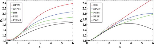
The ICFs of all GGA exchange functionals can be written as a function of either the reduced density gradient, x_σ, or a slightly different dimensionless variable, . Since the latter variable is well understood [49] and generally used to plot the ICFs of non-empirical GGA exchange functionals, Figure 2 plots the ICFs for a handful of popular GGA exchange functionals as a function of (the spin-unpolarised version of s_σ). A horizontal line at g_x = 1 represents the LDA exchange functional, and these ICFs represent corrections to the LDA. The plots are useful in explaining the behaviour of certain functionals for bonded interactions (i.e. the set of 124 atomisation energies). For example, it is evident that the PBE and PBEsol exchange ICFs differ such that PBEsol deviates less from the LDA than PBE does. Accordingly, this is reflected in the performance of PBEsol for the set of 124 atomisation energies, such that the MSE of PBEsol (-28.56 kcal/mol) is somewhere between the MSE of SPW92 (-58.11 kcal/mol) and the MSE of PBE (-12.17 kcal/mol). On the other hand, revPBE has an even stronger density gradient dependence than PBE, and as a result, its MSE is remarkably close to zero (0.74 kcal/mol).

Figure 2. Inhomogeneity correction factors (ICF) for a variety of GGA exchange functionals as a function of . The subfigure on the left contains exchange functionals with ICFs that are PBE-like, while the subfigure on the right contains exchange functionals with ICFs that differ substantially from the PBE form. The local density approximation is equivalent to a horizontal line at g_x = 1.

Two additional independent ingredients [50] that can be used to further improve the accuracy of density functionals are either the Laplacian of the density, ∇2ρσ, or the kinetic energy density, τσ = ∑nσi|∇φi, σ|2. Since these two ingredients, which capture second derivative information, are related [51] (Equation (11(11) )), only one or the other tends to appear in a given functional form (although there are exceptions [52]). The kinetic energy density is by far the more popular ingredient and has been used in many modern functionals to add flexibility to the functional form with respect to both constraint satisfaction and least-squares fitting. From a chemical perspective, the kinetic energy density can be useful for detecting electron delocalisation in molecules [53]. Functionals that depend on either of these ingredients define the third rung of Jacob's Ladder and are known as meta-generalised gradient approximations (meta-GGA or mGGA), (11)

While the reduced density gradient (x_σ or s_σ) is by far the most utilised dimensionless variable involving the density gradient, a variety of dimensionless variables involving the kinetic energy density have been proposed through the years [8,52,54–56]. The most popular [56], perhaps, is , or in spin-unpolarised form. This variable takes on values significantly smaller than one when the exchange hole is highly delocalised and is otherwise mostly on the order of one, except in two specific situations: exponential tails (t_σ ≈ 0) and stationary points of localised orbitals (t_σ ≈ ∞). As with x_σ, the range of t_σ is semi-infinite, [0,∞), and it is highly desirable to transform it to a finite domain: . A typical meta-GGA exchange functional can be represented by Equations (12(12) ) and (13(13) ), where the latter is a two-dimensional power series. Besides t_σ, a dimensionless variable [8] that is commonly used in meta-GGA functionals (particularly non-empirical ones) is . This variable is able to distinguish between different types of interactions, such as covalent (α = 0), metallic (α ≈ 1), and weak (α ≫ 1) bonds, (12) (13)

Popular non-empirical meta-GGA exchange-correlation functionals are almost exclusively from Perdew and co-workers, and include PKZB [54], TPSS [8], and revTPSS [57], as well as the newer MS0 [55], MS1 [14], MS2 [14], MVS [58], and SCAN [59] functionals. Additionally, the BLOC functional [60] by Della Sala and co-workers and the TM functional [61] by Tao and Mo represent two recent attempts at non-empirical meta-GGAs. Semi-empirical meta-GGA functionals are mainly due to the parameterisations provided by the Truhlar group, and include functionals such as M06-L [62], M11-L [63], MN12-L [64], and MN15-L [65]. Some earlier notable attempts at semi-empirical meta-GGAs include efforts by Scuseria (VSXC [66]) and Handy (τ-HCTH [67]), Goerigk and Grimme [68] (oTPSS), and a recent meta-GGA functional by Bligaard and co-workers, named mBEEF [69], is based on a Bayesian error estimation framework.

In general, meta-GGAs tend to outperform GGAs for atomisation energies and barrier heights, and a few can even incorporate some ‘medium-range’ dispersion (e.g. SCAN and M06-L bind the parallel-displaced benzene dimer, while both PBE and HCTH/147 predict entirely unbound potential energy curves (PEC)). However, meta-GGA functionals tend to be more sensitive to the integration grid relative to GGAs, and care must be taken when dealing with weakly interacting systems [70–72]. Referring again to Table 1, for the set of 124 atomisation energies, TPSS further reduces the MSE of PBE by more than a factor of 4, but worsens the performance of PBE for the hydrogen-bonded systems by converting the slight tendency of PBE to overbind to a greater tendency to underbind. For the dispersion-bound systems, TPSS is even more underbound than PBE.

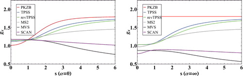
For a fixed value of , the ICFs of meta-GGA exchange functionals can be expressed as a function of s. Figure 3 plots the ICFs of several popular meta-GGA exchange functionals as a function of s for both α = 0 and α = ∞. Compared to the GGA exchange ICFs in Figure 2, it is evident that meta-GGA exchange functionals utilise density gradient information quite differently for covalent (α = 0) versus weak (α = ∞) bonds, whereas a GGA exchange functional like PBE has a fixed reduced density gradient behavior regardless of the value of α. Furthermore, comparing the exchange ICFs of three definitive meta-GGAs (PKZB, TPSS, and SCAN) at α = 0 indicates that significant changes have been made to non-empirical meta-GGA exchange functionals through the years.

Figure 3. Inhomogeneity correction factors (ICF) for a variety of meta-GGA exchange functionals as a function of . The subfigure on the left plots the α = 0 limit (covalent bonds), while the subfigure on the right plots the α = ∞ limit (weak bonds). The local density approximation is equivalent to a horizontal line at g_x = 1.

Despite the ‘systematic’ improvement offered by additional physical ingredients, there are three major limitations to the exchange-correlation functionals described above that cannot be remedied by the inclusion of local ingredients such as ρ, ∇ρ, and τ: (1) self-interaction error (SIE), (2) long-range dynamic correlation (dispersion), and (3) strong correlation.

The simplest way to demonstrate self-interaction[73] (electrons interacting with themselves) is to consider the HF description of the hydrogen atom. Since the hydrogen atom contains only one electron, the electron– electron interaction energy should be exactly zero. At the CBS limit, the HF energy for the hydrogen atom is -0.5 Hartrees (Eh), which comes from summing the kinetic (0.5 Eh), nuclear– electron attraction (-1.0 Eh), Coulomb (0.3125 Eh), and exchange (-0.3125 Eh) energy contributions. Thus, the classical and non-classical electron– electron contributions cancel each other exactly, making HF one-electron SIE-free. In KS-DFT, since the exact exchange term is replaced by the exchange-correlation functional, most functionals are not one-electron SIE-free[22] (i.e. J[ρ(r)] + E_xc[ρ(r)] ≠ 0 for the hydrogen atom).

A possible workaround for this issue is to replace the local exchange functional with the exact exchange functional (Hartree–Fock), while employing a local correlation functional that gives exactly zero correlation energy for any one-electron system (such as LYP). Early attempts at combining exact exchange with local correlation (e.g. HFLYP) were unsuccessful. For example, for the set of 124 atomisation energies, HFLYP is only able to reduce the MAD of HF by about a factor of 3, whereas a popular GGA functional such as BLYP (MAD of 6.51 kcal/mol) reduces the MAD of HF by almost a factor of 20. The idea of combining exact exchange and density functionals was therefore put on hold for a few years until the early 1990s, when Becke introduced the idea of mixing only a global fraction of exact exchange with the exchange-correlation functional[9,74] (an imperfect yet highly successful solution that defines Rung 4 of Jacob's Ladder). Most generally, these global hybrid (GH) functionals take the form given in Equation (14(14) ) and can be theoretically justified with the adiabatic connection formula[75–78]. A more empirical way to motivate global hybrid functionals is to consider the MSEs of HF and SPW92 for the set of 124 atomisation energies. While the former underestimates the atomisation energies with an MSE of 112.79 kcal/mol, the latter overestimates them with an MSE of -58.11 kcal/mol. Although an equal mixing of the two (c_x = 0.50) would still potentially lead to underbinding, a value of c_x = 0.34 will non-self-consistently lead to these MSEs summing to zero, (14)

The first global hybrid functional [9], B3PW91, was developed by Becke in 1993 by fitting three linear parameters to 56 atomisation energies. B3PW91 is a global hybrid GGA density functional that takes the form given in Equation (15(15) ), where c_x = 0.20, a_x = 0.72, and a_c = 0.81. For the set of 124 atomisation energies, B3PW91 further reduces the MAD of BLYP by a factor of nearly 2.5. Most global hybrid GGA density functionals have an exact exchange mixing parameter between 20% and 25%, including the most popular density functional, B3LYP (20%). B3LYP is nearly identical to B3PW91, with the only difference being that the PW92 and PW91 correlation functionals are replaced by the VWN1RPA [21] and LYP correlation functionals, respectively. Another popular three-parameter global hybrid GGA functional is B3P86, which is B3LYP with LYP replaced by P86. (15)

The most popular non-empirical global hybrid GGA is PBE0[79] (with 25% exact exchange), while the most popular semi-empirical global hybrid GGA (after B3LYP) is Becke's B97[10]. An alternative to PBE0 is revPBE0, which replaces the PBE exchange functional with revPBE exchange, while numerous attempts have been made to improve upon the semi-empirical B97 functional, including B97-1[36], B97-2[80], and B97-3[81]. For semi-empirical global hybrid GGAs, the value of c_x can change significantly depending on the systems in the training set. For example, the B97-K[82] and SOGGA11-X[83] density functionals have 42% and 40.15% exact exchange, respectively, because barrier heights were heavily emphasised in their construction. In general, the inclusion of exact exchange helps counter the overbinding of GGA functionals, at least for bonded interactions. For example, while PBE has an MSE of -12.17 kcal/mol for the set of 124 atomisation energies, PBE0 has an MSE of only 1.12 kcal/mol. While the difference between PBE and PBE0 for the dispersion-bound systems is entirely negligible, the addition of a fraction of exact exchange tends to ameliorate the tendency of PBE to slightly overbind the hydrogen-bonded systems, converting the -1.26 kcal/mol MSE of PBE to 0.20 kcal/mol. Consequently, the MAD of PBE (1.30 kcal/mol) is nearly halved by PBE0 (0.67 kcal/mol).

Naturally, the formula in Equation (15(15) ) can be extended to meta-GGAs to give global hybrid meta-GGA density functionals. From the non-empirical side, TPSSh[84], revTPSSh[85], and MS2h[14] have about 10% exact exchange, while the latest MVSh[58] and SCAN0[86] functionals have an uncharacteristically large value of c_x = 0.25. Since 2004, Truhlar has published at least 12 global hybrid meta-GGA density functionals, including MPW1B95[87], MPWB1K[87], PW6B95[88], PWB6K[88], M05[89], M05-2X[90], M06[91], M06-2X[91], M06-HF[92], M08-HX[93], M08-SO[93], and MN15[94]. The fraction of exact exchange across these functionals varies from 27% (M06) to 54% (M06-2X) to 100% (M06-HF). Other noteworthy global hybrid meta-GGAs include the semi-empirical BMK functional[82] with 42% exact exchange (intended for calculations of chemical kinetics), as well as τ-HCTHh[67] (15%) by Handy and co-workers.

While global hybrid functionals significantly improve upon their local counterparts for bonded interactions and kinetics, they only partially address the self-interaction issue. A more rigorous (yet still incomplete) approach to this problem is through range-separation[95,96], where the exact exchange contribution is split into a short-range component () and a long-range component (). The Coulomb operator of the short-range component is attenuated by the complementary error function, erfc(ωr₁₂), while the Coulomb operator of the long-range component is attenuated by the error function, erf(ωr₁₂). can be optionally scaled (c_{x, sr}) to give a non-zero fraction of short-range exact exchange, while the scaling coefficient (c_{x, lr}) of is usually set to one to ensure that the exchange functional is one-electron SIE-free in the long range. The corresponding local exchange functional should also be partitioned in the same way, with the short- and long-range components scaled by 1 − c_{x, sr} and 1 − c_{x, lr}, respectively. The functional form for a typical range-separated hybrid (RSH) functional is shown in Equation (16(16) ), (16)

Notable range-separated hybrid GGA functionals include the semi-empirical ωB97 and ωB97X functionals [13] from Chai and Head-Gordon, which have 0% and 15.77% short-range exact exchange, respectively, and tend to 100% exact exchange in the long-range (long-range corrected or LRC). The functionals have empirical values for ω, with the former having a value of ω = 0.4 and the latter a value of ω = 0.3. Less-empirical long-range corrected RSH GGA functionals include LC-ωPBE08 [97], LRC-ωPBE [98], and LRC-ωPBEh [98], which have ω values of 0.45, 0.3, and 0.2, respectively. The CAM-B3LYP RSH GGA functional[99] by Handy and co-workers is also very popular, particularly for excited state calculations. While it has 19% short-range exact exchange, its long-range coefficient is not 1, but rather 0.65, with an ω of 0.33. Finally, it is possible to entirely remove to form screened-exchange functionals, such as HSE-HJS [100,101] (HSE06 using the newer PBE exchange hole model from Reference [101]) and N12-SX [102], which are suitable for molecular as well as solid-state calculations. RSH meta-GGA functionals are the least common of the functional types mentioned thus far, with M11 [103] and MN12-SX [102] by Truhlar serving as two examples.

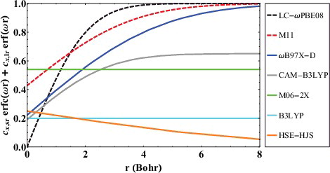
To help clarify the concept of range-separation, Figure 4 plots the exact exchange attenuators for various popular long-range corrected (ωB97X-D, CAM-B3LYP, LC-ωPBE, and M11) and screened-exchange (HSE-HJS) functionals, along with two global hybrid functionals (B3LYP and M06-2X) for comparison. As a point of reference, HF would be a horizontal line at y = 1. Beginning with the global hybrid functionals, since B3LYP has a fixed fraction of 20% exact exchange and M06-2X has a fixed fraction of 54% exact exchange, these functionals are simply characterised by horizontal lines at y = 0.2 and y = 0.54, respectively. The attenuators for the range-separated functionals are more interesting, and a functional like ωB97X-D has 22.2% short-range exact exchange and 100% long-range exact exchange, controlled by an ω of 0.2. The ω parameter controls the rate at which exact exchange turns on, and larger values of ω, as in LC-ωPBE08 (0.45), are less smooth, as they achieve full exact exchange much quicker. The HSE-HJS screened-exchange functional has 25% short-range exact exchange, and tends to 0% exact exchange in the long range, albeit very slowly, as its value of ω is only 0.11.

Figure 4. Exact exchange attenuation plots for various long-range corrected (ωB97X-D, CAM-B3LYP, LC-ωPBE, and M11), screened-exchange (HSE-HJS), and global hybrid (B3LYP and M06-2X) density functionals. As a point of reference, Hartree–Fock is equivalent to a horizontal line at y = 1.

The so-called ‘local hybrid’ functionals[104] represent yet another class that belongs on Rung 4 of Jacob's Ladder. Encompassing functionals such as B05 [105] and PSTS [106], they explicitly depend on the exchange energy density through a real-space-dependent local mixing function that can detect the character of the electron density and modulate between local and exact exchange, accordingly.

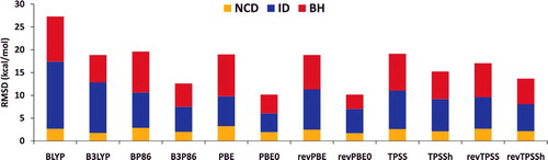
To further demonstrate the role of exact exchange in reducing SIE, Figure 5 shows root-mean-square deviations (RMSD) for a variety of local and hybrid functional pairs (e.g. BLYP and B3LYP) for classes of interactions that are sensitive to the inclusion of exact exchange. These include difficult non-covalent interactions (NCD) and isomerisation energies (ID) that are prone to electron delocalisation, as well as barrier heights (BH). Adding a fraction of exact exchange improves the performance of the local counterpart in all six cases, with the largest improvements belonging to PBE/PBE0 and revPBE/revPBE0, which have the highest fraction of exact exchange from the selected functionals (25%). On the other hand, the distinction between TPSS and TPSSh or revTPSS and revTPSSh is not very significant, due to the small fraction of 10% exact exchange that is utilised in these meta-GGAs. Nevertheless, it is clear that the inclusion of a fraction of exact exchange tends to significantly improve the performance of local functionals for these three categories.

Figure 5. Stacked root-mean-square deviations (RMSD) in kcal/mol for a set of six local/hybrid functional pairs (e.g. BLYP/B3LYP). NCD contains 91 non-covalent interactions that are sensitive to electron delocalisation, ID contains 155 isomerisation energies that are sensitive to electron delocalisation, while BH contains 206 barrier heights. Section 4.1 provides a more complete description of NCD, ID, and BH. These 452 data points are representative of cases where the addition of a fraction of exact exchange should improve the performance of a local functional. For example, the performance of PBE is improved by about a factor of 2 upon the introduction of 25% exact exchange (PBE0).

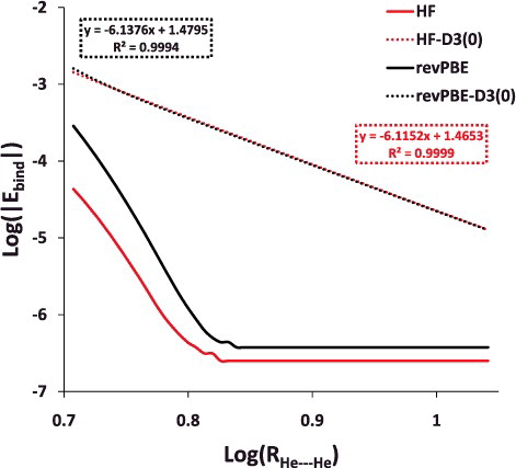
The second weakness of local and hybrid exchange-correlation functionals is their inability to properly account for long-range dynamic correlation. The most straightforward way to demonstrate this issue is to consider the PEC of a dispersion-bound system, such as the helium dimer. For this system, LSDA, GGA, meta-GGA, and hybrid functionals exhibit an exponential long-range decay, instead of the proper R⁻⁶ decay. This phenomenon is visually depicted in Figure 6. Fortunately, the past decade has seen a vast amount of work dedicated to improving the description of non-covalent interactions within KS-DFT [107]. The two most popular methods [108,109] are the DFT-D dispersion tails developed by Grimme and co-workers [110–113] and nonlocal correlation (NLC) functionals such as vdW-DF2 by Lundqvist and co-workers [114,115] and VV10 by Vydrov and Van Voorhis [116].

Figure 6. Log– log plot of the helium dimer potential energy curve with Hartree–Fock (HF) and revPBE, as well as their dispersion-corrected counterparts. The post-equilibrium portion of the curve (5.1 Å and larger) is displayed in order to demonstrate that the long range behaviour of the dispersion-corrected functionals is approximately R⁻⁶.

Grimme's DFT-D method is a damped, atom– atom empirical potential (Equation (17(17) )) that can be trained as an additive correction for any of the aforementioned functionals. Three generations of DFT-D tails have been developed by Grimme thus far: D1 [110], D2 [111], and D3 [112]. The D3 tail can be used either with the original damping function, D3(0), or the newer Becke-Johnson damping function [113], D3(BJ). Recently, Sherrill and co-workers [117] refit the D3(BJ) parameters for a set of eight density functionals, and these revised parameters are referred to as D3M(BJ). Additionally, Schwabe and co-workers [118] reformulated the D3(BJ) damping function to depend only on C₆ dispersion coefficients, defining the D3(CSO) damping function, (17)

While it is straightforward to train a dispersion correction onto an existing density functional (and many of the previously mentioned functionals have D2, D3(0), D3(BJ), D3M(BJ), and D3(CSO) parameterisations), simultaneously training a semi-empirical functional with a dispersion correction is more involved. The first successful attempt of the latter was Grimme's B97-D functional [111], a local GGA functional utilising the D2 tail. Recently, both the D3(0) and D3(BJ) tails have been refit to the existing local exchange-correlation functional of B97-D to give B97-D3(0) and B97-D3(BJ). Other examples include the ωB97X-D [119] (GGA) and ωM05-D [120] (meta-GGA) RSH functionals by Chai and co-workers, which use a slightly modified version of the D2 tail [119] (called CHG). Finally, the most recent functionals by Chai and co-workers, ωB97X-D3 [121] (GGA) and ωM06-D3 [121] (meta-GGA), are RSH functionals that utilise the D3(0) tail.

In general, dispersion corrections such as DFT-D should be used with functionals that tend to underbind non-covalent interactions (both strong and weak). However, fitting a dispersion correction to a functional like PBE is tricky, since PBE is already overbound for the binding energies of the 38 water clusters mentioned earlier. Consequently, PBE-D3(BJ) increases the MSE of PBE by a factor of almost 5 for these clusters (-5.86 vs. -1.26 kcal/mol). On the other hand, PBE-D3(BJ) drastically improves upon PBE for the 12 dispersion-bound systems. The same circumstances afflict the PBE0 functional, which has a remarkably small MSE of only 0.20 kcal/mol for the water clusters. However, the addition of the D3(BJ) dispersion tail leads to overbinding (-3.86 kcal/mol). Similar to PBE, however, PBE0 systematically underbinds the 12 alkane dimers, and the addition of the dispersion correction reduces the MSE from 3.37 to -0.02 kcal/mol.

While the DFT-D approach has been popular for at least a decade, NLC functionals such as VV10 have recently started to gain traction. The VV10 NLC functional takes the form given in Equation (18(18) ) and is far less empirical than the DFT-D approaches, as it only contains two fitted parameters. VV10 can either be trained onto an existing functional, or simultaneously trained with a semi-empirical functional. The VV10 NLC functional has been fit onto several of the aforementioned functionals [122], including BLYP, revPBE, HF, and B3LYP, as well as rPW86PBE and LC-ωPBE08. The two lattermost functionals were originally defined along with the VV10 NLC functional, and are known as VV10 and LC-VV10, respectively [116]. Recently, Mardirossian and Head-Gordon have utilised the VV10 NLC functional to parameterise three combinatorially optimised, semi-empirical density functionals (Section 3.3): ωB97X-V [18], an RSH GGA, B97M-V [19], a local meta-GGA, and ωB97M-V[20], an RSH meta-GGA. These functionals are remarkably accurate compared to other functionals that belong to the same rung, and are very lightly parameterised, with 12 linear parameters at most, (18)

Compared to the DFT-D approach, evaluating the VV10 energy and potential is more expensive, particularly for extended systems. Therefore, a modification [123] to the VV10 NLC kernel (called rVV10) was introduced by Sabatini and co-workers to allow for the efficient implementation of the NLC functional in periodic codes. The rVV10 NLC functional has recently been fit to the B97M-V parent functional, to give the B97M-rV functional [124]. Similarly, the SCAN meta-GGA functional has also been complemented [125] with rVV10, to give SCAN+rVV10. Upon publication of the rVV10 NLC functional, the parent functional of the VV10 density functional (rPW86 + PBE) was appended with the rVV10 NLC functional (with a modified nonlinear empirical parameter) to define the rVV10 density functional.

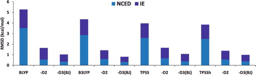
Figure 7 shows the effectiveness of dispersion corrections for non-covalent dimers (NCED) and isomerisation energies (IE). These datatypes differ from NCD and ID because the interactions in NCED and IE are not particularly sensitive to SIE. For the four sets of functionals considered (BLYP, B3LYP, TPSS, and TPSSh, along with their D2 and D3(BJ) counterparts), it is clear that the addition of even the most primitive dispersion correction offers a huge improvement over the uncorrected functional. Even more encouraging is the fact that the more recent D3(BJ) correction consistently improves upon the older D2 version.

Figure 7. Stacked root-mean-square deviations (RMSD) in kcal/mol for four density functionals and their D2 and D3(BJ) dispersion-corrected counterparts. The four parent functionals are BLYP (local GGA), B3LYP (hybrid GGA), TPSS (local meta-GGA), and TPSSh (hybrid meta-GGA). NCED contains 1744 non-covalent dimer interactions and IE contains 755 isomerisation energies. Section 4.1 provides a more complete description of NCED and IE. These 2499 data points are representative of cases where dispersion corrections should be very effective. Indeed, the performance of B3LYP is greatly improved by the addition of the older D2 dispersion tail, and even further refined when D2 is replaced by D3(BJ).

Finally, all of the aforementioned density functionals fail to some extent at describing multi-reference systems that are strongly correlated. The reason for this is simple: HF and KS-DFT are both single-determinant methods. In order to accurately describe a multi-reference system, it is necessary to include information from multiple determinants. Addressing the issue of strong correlation within KS-DFT is the least solved problem of the three mentioned thus far, and requires much further exploration[126–128]. However, local functionals and hybrids with a small fraction of exact exchange tend to perform acceptably for these types of systems. Additionally, it is possible to include multi-reference systems in the training set of a semi-empirical functional, such as MN15-L, at the cost of drastically worsening performance for single-reference interactions such as non-covalent interactions [129].

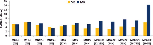
The effect of an increasing percentage of exact exchange on the performance of a functional for single-reference (SR) versus multi-reference (MR) bonded interactions such as atomisation energies, bond dissociation energies, and heavy-atom transfer reaction energies is demonstrated with the Minnesota family of functionals in Figure 8. For the local functionals, it is evident that the gap between the SR and MR RMSDs is rather small, and in some cases (such as MN15-L) the SR error can be larger than the MR error! However, as the fraction of exact exchange increases, the gap tends to widen, and the multi-reference RMSD is quite large by the time one gets to M06-HF, which has 100% exact exchange.

Figure 8. RMSD in kcal/mol for the 12 local and global hybrid Minnesota density functionals. SR contains 712 single-reference bonded interactions (124 atomisation energies, 505 heavy atom transfer reaction energies, and 83 bond dissociation energies), while MR contains 234 multi-reference bonded interactions (16 atomisation energies, 202 heavy atom transfer reaction energies, and 16 bond dissociation energies). The percentage of global exact exchange is displayed under the name of each functional. These 946 data points demonstrate the tradeoff between exact exchange and performance for single- and multi-reference interactions. For example, M06, with 27% exact exchange, performs equally well for SR and MR, while M06-2X, with 54% exact exchange, performs nearly 30% better than M06 for SR, but more than 30% worse than M06 for MR.

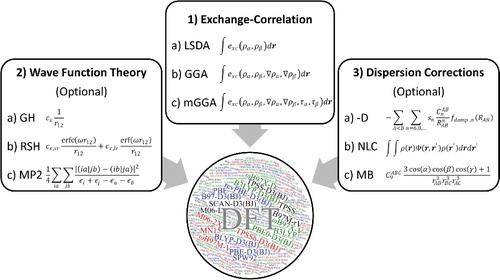
In order to conclude this practical introduction to DFT, it is helpful the summarise the different types of density functionals that can be constructed with the components discussed thus far. While Jacob's Ladder represents an accepted conceptualisation of the DFT hierarchy, an alternate view of the composition of density functionals is given in Figure 9. This visualisation is helpful, as most existing density functionals can be described by combining one (or more) component from each of the three primary categories: (1) exchange-correlation, (2) wave function theory, and (3) dispersion corrections. The first component, exchange-correlation, exactly coincides with the first three rungs of Jacob's Ladder (LSDA, GGA, or meta-GGA). The next component, wave function theory, is optional and refers to contributions such as exact exchange or perturbation theory. The last component, dispersion corrections, is also optional and refers to the aforementioned treatments developed for non-covalent interactions such as the DFT-D approach, NLC functionals, and other many-body corrections. To give an example of the utility of this figure, B3LYP-D3(BJ) corresponds to the combination of 1b+2a+3a, while PBE simply corresponds to 1b. A more complicated functional, such as the double hybrid B2PLYP-D3(BJ) functional [130,131], corresponds to 1b+2a+2c+3a (double hybrids [132], which depend on virtual orbitals, will not be discussed in this review).

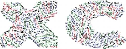
Figure 9. A graphical representation of elements that can be combined to define most existing density functionals. The circle contains the names of the 200 density functionals that are considered in this review, with the 20 featured functionals appearing in larger letters.

3. Semi-empirical density functionals

3.1. Development and survey

The idea of fitting density functional parameters to best reproduce a set of reference values (e.g. HF atomic exchange energies, CCSD(T)/CBS data, experimental data, etc.) is decades old. In the 1950s, before the formal foundations of DFT had been established, the Xα method[133] was proposed by John Slater as a simplification of HF. In fact, the Xα method is equivalent to performing a KS-DFT calculation with the exchange-correlation functional replaced by the exchange-only functional shown in Equation (19(19) ). With a value of α = 2/3, the Xα method is equivalent to the LSDA exchange functional in Equation (7(7) ). However, in order to accurately reproduce atomic exchange energies [134–136], the optimal value of α ranges from 0.7 (for heavier atoms such as krypton) to 0.8 (for lighter atoms such as helium). (19)

Until the early 1990s, fitting parameters to reproduce HF atomic exchange energies or accurate atomic correlation energies was perhaps the most commonly utilised approach. For example, this was done to obtain an empirical estimate for β in the Xαβ exchange functional [136], as well as to determine atom-specific values of α in the Xα method, as already mentioned. Furthermore, Becke's B86 and B88 exchange functionals had free nonlinear parameters that were fit to minimise errors for a set of atomic exchange energies. With the B3PW91 density functional (Equation (15(15) )), Becke switched gears and used least squares to fit three linear coefficients to minimise errors in the atomisation energies of the G2 test set [137]. This opened up the doors to the design of density functionals via least squares fitting to molecular properties instead of atomic properties.

Becke expanded upon his B3PW91 idea with the B97 density functional (Equation (20(20) )), a global hybrid GGA with three individual power series enhancing three separate UEG energy densities: exchange, same-spin correlation, and opposite-spin correlation. The two correlation components were acquired by employing a useful trick introduced by Stoll and co-workers [138]. In Equation (20(20) ), the latter three terms are very similar to Equation (8(8) ), besides the change in the associated energy density (i.e. vs. vs. ) and ICF (i.e. vs. vs. ). Becke expanded the three power series uniformly from zeroth order up to eight order, and the goodness of fit to the training set indicated that the optimal truncation was at second order, resulting in a functional with 10 parameters (c_x and three power series contributing three linear parameters each), (20)

The influence of the B97 density functional on the development of semi-empirical density functionals has been very significant. Ever since the publication of B97, a vast number of functionals have been parameterised in a similar fashion, and a selection of semi-empirical density functionals based on the B97 concept is listed below (dispersion-corrected functionals are underlined):

• GGA functionals

  • Local: HCTH/93, HCTH/120, HCTH/147, HCTH/407, B97-D, SOGGA11 [36–38,111,139]

  • Global hybrid: B97-1, B97-2, B97-K, B97-3, SOGGA11-X [36,80–83]

  • Range-separated hybrid: ωB97, ωB97X, ωB97X-D, ωB97X-D3, ωB97X-V[13,18,119,121]

• NGA functionals

  • Local: N12, GAM [39,40]

  • Range-separated hybrid: N12-SX [102]

• meta-GGA functionals

  • Local: τ-HCTH, M06-L, M11-L, B97M-V[19,62,63,67]

  • Global hybrid: τ-HCTHh, BMK, M05, M05-2X, M06, M06-2X, M06-HF, M08-HX, M08-SO [67,82,89–93]

  • Range-separated hybrid: M11, ωM05-D, ωM06-D3, ωB97M-V [20,103,120,121]

• meta-NGA functionals

  • Local: MN12-L, MN15-L[64,65]

  • Global hybrid: MN15[94]

  • Range-separated hybrid: MN12-SX[102]

Most of the functionals listed above use the ingredients contained in Figure 10, or slight variants thereof. The only exceptions are the so-called nonseparable gradient approximation (NGA) and meta-NGA functionals, which use an additional variable that only depends on the density: . The distinction between GGA and NGA functionals or meta-GGA and meta-NGA functionals is not made in this review, because NGA functionals are practically GGAs (depend on the density and its gradient), and meta-NGA functionals are practically meta-GGAs (depend on the density, its gradient, and the kinetic energy density). It is noteworthy that some of the resulting NGA and meta-NGA functionals have been demonstrated to be overfitted and ill-behaved[16,129,140].

Figure 10. Ingredients that are conventionally used in the functional forms of semi-empirical density functionals. The primary GGA variable is the density gradient, ∇ρ, while the primary meta-GGA variable is the kinetic energy density, τ.

The general form for the power series utilised in GGA functionals is given in Equation (9(9) ). Conventionally, the value of N (the truncation order for the summation) has either been chosen a priori or determined based on a ‘goodness-of-fit’ to the training set (like with B97). Smaller values of N can yield smoother and perhaps more transferable ICFs, while larger values necessarily provide better fits to training data, whose transferability must be subsequently assessed on an independent test set. While B97 is an example of a functional that utilises N = 2, more recent semi-empirical functionals have utilised N = 4 (B97-3 and ωB97X) or even N = 5 (SOGGA11-X).

In contrast to the one-dimensional power series that characterises a GGA density functional, the most general power series that can accommodate a meta-GGA density functional using the two variables in the last row of Figure 10 is the power series given in Equation (13(13) ). For meta-GGA functionals, the values of N and N′ must be determined cautiously, as selecting values that are too large might result in ill-behaved functionals. For example, while a GGA functional with N = 4 has five free parameters per power series, a meta-GGA with N = N′ = 4 will have 25.

3.2. Counting semi-empirical parameters

With semi-empirical density functionals, a measure that is commonly reported upon publication is the total number of parameters. Existing functionals based on the B97 concept have anywhere between 5 and 75 parameters. However, counting the number of parameters is often a confusing and unclear task. As an example, upon publication of the M11 density functional in Reference [103], the authors indicated that the functional had 38 parameters. A year later, upon the publication of the M11-L density functional in Reference [63], the same authors indicated that M11 had 40 parameters. Across these two papers, the number of parameters for several functionals also changed. M08-HX changed from having 47 parameters to 44, while ωB97X and ωB97X-D changed from having 33 parameters, to 14 and 15, respectively. The reason for these discrepancies originates in the fact that semi-empirical density functionals have a variety of different parameter classes. For example, there are parameters that come from the local DFT components (e.g. the power series), there are parameters that come from the components that handle dispersion (e.g. s₆ from DFT-D), and there are parameters that come from wave function theory (e.g. c_x from exact exchange). Furthermore, within these three categories, the parameters can be linear or nonlinear. For example, with the power series, while the coefficients themselves are linear parameters, the parameter γ in u_σ is nonlinear. The same applies to dispersion tails (s₆ is linear while s_{r, 6} is nonlinear in D3(0)) and exact exchange (c_x is a linear parameter while the range-separation parameter, ω, is nonlinear).

All of these aforementioned parameters can be determined in one of three ways: (1) fitted during development, (2) borrowed from an existing functional, or (3) preset based on sound arguments. Fitted parameters are simply those determined by minimising the error in a training set. Borrowed parameters are quite common but are typically of the nonlinear variety, since performing a nonlinear optimisation is far more costly than using linear least-squares, and multiple local minima may be encountered. As an example, the three γ parameters used for the exchange, same-spin correlation, and opposite-spin correlation versions of u_σ were optimised during the development of the B86 exchange functional and the B97 density functional, and have been inserted into numerous functionals including B97-1, B97-2, B97-K, B97-D, the entire HCTH-family of functionals, the entire ωB97-family of functionals, and BMK, to name a few. Preset parameters are less common, but many popular functionals have made use of this procedure. For example, with B97-D, Grimme set the value of s₆ to 1.25 in order to restrict the local components to a shorter length scale. Another example of a preset parameter value is the fraction of exact exchange for M06-2X, which is double that of M06. An important factor that comes into play when counting parameters is the number of constraints used during the least-squares procedure. Some functionals, like the original B97, employ no constraints. The most common constraint is exactness for the UEG, and this is upheld by many functionals, including ωB97, ωB97X, and the 2005–2011 Minnesota functionals. The M11-L functional uses a total of 11 constraints, including the correct second-order term in the density gradient expansion, as well as constraints on the extremes of the kinetic energy dependent term for exchange.

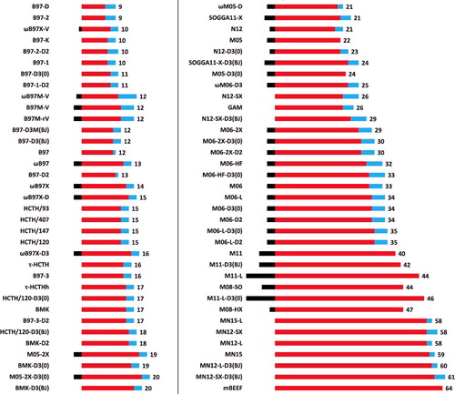
Of the 200 functionals considered in this work, 70 of them are based on the B97 concept. In the Supplemental Data, parameter details are given for these 70 functionals, with breakdowns that take into consideration the component (local DFT, dispersion, or wave function theory), the type (linear or nonlinear), and the origin (fitted, borrowed, or preset). However, a refined version is presented in Figure 11. The red bars indicate the number of fitted parameters, while the blue bars count the total number of borrowed or preset parameters. Furthermore, the black bars that begin at zero and proceed left represent the number of constraints which subtract from the total number of fitted parameters. The values off to the right indicate the total number of fitted parameters (red) minus the number of constraints (black), thus excluding borrowed or preset parameters. Based on this particular method of counting parameters, M11 has 40 parameters, while the functional with the most parameters is mBEEF, at 64. Most of the functionals on the right side of the figure (besides mBEEF) come from the Truhlar group, with the exception of ωM05-D and ωM06-D3, which were developed by Chai and co-workers by modifying the functional forms of M05-2X and M06-2X, respectively. The functionals on the left side have relatively fewer parameters, ranging from 9 (B97-D) to 20 (BMK-D3(BJ)). At the other extreme, largely as a consequence of avoiding overfitting, the combinatorially optimised functionals (Section 3.3) by Mardirossian and Head-Gordon have very few parameters, with 12 at most. It is interesting to point out that every single functional has at least one borrowed or preset parameter, since even the original B97 functional borrowed a nonlinear parameter from the B86 exchange functional.

Figure 11. (Colour online) A visual depiction of parameter counting in semi-empirical density functionals. The middle (red) bars indicate the number of fitted parameters, while the right (blue) bars count the total number of borrowed or preset parameters. Furthermore, the left (black) bars that begin at zero and proceed left represent the number of constraints which subtract from the total number of fitted parameters. The values off to the right indicate the total number of fitted parameters (middle, red) minus the number of constraints (left, black), thus excluding borrowed or preset parameters. For example, ωB97X has 17 fitted parameters, 3 borrowed or preset parameters, and utilises 3 constraints, for a total of 14 parameters.

3.3. Combinatorial functional design

The design challenge in semi-empirical density functionals is to make an appropriate truncation of a chosen functional form (i.e. select maximum values for N and N′) that maximises predictive power, while avoiding the potential overfitting problem. In Becke's original work, this issue was addressed by choosing the largest value of N which yielded expansion coefficients associated with smooth ICFs. However, such a procedure is somewhat qualitative and does not necessarily ensure the highest possible predictive power, as evidenced by the fact that other B97-based functionals have made truncations at slightly higher N values and still worked effectively. Recent work on this problem by the present authors [17–20] takes a much more exhaustive approach. In order to define the space of possible functionals, values for N and N′ are chosen, followed by an attempt to consider all possible combinations of the coefficients via best-subset selection. Using this ‘combinatorial’ approach leads to a total of fits ranging from 1 through T parameters, instead of just a handful (i.e. a total of nine fits were explored before selecting the functional form for the B97 density functional).

In the case of a B97-like meta-GGA with three components described by power series resembling Equation (13(13) ), the total number of available parameters, T = 3(N′ + 1)(N + 1), is quite large. However, with a large number of candidate fits, the transferability of the fits can be assessed on an independent test set, allowing them to be ranked based on both their training set and test set performance. Furthermore, fits can be discarded based on undesirable physical characteristics or other relevant criteria. Setting N′, the meta-GGA maximum truncation order, to 8, and N, the GGA maximum truncation order, to 4, as was done initially with the B97M-V and ωB97M-V functionals, brings the total number of possible combinations to an astounding 2¹³⁵ − 1 ≈ 10⁴¹, a ‘functional genome’ whose rank is approaching the square of Avogadro's number. Besides the linear parameters arising from the power series, the value of T can be incremented by including an optimisable fraction of global, short-range, or long-range exact exchange. Additionally, linear parameters from dispersion corrections (e.g. DFT-D, VV10, etc.) or wave function theory (e.g. MP2, OS-MP2, etc.) can further increase the complexity of the combinatorial search by slightly increasing the value of T.

When the value of T is small and performing the entire set of Q fits is feasible, it is possible to explore the entire functional space without resorting to any approximations. Given a GGA functional with three components (exchange, same-spin correlation, and opposite-spin correlation), a generous choice of N = 5 only results in 2¹⁸ − 1 = 262, 143 possible fits, a number that is easily manageable. Exploring functional spaces with T as large as 35 or even 40 is possible, but becomes unfeasible for larger values of T. With T = 135, Q is impossibly large, and the binomial coefficients themselves begin to increase in magnitude very quickly. For example, there are possible 1-parameter fits, possible 2-parameter fits, possible 3-parameter fits, possible 4-parameter fits, possible 5-parameter fits, possible 6-parameter fits, and so on.

The point at which a certain binomial coefficient becomes computationally unfeasible depends to a certain extent on the available computational resources. During the development of B97M-V and ωB97M-V, the present authors found that around 10⁹ fits could be performed on a 64-core node in a day, given the size of the training and test sets. Consequently, performing fits takes three days on a 64-core node, exploring all fits with just one more parameter (7) will take around two months on a 64-core node, while exploring all 8-parameter fits will take several years. It is certainly possible to split the task over hundreds of nodes, but even with 1000 nodes, exploring all 10-parameter fits would take half a year. Therefore, at a certain point, the exploration of fits with more parameters becomes unfeasible, and further approximations are necessary to conduct a more exhaustive search.

One option is to employ a method conceptually similar to a statistical tool called forward-stepwise selection. Once the binomial coefficients become too large to be computationally feasible (e.g. at ), it is necessary to find a way to explore 7-parameter and 8-parameter fits and so on. Therefore, the best 6-parameter fits (with respect to both training and test set performance) from the run can be analysed, and the most significant parameter can be identified and compulsorily-selected (or frozen, not to be confused with fixing its value) in the next set of fits. Freezing F commonly occurring parameters, allows for the exploration of (T − F)Ck (k + F)-parameter fits. For example, if the results from indicate that c_{x, 01} is the most important parameter, a possible next step would be to freeze c_{x, 01} (again, not its value but simply its inclusion in all successive fits) and explore the 7-parameter fits that mandatorily contain c_{x, 01}.

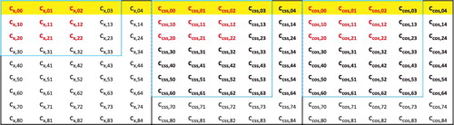
However, this approach should be used with care, because within the meta-GGA parameter space, it is likely that fits with fewer parameters will prefer GGA-only variables. For example, it is entirely possible for the best 6-parameter fit from a run to be a GGA functional. Therefore, it is important to make sure that the freezing is initiated at a large enough value of k, such that there is no heavy bias toward the GGA-only variables (i.e. c_{x, 01}, c_{x, 02}, etc.). In order to be able to sample fits with more than six parameters without freezing, the value of T must be reduced, and this can be done by exploring different truncations of the parameter space. For example, during the development of ωB97M-V, it became apparent that exchange variables past quadratic order were not appearing in the best fits. Therefore, truncating the exchange space of 45 variables to just quadratic terms (9 variables) helped lower the complexity of the problem by decreasing T from 135 to 99. The same concept can be applied to the same-spin and opposite-spin correlation variable spaces. Figure 12 shows various truncations of the parameter space, with the bold coefficients representing the space from which ωB97M-V was selected.

Figure 12. (Colour online) A visualisation of an (eighth-order meta-GGA) x (fourth-order GGA) functional space, which can be constructed by the two-dimensional power series in Equation (13(13) ) with N′= 2N= 8. The three separate blocks (from left to right) contain exchange, same-spin correlation, and opposite-spin correlation coefficients, respectively. Different truncations of the parameter space are shown, with the red coefficients representing up to quadratic fits in all three components, the highlighted coefficients representing the GGA-only subspace, and the blue boxes representing third order in exchange and sixth/third order in the meta-GGA/GGA dimension in both correlation components.

Thus far, only the selection of the functional form has been discussed. However, if the combinatorial approach is not used, this process is rather simple and involves simply selecting the coefficients that will be determined by a least-squares fit. Naturally, the coefficients themselves will have to be self-consistently optimised. There are several other factors besides the functional form itself that must be considered in the course of semi-empirical density functional development. For example, in order to generate the data that is needed to carry out these least-squares fits, it is necessary to choose an initial guess (i.e. pick the starting set of orbitals). A better guess will more closely resemble the composition of the final intended functional. For a local GGA or meta-GGA functional, the simplest and most general initial guess is the LSDA. However, for a hybrid functional, starting with an LSDA guess might not be the best choice, as the exclusion of exact exchange might greatly affect the electron density and consequently the contributions from the local variables, causing the predicted residuals to differ drastically from the final results upon self-consistent optimisation of the parameters. Therefore, for a hybrid functional, it might be helpful to start with a standard fraction of exact exchange (e.g. 20%). Another common consideration is constraints during fitting. The most obvious ones are the UEG constraints, and these can be upheld by ensuring that c_{x, 00} = c_{css, 00} = c_{cos, 00} = 1 for a local functional, or c_{x, 00} + c_x = c_{css, 00} = c_{cos, 00} = 1 for a global hybrid. More complicated constraints can be used on the functional form, and a functional[93] like M08-SO respects the gradient expansion to second order for both exchange and correlation. Finally, the selection of the weights is an open-ended issue and there is no consensus on an optimal scheme, at least in the context of density functional development. For more information on the fitting procedure, the reader is referred to Section VI of Reference [20].

4. Computational details

4.1. Database for assessment

The database used to assess the performance of the density functionals in this review contains 84 data-sets (Table 2) and 4986 data points, and is named the Main-Group Chemistry DataBase (MGCDB84). These data-sets have been compiled from the benchmarking activities of numerous groups, including Hobza, Sherrill, Truhlar, Herbert, Grimme, Karton, and Martin. The reference data are typically estimated to be at least 10 times more accurate than the very best available density functionals, so that robust and meaningful conclusions can be drawn. Of the 84 data-sets, 82 are categorised into eight datatypes: NCED, NCEC, NCD, IE, ID, TCE, TCD, and BH. The two data-sets that are excluded from the datatype categorisation are AE18 (absolute atomic energies) and RG10 (rare-gas dimer PECs). The first three datatypes (NCED, NCEC, and NCD) pertain to non-covalent interactions (NC), the next two datatypes (IE and ID) pertain to isomerisation energies (I), the next two datatypes (TCE and TCD) pertain to thermochemistry (TC), and the last datatype pertains to barrier heights (BH). Since the eight datatypes will be heavily referenced in the rest of this review, it is important to establish a solid understanding of the types of interactions that belong to each category, as well as the origin of the abbreviations. The datatype abbreviations begin with letters corresponding to one of the four main categories: NC, I, TC, or BH. Appending one of the four main categories with the letter ‘E’ indicates that the interactions within are considered to be ‘easy’ cases (not very sensitive to self-interaction error or strong correlation), while the letter ‘D’ indicates that the interactions are considered to be ‘difficult’. Finally, for the non-covalent interactions only, the presence of a fourth letter, either ‘D’ or ‘C’, indicates the presence of dimers or clusters, respectively.

Table 2. Summary of the 84 data-sets that comprise MGCDB84. The datatypes are explained in Section 4.1. The fifth column contains the root-mean-squares of the data-set reaction energies. PEC stands for potential energy curve, SR stands for single-reference, MR stands for multi-reference, Bz stands for benzene, Me stands for methane, and Py stands for pyridine.

Name	Datatype	#	Description	ΔE (kcal/mol)	Ref.
A24	NCED	24	Binding energies of small non-covalent complexes	2.65	154
DS14	NCED	14	Binding energies of complexes containing divalent sulfur	3.70	155
HB15	NCED	15	Binding energies of hydrogen-bonded dimers featuring ionic groups common in biomolecules	19.91	156
HSG	NCED	21	Binding energies of small ligands interacting with protein receptors	6.63	157,158
NBC10	NCED	184	PECs for BzBz (5), BzMe (1), MeMe (1), BzH2S (1), and PyPy (2)	1.91	158–161
S22	NCED	22	Binding energies of hydrogen-bonded and dispersion-bound non-covalent complexes	9.65	141,158
X40	NCED	31	Binding energies of non-covalent interactions involving halogenated molecules	5.26	162
A21x12	NCED	252	PECs for the 21 equilibrium complexes from A24	1.43	163
BzDC215	NCED	215	PECs for benzene interacting with two rare-gas atoms and eight first- and second-row hydrides	1.81	164
HW30	NCED	30	Binding energies of hydrocarbon-water dimers	2.34	165
NC15	NCED	15	Binding energies of very small non-covalent complexes	0.95	166
S66	NCED	66	Binding energies of non-covalent interactions found in organic molecules and biomolecules	6.88	142,167
S66x8	NCED	528	PECs for the 66 complexes from S66	5.57	142
3B-69-DIM	NCED	207	Binding energies of all relevant pairs of monomers from 3B-69-TRIM	5.87	168
AlkBind12	NCED	12	Binding energies of saturated and unsaturated hydrocarbon dimers	3.14	47
CO2Nitrogen16	NCED	16	Binding energies of CO2 to molecular models of pyridinic N-doped graphene	3.84	169
HB49	NCED	49	Binding energies of small- and medium-sized hydrogen-bonded systems	14.12	170–172
Ionic43	NCED	43	Binding energies of anion-neutral, cation-neutral, and anion-cation dimers	69.94	173
H2O6Bind8	NCEC	8	Binding energies of isomers of (H2O)6	46.96	143,174
HW6Cl	NCEC	6	Binding energies of Cl^−(H2O)n (n = 1 − 6)	57.71	143,174
HW6F	NCEC	6	Binding energies of F^−(H2O)n (n = 1 − 6)	81.42	143,174
FmH2O10	NCEC	10	Binding energies of isomers of F^−(H2O)10	168.50	143,174
Shields38	NCEC	38	Binding energies of (H2O)n (n = 2 − 10)	51.54	48
SW49Bind345	NCEC	31	Binding energies of isomers of SO4^2 −(H2O)n (n = 3 − 5)	28.83	175
SW49Bind6	NCEC	18	Binding energies of isomers of SO4^2 −(H2O)6	62.11	175
WATER27	NCEC	23	Binding energies of neutral and charged water clusters	67.48	68,176
3B-69-TRIM	NCEC	69	Binding energies of trimers, with three different orientations of 23 distinct molecular crystals	14.36	168
CE20	NCEC	20	Binding energies of water, ammonia, and hydrogen fluoride clusters	30.21	177,178
H2O20Bind10	NCEC	10	Binding energies of isomers of (H2O)20 (low-energy structures)	198.16	143
H2O20Bind4	NCEC	4	Binding energies of isomers of (H2O)20 (dod, fc, fs, and es)	206.12	68,176,179,180
TA13	NCD	13	Binding energies of dimers involving radicals	22.00	144
XB18	NCD	8	Binding energies of small halogen-bonded dimers	5.23	181
Bauza30	NCD	30	Binding energies of halogen-, chalcogen-, and pnicogen-bonded dimers	23.65	182,183
CT20	NCD	20	Binding energies of charge-transfer complexes	1.07	184
XB51	NCD	20	Binding energies of large halogen-bonded dimers	6.06	181
AlkIsomer11	IE	11	Isomerisation energies of n = 4 − 8 alkanes	1.81	185
Butanediol65	IE	65	Isomerisation energies of butane-1,4-diol	2.89	186
ACONF	IE	15	Isomerisation energies of alkane conformers	2.23	68,187
CYCONF	IE	11	Isomerisation energies of cysteine conformers	2.00	68,188
Pentane14	IE	14	Isomerisation energies of stationary points on the n-pentane torsional surface	6.53	189
SW49Rel345	IE	31	Isomerisation energies of SO4^2 −(H2O)n (n = 3 − 5)	1.47	175
SW49Rel6	IE	18	Isomerisation energies of SO4^2 −(H2O)6	1.22	175
H2O16Rel5	IE	5	Isomerisation energies of (H2O)16 (boat and fused cube structures)	0.40	146
H2O20Rel10	IE	10	Isomerisation energies of (H2O)20 (low-energy structures)	2.62	143
H2O20Rel4	IE	4	Isomerisation energies of (H2O)20 (dod, fc, fs, and es)	5.68	68,176,179,180
Melatonin52	IE	52	Isomerisation energies of melatonin	5.54	190
YMPJ519	IE	519	Isomerisation energies of the proteinogenic amino acids	8.33	145
EIE22	ID	22	Isomerisation energies of enecarbonyls	4.97	191
Styrene45	ID	45	Isomerisation energies of C8H8	68.69	147
DIE60	ID	60	Isomerisation energies of reactions involving double-bond migration in conjugated dienes	5.06	192
ISOMERIZATION20	ID	20	Isomerisation energies	44.05	46
C20C24	ID	8	Isomerisation energies of the ground state structures of C20 and C24	36.12	193
AlkAtom19	TCE	19	n = 1 − 8 alkane atomisation energies	1829.31	185
BDE99nonMR	TCE	83	Bond dissociation energies (SR)	114.98	46
G21EA	TCE	25	Adiabatic electron affinities of atoms and small molecules	40.86	68,137
G21IP	TCE	36	Adiabatic ionisation potentials of atoms and small molecules	265.35	68,137
TAE140nonMR	TCE	124	Total atomisation energies (SR)	381.05	46

Table 2. Continued

Name	Datatype	#	Description	ΔE (kcal/mol)	Ref.
AlkIsod14	TCE	14	n = 3 − 8 alkane isodesmic reaction energies	10.35	185
BH76RC	TCE	30	Reaction energies from HTBH38 and NHTBH38	30.44	68,150,151
EA13	TCE	13	Adiabatic electron affinities	42.51	194
HAT707nonMR	TCE	505	Heavy-atom transfer energies (SR)	74.79	46
IP13	TCE	13	Adiabatic ionisation potentials	256.24	194
NBPRC	TCE	12	Reactions involving NH3/BH3 and PH3/BH3	30.52	68,195,196
SN13	TCE	13	Nucleophilic substitution energies	25.67	46
BSR36	TCE	36	Hydrocarbon bond separation reaction energies	20.06	148,196
HNBrBDE18	TCE	18	Homolytic N–Br bond dissociation energies	56.95	197
WCPT6	TCE	6	Tautomerisation energies for water-catalysed proton-transfer reactions	7.53	198
BDE99MR	TCD	16	Bond dissociation energies (MR)	54.51	46]
HAT707MR	TCD	202	Heavy-atom transfer energies (MR)	83.41	46
TAE140MR	TCD	16	Total atomisation energies (MR)	147.20	46
PlatonicHD6	TCD	6	Homodesmotic reactions involving platonic hydrocarbon cages, CnHn (n = 4, 6, 8, 10, 12, 20)	136.71	149
PlatonicID6	TCD	6	Isodesmic reactions involving platonic hydrocarbon cages, CnHn (n = 4, 6, 8, 10, 12, 20)	96.19	149
PlatonicIG6	TCD	6	Isogyric reactions involving platonic hydrocarbon cages, CnHn (n = 4, 6, 8, 10, 12, 20)	356.33	149
PlatonicTAE6	TCD	6	Total atomisation energies of platonic hydrocarbon cages, CnHn (n = 4, 6, 8, 10, 12, 20)	2539.27	149
BHPERI26	BH	26	Barrier heights of pericyclic reactions	23.15	68,199
CRBH20	BH	20	Barrier heights for cycloreversion of heterocyclic rings	46.40	200
DBH24	BH	24	Diverse barrier heights	28.34	201,202
CR20	BH	20	Cycloreversion reaction energies	22.31	203
HTBH38	BH	38	Hydrogen transfer barrier heights	16.05	151
NHTBH38	BH	38	Non-hydrogen transfer barrier heights	33.48	150
PX13	BH	13	Barrier heights for proton exchange in water, ammonia, and hydrogen fluoride clusters	28.83	177,178
WCPT27	BH	27	Barrier heights of water-catalysed proton-transfer reactions	38.73	198
AE18	–	18	Absolute atomic energies of hydrogen through argon	148,739.00	204
RG10	–	569	PECs for the 10 rare-gas dimers involving helium through krypton	1.21	152

The first datatype, NCED (non-covalent ‘easy’ dimers), is comprised of 18 data-sets and 1744 data points, and contains conventional, closed-shell, non-covalent dimer binding energies. Typical systems include the methane dimer, various orientations of the benzene dimer, the water dimer, almost 100 PECs of hydrogen-bonded, dispersion-bound, and mixed systems, as well as a handful of charged interactions. Popular data-sets that belong to NCED include S22 [141] and S66 [142] by Hobza and co-workers.

The NCEC datatype (non-covalent ‘easy’ clusters) is comprised of 12 data-sets and 243 data points, and contains binding energies of molecular clusters, including water clusters from trimers to 20-mers, ammonia clusters, hydrogen fluoride clusters, sulphate– water clusters, and solvated anions (both fluoride and chloride surrounded by multiple waters). The H2O6Bind8 data-set [143] belongs to the NCEC datatype and contains the binding energies of eight isomers of the water hexamer.

The final datatype that is classified under the NC umbrella is NCD (non-covalent ‘difficult’). The NCD datatype is comprised of 5 data-sets and 91 data points, and contains binding energies of halogen-bonded systems, interactions involving radicals, as well as charge-transfer complexes. A high fraction of exact exchange is essential for describing the types of systems in NCD. A sample data-set from NCD is TA13, which is extracted from a benchmark study on radical-solvent binary complexes [144]; mostly cases that are affected by self-interaction/delocalisation error.

Moving on to the isomerisation energies, IE (isomerisation energies ‘easy’) is comprised of 12 data-sets and 755 data points, and contains the relative energies of various alkanes, organic molecules, sulphate– water clusters, amino acids, and large water clusters. A representative from IE is the colossal YMPJ519 data-set [145] that contains 519 isomerisation energies involving the proteinogenic amino acids. Another interesting example is H2O16Rel5, which consists of the relative energies of the five lowest-energy water 16-mer structures [146].

The ID datatype (isomerisation energies ‘difficult’) is comprised of 5 data-sets and 155 data points, and contains isomerisation energies of enecarbonyls, conjugated dienes, and fullerenes. A fraction of exact exchange is helpful for describing the types of systems in ID. An interesting data-set from this datatype is Styrene45, which contains 45 isomers of C₈H₈, including highly strained fused rings and long cumulenic chains [147].

Moving on to the bonded interactions, TCE (thermochemistry ‘easy’) is comprised of 15 data-sets and 947 data points, and covers (single-reference) atomisation energies, bond dissociation energies, electron affinities, ionisation potentials, isodesmic reactions, reaction energies, heavy-atom transfer energies, and nucleophilic substitution energies. The large and useful W4-11 database [46] by Jan Martin and co-workers is the backbone of the TCE datatype, and another interesting data-set is BSR36, which contains 36 hydrocarbon bond separation reaction energies [148].

The TCD datatype (thermochemistry ‘difficult’) is comprised of 7 data-sets and 258 data points, and is mostly composed of the atomisation energies, bond dissociation energies, and heavy-atom transfer energies from W4-11 that are notoriously multi-reference in nature. However, 24 of the interactions involve platonic hydrocarbon cages [149] and are difficult cases for most density functionals. For the 234 multi-reference systems, however, local functionals and hybrids with a small fraction of exact exchange tend to perform best.

Finally, the BH datatype (barrier heights) is comprised of 8 data-sets and 206 data points, and contains pericyclic reactions, cycloreversion reactions, proton exchange reactions, as well as hydrogen transfer and non-hydrogen transfer barrier heights. The popular HTBH38 and NHTBH38 data-sets [150,151] by Truhlar and co-workers are found in BH, along with recent benchmark sets by Amir Karton and co-workers. As with the NCD and ID categories, a large fraction of exact exchange is helpful for an accurate description of barrier heights.

In addition to the eight datatypes discussed thus far, several of the data-sets within the NCED category (BzDC215, NBC10, and S66x8) contain potential energies curves that can be used to assess the accuracy of density functionals for predicting equilibrium properties of dimers (both equilibrium bond lengths (EBL) and equilibrium binding energies (EBE)). Furthermore, the RG10 data-set[152] contains all 10 PECs that can be constructed between the rare-gas dimers ranging from helium to krypton. In total, these four data-sets contain 96 PECs, with BzDC215, NBC10, and RG10 each having 10, and S66x8 having 66. Unfortunately, even with the use of a very fine grid, some of the resulting PECs are too oscillatory to be accurately interpolated [70–72], primarily for the Minnesota density functionals and functionals utilising a B95-like correlation component [153]. Consequently, the benzene– neon dimer and the benzene– argon dimer PECs from BzDC215 were removed, the sandwich benzene dimer, the methane dimer, and the sandwich (S2) pyridine dimer PECs from NBC10 were removed, and the helium dimer PEC from RG10 was removed, leaving a total of 90 PECs (9 rare-gas dimer PECs and 81 non-rare-gas dimer PECs). These 90 PECs will also be used to assess the performance of density functionals in the upcoming sections.

It should be noted, that a portion of this database was used to train the parameters of ωB97X-V, B97M-V, and ωB97M-V. For ωB97X-V and B97M-V, about 20% of this database served as the training set, while for ωB97M-V, the training set represented about 17.5% of this database. Furthermore, parts of this database were used to test millions of potential functional forms in order to select the most transferable fit. For ωB97X-V and B97M-V, an additional 20% of this database represented the test set, while for ωB97M-V, an additional 50% was used for testing purposes. Due to their design principles, these functionals contain such few fitted parameters (12 at most), that there is generally little difference between the training and test results.

4.2. Scope of computations

Although the sheer number of existing density functionals makes an exhaustive benchmark nearly impossible, a primary goal of this review is to benchmark as many of these functionals as possible on a comprehensive database in order to facilitate the selection of functionals from the plethora of options that are available today for chemical applications. Therefore, the 200 density functionals listed in Figure 13 are benchmarked on the database of 4896 interactions from Table 2.

Figure 13. Categorised list of the 200 benchmarked density functionals. The 20 highlighted functionals are featured in the paper and details regarding these functionals can be found in Table 3. Underlined functionals are range-separated hybrids. Italicised functionals are excluded from the box-and-whiskers plots in Section 5. The first level of separation pertains to hybridisation, the second level pertains to the density functional ingredients, and the third level pertains to the presence of dispersion corrections.

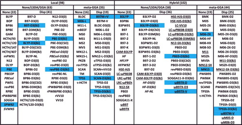
From the 200 benchmarked density functionals, 20 have been chosen for a thorough comparison within the body of this review, and these ‘featured’ functionals are listed in Table 3, along with a variety of details. The 20 functionals are categorised into five groups. The first group is a basic representation of Jacob's Ladder (without dispersion corrections), with SPW92 representing Rung 1 functionals (LSDA), PBE representing Rung 2 functionals (GGA), QTPSS representing Rung 3 functionals (meta-GGA), and B3LYP representing Rung 4 functionals (hybrid). They are primarily included for historic purposes, as well as to demonstrate the existence of a functional hierarchy when dispersion corrections are not vital (i.e. for thermochemistry and barrier heights). The functionals in the following four groups are dispersion-corrected local GGAs, dispersion-corrected local meta-GGAs (with the exception of M06-L), dispersion-corrected hybrid GGAs, and dispersion-corrected hybrid meta-GGAs (with the exception of M06-2X and MN15), respectively.

Table 3. Details for the 20 density functionals featured in the review, taken from the full list of 200 shown in Figure 13. The second column lists the number of parameters, counted according to the strategy in Figure 11. The third column indicates the percentage of exact exchange: a single, non-zero value indicates that the functional is a global hybrid (GH), while a range (e.g. 15–100) indicates that the functional is a range-separated hybrid (RSH), with the first value being the percentage of short-range exact exchange, and the second value being the percentage of long-range exact exchange (the value in parentheses is ω). The fourth column indicates the type of hybridisation. The fifth column indicates the ingredients (ρ, ∇ρ, and τ) contained in the functional. The sixth column indicates the type of dispersion correction, with D3(BJ) referring to Grimme's D3 method using the Becke– Johnson damping function, VV10 and rVV10 referring to the Vydrov and Van Voorhis nonlocal correlation functional and its revised version by Sabatini and co-workers, respectively, and CHG referring to the Grimme's D2 method using the Chai–Head–Gordon damping function.

Functional	#	cx · 100 (ω)	Hyb.	Ing.	Disp.	Year	Ref.
SPW92	0	0	None	LSDA	None	1992	23
PBE	0	0	None	GGA	None	1996	7
TPSS	0	0	None	meta-GGA	None	2003	8
B3LYP	3	20	GH	GGA	None	1993	9,29,35
PBE-D3(BJ)	3	0	None	GGA	D3(BJ)	2011	7,113
revPBE-D3(BJ)	4	0	None	GGA	D3(BJ)	2011	31,113
BLYP-D3(BJ)	4	0	None	GGA	D3(BJ)	2011	29,35,113
B97-D3(BJ)	12	0	None	GGA	D3(BJ)	2011	111,113
TPSS-D3(BJ)	3	0	None	meta-GGA	D3(BJ)	2011	8,113
SCAN-D3(BJ)	2	0	None	meta-GGA	D3(BJ)	2016	59,205
M06-L	34	0	None	meta-GGA	None	2006	62
B97M-rV	12	0	None	meta-GGA	rVV10	2017	124
PBE0-D3(BJ)	4	25	GH	GGA	D3(BJ)	2011	79,113
B3LYP-D3(BJ)	6	20	GH	GGA	D3(BJ)	2011	9,29,35,113
ωB97X-D	15	22.2–100 (0.2)	RSH	GGA	CHG	2008	119
ωB97X-V	10	16.7–100 (0.3)	RSH	GGA	VV10	2014	18
TPSSh-D3(BJ)	4	10	GH	meta-GGA	D3(BJ)	2011	84,113
M06-2X	29	54	GH	meta-GGA	None	2006	91
MN15	59	44	GH	meta-NGA	None	2016	94
ωB97M-V	12	15–100 (0.3)	RSH	meta-GGA	VV10	2016	20

Unless otherwise noted, the def2-QZVPPD basis set[206] was used without counterpoise corrections for all of the data-sets. A (99,590) grid (99 radial shells with 590 grid points per shell) was used for all of the data-sets except AE18 and RG10, for which a (500,974) grid was used. The SG-1 grid [207] was used to calculate the contribution from the VV10 nonlocal correlation functional[116] in all cases, except AE18 and RG10, for which a (75,302) grid was used. All of the calculations were performed with a development version of the Q-Chem 4 software package [208].

5. Comparative assessment of density functionals

Although only 20 of the 200 functionals are being specifically featured in this review, with data for such a large number of functionals at hand, it is certainly possible to make useful generalisations about the merits of using certain classes of functionals over others for specific types of interactions. To accomplish this goal, Figures 14–16 show box-and-whisker plots for the eight datatypes, with RMSDs for 188 of the 200 functionals separated into eight separate functional types: local or hybrid, GGA or meta-GGA, without or with dispersion corrections. The 12 omitted functionals are excluded either because they are severe outliers (HFLYP, HFPW92, PBEsol, PBEsol-D3(0), PBEsol-D3(BJ), SOGGA) or because they do not conform to any of the eight functional types (HF, HF-D3(0), HF-D3(BJ), HF-NL, SPW92, SVWN5). From the 188 remaining functionals, 18 are local GGAs without dispersion corrections (Local GGA None), 39 are local GGAs with dispersion corrections (Local GGA Disp), 16 are local meta-GGAs without dispersion corrections (Local mGGA None), 19 are local meta-GGAs with dispersion corrections (Local mGGA Disp), 19 are hybrid GGAs without dispersion corrections (Hybrid GGA None), 33 are hybrid GGAs with dispersion corrections (Hybrid GGA Disp), 19 are hybrid meta-GGAs without dispersion corrections (Hybrid mGGA None), and 25 are hybrid meta-GGAs with dispersion corrections (Hybrid mGGA Disp).

Figure 14. Box-and-whisker plots for eight classes of density functionals, covering the three datatypes (NCED, NCEC, and IE) that are most sensitive to the inclusion of dispersion corrections. Each plot is generated from functional RMSDs (in kcal/mol) for the specified datatype. The eight plots together contain data for 188 of the 200 functionals benchmarked in this review (the italicised functionals in Figure 13 are excluded), with each plot containing (from left to right) 18, 39, 16, 19, 19, 33, 19, and 25 functional RMSDs, respectively.

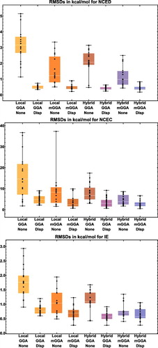
Figure 15. Box-and-whisker plots for eight classes of density functionals, covering the three datatypes (NCD, ID, and BH) that are most sensitive to the inclusion of exact exchange. Each plot is generated from functional RMSDs (in kcal/mol) for the specified datatype. The eight plots together contain data for 188 of the 200 functionals benchmarked in this review (the italicised functionals in Figure 13 are excluded), with each plot containing (from left to right) 18, 39, 16, 19, 19, 33, 19, and 25 functional RMSDs, respectively.

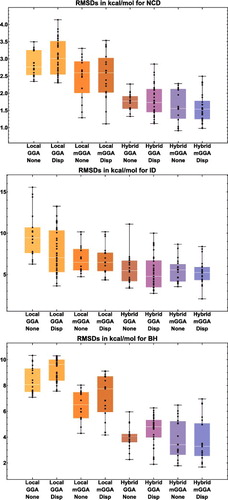
Figure 16. Box-and-whisker plots for eight classes of density functionals, covering the two datatypes (TCE and TCD) that are associated with bonded interactions. Each plot is generated from functional RMSDs (in kcal/mol) for the specified datatype. The eight plots together contain data for 188 of the 200 functionals benchmarked in this review (the italicised functionals in Figure 13 are excluded), with each plot containing (from left to right) 18, 39, 16, 19, 19, 33, 19, and 25 functional RMSDs, respectively.

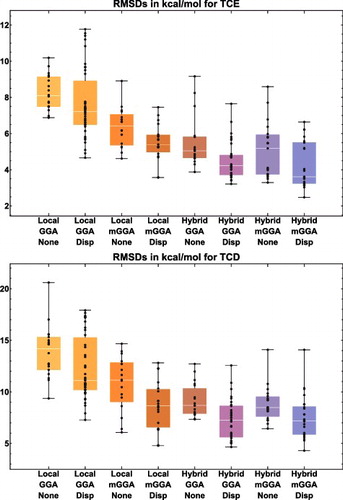
Perhaps the most interesting and optimistic figure is the one that represents the NCED category (top of Figure 14). The results clearly demonstrate that the dispersion corrections that are commonly utilised nowadays are extremely successful in improving the performance of density functionals for non-covalent interactions. Not only do the average RMSDs dramatically improve with the addition of dispersion corrections, the gap between the largest and smallest RMSD is significantly reduced. Not surprisingly, the local GGAs without dispersion corrections tend to perform the worst for NCED, while the best local meta-GGAs without dispersion corrections can approach the performance of a few dispersion-corrected functionals. The same is true for the non-dispersion-corrected hybrid GGA and hybrid meta-GGA functionals. Going from left to right, the smallest NCED RMSDs (in kcal/mol) across the eight different functional types are: 1.14 (GAM), 0.34 (BLYP-D3(BJ)), 0.50 (TM), 0.22 (B97M-rV), 0.47 (ωB97), 0.24 (ωB97X-V), 0.43 (M06-2X), and 0.18 (ωB97M-V). Therefore, within a certain functional type, the best non-dispersion-corrected functional cannot even approach the performance of the best dispersion-corrected functional. In some cases, the gap is larger (e.g. GAM is more than three times worse than BLYP-D3(BJ)), while ωB97 is only about two times worse than ωB97X-V. Ultimately, the figure is a testament to the successful efforts that have been devoted to the improvement of DFT for nonbonded interactions in the last decade.

For the non-covalent clusters in the NCEC datatype (middle of Figure 14), the improvements are almost as definitive as for NCED. For the most part, the local GGAs without dispersion corrections perform poorly, although the PKZB local meta-GGA functional is an extreme outlier in its class, with an RMSD of 37.31 kcal/mol. In comparison, its successor, TPSS, which was published only four years later, has an RMSD of 8.90 kcal/mol. Since the clusters in NCEC have much larger binding energies than the dimers in NCED, the RMSD scale for NCEC is about 10 times larger than that of NCED. Furthermore, even among the dispersion-corrected functionals, there is a larger gap between the largest and smallest RMSDs (relative to NCED). For example, the best and worst dispersion-corrected hybrid GGAs for NCEC are ωB97X-V (0.64 kcal/mol) and CAM-B3LYP-D3(0) (9.21 kcal/mol), respectively, while the best and worst dispersion-corrected hybrid GGAs for NCED are ωB97X-V (0.24 kcal/mol) and PBE0-D2 (0.63 kcal/mol), respectively. Considering the isomerisation energies in IE (bottom of Figure 14), the dispersion-corrected functionals improve upon their uncorrected counterparts as expected, with the functionals mostly exhibiting the trends mentioned for NCED and NCEC.

The next set of box-and-whisker plots highlight the importance of exact exchange. Figure 15 is structured identically to Figure 14 but contains information for the datatypes that are sensitive to electron delocalisation, namely, NCD, ID, and BH. For these three categories, it is straightforward to conclude that the hybrid functionals perform better than the local functionals, on average. The results for NCD are interesting, since the dispersion-corrected functionals tend to perform worse than those without dispersion corrections. This is particularly true for the local GGAs, and is attributed to the fact that these functionals tend to greatly overbind complexes that exhibit severe electron delocalisation. For example, for an electron-poor/hemibonded system such as H₂O—F, BLYP predicts a binding energy of -18.87 kcal/mol, compared to the reference of -3.83 kcal/mol. Naturally, BLYP-D3(BJ) can only do worse, with a binding energy of -19.45 kcal/mol. Therefore, it is not surprising that the dispersion-corrected local GGAs, as a whole, tend to perform worse than their uncorrected counterparts. Furthermore, the inclusion of the kinetic energy density tends to help only slightly for the NCD datatype, on average, although a few local meta-GGAs can approach the performance of the hybrids.

While the results for the ID datatype (middle of Figure 15) are the least telling, it is still evident that the hybrids outperform the local functionals, and that the local GGAs without dispersion corrections perform worse than the rest. On the other hand, the distinction between the local and hybrid functionals is very prominent for barrier heights (bottom of Figure 15). With BH, the best local GGAs are worse than the worst hybrids, and this result supports the conventional wisdom that hybrids should be used for kinetics, if computationally feasible. Furthermore, it has been repeatedly reported in the literature that local meta-GGAs significantly improve upon local GGAs for barrier heights, and this fact is confirmed in Figure 15. Some of the best local meta-GGAs can even approach the performance of a few hybrids. However, even the best local meta-GGAs are no match for the best hybrids. Going from left to right, the smallest BH RMSDs (in kcal/mol) across the eight different functional types are: 7.09 (N12), 7.56 (OLYP-D3(0)), 4.29 (MN12-L), 4.16 (MN12-L-D3(BJ)), 2.26 (SOGGA11-X), 1.89 (SOGGA11-X-D3(BJ)), 1.78 (M08-SO), and 1.68 (ωB97M-V). Thus, the best local GGAs still have RMSDs larger than 7 kcal/mol, local meta-GGAs can approach the 4 kcal/mol barrier, while hybrids can comfortably beat the 2 kcal/mol mark.

Finally, the performance of the 188 functionals is summarised for thermochemistry in Figure 16. For TCE (top of Figure 16), the functionals tend to conform to Jacob's Ladder, with the local meta-GGAs outperforming the local GGAs, and the hybrids outperforming the local functionals. Based on the averages RMSDs, the hybrids with dispersion corrections tend to perform best, followed by the hybrids without dispersion corrections. It is interesting that among the local functionals, dispersion-corrected GGAs outperform their uncorrected counterparts, and dispersion-corrected meta-GGAs outperform their uncorrected counterparts. For the difficult bonded interactions in TCD, the best possible RMSD is nearly a factor of 2 larger than the best TCE RMSD, and this reflects the difficulty of the interactions classified in the TCD datatype. However, for the most part, the behavior of the functionals for TCE is mimicked in the TCD datatype.

5.1. Overall performance of 20 leading functionals

In order to facilitate the comparison of the 20 featured functionals across the database of nearly 5000 data points, color-coded (by column) tables will be used (Figures 17–26). The rows of these tables are populated by density functionals, while the columns represent either datatypes (e.g. NCED) or data-sets (e.g. S22). At the bottom of each table, the minimum RMSD from across all 200 benchmarked functionals is listed (in the row labelled ‘Minimum’), along with the name of the corresponding functional (in the row labelled ‘Best’). For example, according to Figure 18, LC-VV10 has the smallest RMSD (0.12 kcal/mol) for the NBC10 data-set, while from the featured functionals, ωB97M-V performs best with an RMSD of 0.16 kcal/mol.

Figure 17. RMSDs in kcal/mol for the eight datatypes (as well as 81 equilibrium bond lengths (EBL in Ångström) and 81 equilibrium binding energies (EBE in kcal/mol)) for the 20 density functionals featured in this review, along with the minimum RMSD from across all 200 benchmarked functionals, and the name of the corresponding functional. The eight datatypes contain 1744, 243, 91, 755, 155, 947, 258, and 206 data points, respectively. NCED stands for non-covalent dimers (easy), NCEC stands for non-covalent clusters (easy), NCD stands for non-covalent dimers (difficult), IE stands for isomerisation energies (easy), ID stands for isomerisation energies (difficult), TCE stands for thermochemistry (easy), TCD stands for thermochemistry (difficult), and BH stands for barrier heights. ‘Difficult’ interactions involve either self-interaction error or strong correlation, while ‘easy’ interactions are not significantly characterised by either.

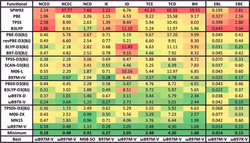
Figure 18. RMSDs in kcal/mol for the 18 data-sets that belong to the NCED datatype. Results for the 20 density functionals featured in this review are presented, along with the minimum RMSD from across all 200 benchmarked functionals, and the name of the corresponding functional. The 1744 interactions that are categorised as NCED are conventional, closed-shell, non-covalent dimers.

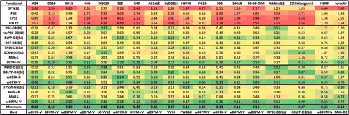
Figure 17 contains a summary of the performance of the 20 functionals, with RMSDs for the eight datatypes, as well as for the two categories (EBL and EBE) that pertain to non-covalent dimer equilibrium properties extracted from the 81 non-rare-gas dimer PECs mentioned in Section 4.1. As a reminder, these PECs are found in the BzDC215, NBC10, and S66x8 data-sets in NCED. Considering the first set of four functionals, their performance for standard thermochemistry (TCE) and barrier heights (BH) is fascinating, as it follows the hierarchy dictated by Jacob's Ladder. Naturally, the LSDA functional, SPW92, has the worst performance for the bonded interactions in TCE, with an RMSD of over 42 kcal/mol. With the help of the density gradient, PBE slashes the RMSD of its Rung 1 relative by more than a factor of 4.5 (9.22 kcal/mol), while TPSS yields further substantial improvement (5.94 kcal/mol). Although the improvement offered by B3LYP over PBE is quite significant, it is noteworthy that B3LYP (a global hybrid GGA) and TPSS (a local meta-GGA) tend to perform quite similarly for TCE. This result supports the notion that meta-GGA functionals can reach the accuracy of hybrid functionals in certain cases, at a much lower computational cost. The same trend can be seen for the difficult bonded interactions in TCD, and for this particular set of 258 data points, TPSS actually manages to slightly outperform B3LYP. However, for the barrier heights, while the distinction between SPW92 and either PBE or TPSS is substantial (factor of 2), B3LYP is greatly aided by its 20% mixing of exact exchange, and comfortably outperforms the local functionals in a category where exact exchange is known to be of utmost importance. Since these functionals are not equipped to deal with non-covalent interactions and isomerisation energies, their performance for the five associated datatypes (NCED, NCEC, NCD, IE, and ID) will not be discussed.

From the four dispersion-corrected local GGA functionals, BLYP-D3(BJ) is the best performer for non-covalent interactions, with the smallest RMSDs for both NCED (0.34 kcal/mol) and NCEC (2.18 kcal/mol), while B97-D3(BJ) performs best for thermochemistry and barrier heights, most likely due to their emphasis in its semi-empirical construction. Compared to the best possible result for the isomerisation energies in IE (0.27 kcal/mol), the local GGAs tend to perform poorly, with BLYP-D3(BJ) having the smallest RMSD of the four, at 0.68 kcal/mol. Comparing PBE-D3(BJ) to PBE demonstrates the importance of the dispersion correction for NCED and IE, as well as for the equilibrium properties. The improvement for NCED is expected, since this datatype contains a variety of data-sets that contain dispersion-bound complexes. However, NCEC is mostly populated by hydrogen-bonded clusters, and the addition of the dispersion correction to PBE necessarily deteriorates agreement with the reference, as PBE is already overbound for water clusters, and the addition of a dispersion tail can only lead to more binding. Comparing revPBE-D3(BJ) and PBE-D3(BJ) for thermochemistry is relevant, as the former was constructed by fitting a linear parameter in the PBE exchange functional to atomisation energies. Accordingly, revPBE-D3(BJ) outperforms PBE-D3(BJ) significantly for both of the thermochemistry datatypes. However, it is noteworthy that the performance for BH is not significantly improved, further confirming that exact exchange is necessary to give such functionals higher accuracy.

Moving on to the local meta-GGA functionals in the third group of Figure 17, TPSS-D3(BJ) represents the first successful non-empirical meta-GGA by Perdew and co-workers, while SCAN-D3(BJ) is Perdew's most recent non-empirical meta-GGA. M06-L is arguably the most successful local Minnesota functional, and B97M-rV is a dispersion-corrected (rVV10) meta-GGA density functional developed via a partial combinatorial search of the meta-GGA functional space. Comparing the two dispersion-corrected non-empirical local meta-GGAs, SCAN-D3(BJ) is an improvement over TPSS-D3(BJ) for isomerisation energies, thermochemistry, and barrier heights. Unfortunately, this comes at the cost of heavily degraded performance for non-covalent interactions, as TPSS-D3(BJ) is nearly 30% better than SCAN-D3(BJ) for NCED, and the RMSD of SCAN-D3(BJ) for non-covalent clusters is the second largest (after SPW92) from the 20 functionals in Figure 17, at 9.18 kcal/mol. The underlying reason for the poor performance of SCAN-D3(BJ) for NCEC is its tendency to greatly overbind hydrogen bonds. As an example, the reference binding energy of the water dimer in the S22 data-set is -4.99 kcal/mol, and SCAN itself binds the dimer at -5.41 kcal/mol, while SCAN-D3(BJ) binds it at -5.54 kcal/mol. A second relevant example is the formic acid dimer, which has two hydrogen bonds. The S22 reference is -18.75 kcal/mol, while SCAN and SCAN-D3(BJ) give binding energies of -20.80 and -21.25 kcal/mol, respectively. Considering the prism water hexamer from H2O6Bind8 as a larger example, the reference binding energy is only -48.31 kcal/mol, while SCAN-D3(BJ) predicts a value of -55.47 kcal/mol. Adding the semi-empirical local meta-GGAs into the mix, B97M-rV is a clear winner for the ‘easy’ non-covalent interactions and isomerisation energies, as well as for thermochemistry and barrier heights. However, while its performance for NCED, NCEC, and IE is either the best possible (across all 200 functionals) or very close to it, there is room for improvement for thermochemistry and barrier heights with the addition of exact exchange. Furthermore, none of the local functionals discussed thus far are able to approach the accuracy possible for the NCD and ID datatypes.

Of the four dispersion-corrected hybrid GGA density functionals, the first two (PBE0-D3(BJ) and B3LYP-D3(BJ)) are global hybrids with 25% and 20% global exact exchange, respectively, while the latter two (ωB97X-D and ωB97X-V) are range-separated hybrids that tend to 100% exact exchange in the long range and have 22.2% and 16.7% exact exchange in the short range, respectively. First, it is of interest to compare PBE0-D3(BJ) and PBE-D3(BJ), since the hybridisation is the only feature that sets them apart. Interestingly, the performance for NCED is nearly identical, while the hybrid is slightly better for the non-covalent clusters. However, for the categories where exact exchange is vital (NCD, ID, and BH), PBE0-D3(0) represents a significant enhancement over its local counterpart, with improvements of 40%, 30%, and 50%, respectively. The performance for thermochemistry is improved by a factor of 2 upon hybridisation, and there is also a non-negligible change in the performance of IE (about 15%). It is comforting that the same conclusions apply almost exactly when one compares B3LYP-D3(BJ) to its local counterpart, BLYP-D3(BJ). With regards to B3LYP-D3(BJ), it is remarkable that its RMSD for NCED is only 0.31 kcal/mol, as it outperforms all of the 20 functionals, excluding the three combinatorially optimised ones (B97M-rV, ωB97X-V, and ωB97M-V). Considering the range-separated hybrid GGAs, ωB97X-V is significantly better than ωB97X-D for non-covalent interactions and isomerisation energies, yet quite similar for thermochemistry and barrier heights. This indicates that these functionals are perhaps near the limit approachable by a well-rounded hybrid GGA for bonded systems and kinetics, while the distinction in nonbonded interactions and isomerisation energies potentially highlights the merits of VV10 over DFT-D.

Finally, the last set of four functionals represent the hybrid meta-GGAs, with three global hybrids (TPSSh-D3(BJ), M06-2X, and MN15) and a range-separated hybrid (ωB97M-V). Once again, it is interesting to compare TPSSh-D3(BJ) and TPSS-D3(BJ) to assess the importance of hybridisation. Perhaps due to the small fraction of exact exchange (10%), as well as the fact that a local meta-GGA like TPSS-D3(BJ) is better equipped (than a GGA) to handle electron delocalisation due to the presence of the kinetic energy density, the difference between these two functionals is not as drastic as the difference for equivalent GGAs (e.g. PBE0-D3(BJ) and PBE-D3(BJ)). For example, while PBE0-D3(BJ) is 40% better than PBE-D3(BJ) for NCD, TPSSh-D3(BJ) is slightly more than 15% better than TPSS-D3(BJ). The same result can be seen for BH, where the improvement is 50% for the PBE-based pair, yet only 25% for the TPSS-based pair. Moving on to the two hybrid meta-GGA Minnesota functionals, M06-2X is perhaps the most popular hybrid Minnesota functional, while MN15 is a recent attempt at maintaining the performance of M06-2X for single-reference main-group thermochemistry, while improving its description of multi-reference cases. For non-covalent interactions, the two are quite similar, with M06-2X being slightly better for the dimers in NCED and MN15 being slightly better for clusters, while both are equivalent for NCD. Similarly, M06-2X is clearly better (by 30%) for the isomerisation energies in IE, while MN15 is 30% better for the isomerisation energies in ID. For standard bonded interactions (like the ones in TCE), M06-2X has the edge over MN15, while for the (mostly) multi-reference cases in TCD, MN15 is slightly better (as intended). Finally, MN15 significantly improves over M06-2X for BH, making it one of the more promising Minnesota functionals in recent years. However, compared to the performance that is actually possible from a hybrid meta-GGA, MN15 falls far short of the ωB97M-V density functional. For the non-covalent dimers in NCED and the isomerisation energies in IE, ωB97M-V performs more than 2.5 times better than MN15, while for the clusters, it performs nearly 4 times better than MN15. ωB97M-V is also 30% more accurate for thermochemistry, and slightly more accurate for BH (about 15%). In fact, the only category in which MN15 outperforms ωB97M-V is NCD, and this is primarily due to the fact that MN15 has 44% exact exchange, and ωB97M-V only has 15% short-range exact exchange.

In order to discuss the eight specific datatypes in a practical and concise manner, the remainder of Section 5 is split into four subsections that pertain to non-covalent interactions, isomerisation energies, thermochemistry, and barrier heights. Within each subsection, the relevant datatypes will be discussed by making specific references to only a few of the associated data-sets. For example, since the NCED datatype itself has been discussed already, Section 5.2 will assess the performance of the functionals on specific NCED data-sets, such as S22 or S66.

5.2. Non-covalent interactions

Interest in non-covalent interactions has skyrocketed in the past decade, and it is therefore not surprising that of the 82 data-sets that are categorised into datatypes, 35 of them are associated with non-covalent interactions. Figures 18–20 cover the three datatypes that pertain to non-covalent interactions: NCED, NCEC, and NCD. Furthermore, Figure 21 covers equilibrium properties for the four data-sets that contain PECs: BzDC215, NBC10, RG10, and S66x8.

Figure 19. RMSDs in kcal/mol for the 12 data-sets that belong to the NCEC datatype. Results for the 20 density functionals featured in this review are presented, along with the minimum RMSD from across all 200 benchmarked functionals, and the name of the corresponding functional. The 243 interactions that are categorised as NCEC are conventional, closed-shell, non-covalent clusters.

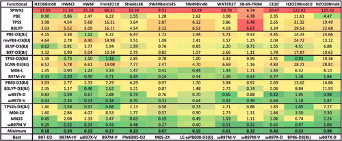
Figure 20. RMSDs in kcal/mol for the five data-sets that belong to the NCD datatype. Results for the 20 density functionals featured in this review are presented, along with the minimum RMSD from across all 200 benchmarked functionals, and the name of the corresponding functional. The 91 interactions that are categorised as NCD are either open-shell non-covalent dimers or non-covalent dimers characterised by significant electron delocalisation.

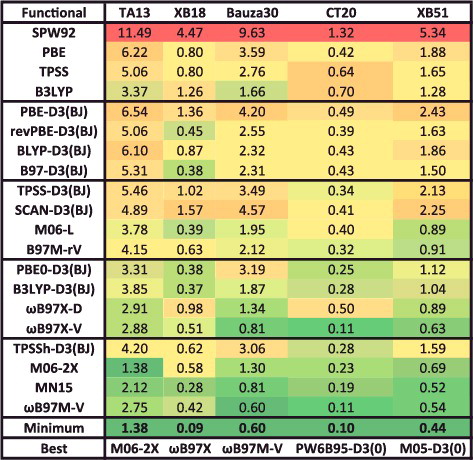
Figure 21. RMSDs for equilibrium bond lengths (EBL) in Ångström and equilibrium binding energies (EBE) in kcal/mol for four data-sets that contain potential energy curves. Results for the 20 density functionals featured in this review are presented, along with the minimum RMSD from across all 200 benchmarked functionals, and the name of the corresponding functional.

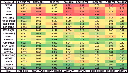
Starting with the non-covalent interactions in NCED (Figure 18), an effective data-set that covers various types of interactions (hydrogen-bonded, dispersion-bound, mixed) as well as a variety of geometric configurations (compressed, equilibrium, stretched) is S66x8. This data-set contains a total of 528 data points, and is comprised of 66 non-covalent dimer PECs with eight points per curve, starting from 90% of the equilibrium separation and stretching out to 200% of the equilibrium separation. Therefore, it is an invaluable data-set for acquiring a general idea about the performance of density functionals for conventional non-covalent interactions. As a point of reference, the root-mean-square of the 528 interaction energies in S66x8 is only 5.57 kcal/mol. Looking at the four ‘historic’ functionals, it is clear that they are incapable of handling such systems, as their RMSDs are in excess of 2 kcal/mol. From the local functionals, B97M-rV and BLYP-D3(BJ) perform remarkably well, with RMSDs of 0.17 and 0.21 kcal/mol, respectively. In comparison, both SCAN-D3(BJ) and M06-L have RMSDs in excess of 0.5 kcal/mol, while the rest of the local functionals (besides PBE and TPSS) have RMSDs between 0.3 and 0.45 kcal/mol. Most of the hybrids do not necessarily perform better than the local functionals, with both PBE0-D3(BJ) and TPSSh-D3(BJ) performing nearly identically to their local counterparts. However, ωB97M-V, with an outstandingly small RMSD of 0.11 kcal/mol, is not only the best of the 20 functionals in Figure 18, but the best across all 200 functionals considered in this benchmark. In comparison, MN15 has an RMSD that is more than 4 times larger. Compared to its predecessor, ωB97X-V, ωB97M-V represents an improvement of nearly a factor of 2 on the S66x8 data-set.

A data-set from NCED that deals primarily with hydrogen bonds is HB49[170–172], which is comprised of 49 hydrogen-bonded complexes from a recent benchmark by Boese. The concluding remarks of the article[172] titled ‘Density Functional Theory and Hydrogen Bonds: Are We There Yet?’ stated that none of the tested density functionals were able to outperform MP2 at the CBS limit, which had an RMSD of around 0.3 kcal/mol. Using this value as a guideline, it is evident that of the 20 functionals in Figure 18, only ωB97X-V and ωB97M-V are able to surpass this mark. ωB97X-V performs nearly identically to MP2/CBS, while ωB97M-V performs more than 20% better for a category where MP2 is already a trustworthy choice. All of the local GGA functionals have RMSDs greater than 0.6 kcal/mol, but it is noteworthy that BLYP-D3(BJ) once again performs best in its class. Of the local meta-GGAs, only B97M-rV (0.44 kcal/mol) is able to break the 0.5 kcal/mol RMSD barrier, but its performance falls nearly a factor of 2 short of its hybrid cousin, ωB97M-V. While the hybrid GGAs mostly improve upon the local GGAs, only the two range-separated functionals approach the performance of MP2, with ωB97X-D (0.37 kcal/mol) falling short of ωB97X-V (0.29 kcal/mol). Finally, the spread for the hybrid meta-GGAs is rather large, with the non-empirical TPSSh-D3(BJ) affording an RMSD of 0.73 kcal/mol, and the two Minnesota functionals, with RMSDs slightly over 0.55 kcal/mol, performing similar to B3LYP-D3(BJ). Overall, ωB97M-V is the best performer across all 200 benchmarked functionals for HB49.

The final data-set from NCED that will be discussed is AlkBind12, as it represents complexes dominated by the dispersion energy: saturated and unsaturated hydrocarbon dimers. Interestingly, the RMSDs of the ‘historic’ functionals display a reverse Jacob's Ladder behaviour, with the LSDA (SPW92) performing best and the hybrid (B3LYP) performing worst. Nevertheless, these functionals are not meant to be used in their uncorrected form, and the performance of their dispersion-corrected counterparts remains to be seen. From the dispersion-corrected local GGAs, PBE-D3(BJ) performs remarkably well, with an RMSD of only 0.15 kcal/mol, while the others have RMSDs between 0.2 and 0.4 kcal/mol. Surprisingly, none of the meta-GGAs perform as well as PBE-D3(BJ), with SCAN-D3(BJ) placing first with an RMSD of 0.23 kcal/mol, followed by B97M-rV (0.27 kcal/mol). Moving on to the hybrid GGAs, PBE0-D3(BJ) further improves upon PBE-D3(BJ), with an RMSD of 0.12 kcal/mol, which exactly matches the RMSD of ωB97X-V. In stark contrast, however, the predecessor of ωB97X-V, ωB97X-D, performs poorly for the AlkBind12 data-set, with an RMSD of 1 kcal/mol. As for the hybrid meta-GGAs, TPSSh-D3(BJ) barely improves over TPSS-D3(BJ), while the popular M06-2X functional has an RMSD of 0.30 kcal/mol. Compared to the good performance of M06-2X, MN15 performs poorly for this data-set, with an RMSD that is nearly 4 times larger, at 1.18 kcal/mol. Again, ωB97M-V performs laudably, with an RMSD (0.13 kcal/mol), that is only 0.02 kcal/mol away from the best performer within the 200 functionals.

Progressing to the non-covalent clusters in NCEC (Figure 19), a data-set representative of water clusters is Shields38, as it contains binding energies up to the water decamer. The RMS of the binding energies in this data-set is 51.54 kcal/mol, so the corresponding functional RMSDs will naturally be larger than for the NCED data-sets previously discussed. From the ‘historic’ functionals, PBE is clearly the best performer, with a promising RMSD of 1.55 kcal/mol, while the LSDA has a significantly larger RMSD of 33.36 kcal/mol. While PBE performs well, PBE-D3(BJ) overbinds the water clusters, with an RMSD (6.47 kcal/mol) that is more than four times larger than that of PBE. The second best-performing local GGA is BLYP-D3(BJ), which performs on par with PBE. From the local meta-GGAs, M06-L is able to slightly outperform PBE, with an RMSD of 1.47 kcal/mol, while B97M-rV (0.45 kcal/mol) performs more than three times better than M06-L. While TPSS-D3(BJ) actually improves upon TPSS, it is unable to match the performance of PBE. However, TPSS-D3(BJ) still manages to outperform SCAN-D3(BJ) by a factor of nearly 3. While PBE0-D3(BJ) slightly ameliorates the overbinding of PBE-D3(BJ), its RMSD is still more than 2.5 times larger than that of PBE. Both of the range-separated hybrid GGAs perform very well, with RMSDs around 0.7 kcal/mol, outperforming PBE by a factor of about 2. ωB97M-V, with an RMSD of 0.48 kcal/mol, performs nearly as well as its local counterpart B97M-rV, while MN15 (0.63 kcal/mol) outperforms M06-2X (1.77 kcal/mol) by nearly a factor of 3.

The TA13 data-set in NCD (Figure 20) attempts to probe weak interactions between radicals and their environment. As such, SIE plagues the performance of local functionals for these complexes, and hybrids with high fractions of exact exchange are desired. Accordingly, the best performer across all 200 density functionals is M06-2X (54% exact exchange), which manages an RMSD of 1.38 kcal/mol. B3LYP-D3(BJ), which has about 2.7 times less exact exchange than M06-2X, performs about 2.7 times worse than M06-2X. Even ωB97M-V, due to its small fraction of 15% short-range exact exchange, struggles for this data-set (two times worse than M06-2X), but outperforms ωB97X-V and B97M-rV, as expected. The four ‘historic’ functionals are once more ordered in accordance with Jacob's Ladder, with the hybrid B3LYP having the smallest RMSD of 3.37 kcal/mol, and SPW92 having the largest RMSD (11.49 kcal/mol). None of the local GGAs manage RMSDs below 5 kcal/mol, while only one of the meta-GGAs (M06-L) manages an RMSD below 4 kcal/mol. The better performance of the hybrids, however, clearly indicates that the interactions in this data-set are prone to SIE, as the hybrid GGAs have RMSDs around 3 kcal/mol, and the hybrid meta-GGAs perform slightly better, with RMSDs mostly in the vicinity of 2 kcal/mol.

Accurate modeling of potential energy surfaces is of utmost importance in many computational chemistry applications, and the performance of the 20 featured functionals is assessed on four data-sets of non-covalent dimer PECs in Figure 21. Since the S66x8 data-set contains a total of 66 PECs, it will be used to assess the performance of the functionals. For the EBLs, the ‘historic’ functionals perform badly (as expected), with RMSDs around 0.2 Å. The dispersion-corrected local GGAs greatly improve upon the four aforementioned functionals, with three of them managing RMSDs around 0.05 Å  and BLYP-D3(BJ) affording an impressive RMSD of 0.027 Å. TPSS-D3(BJ) performs worse than the four dispersion-corrected local GGAs, while B97M-rV, M06-L, and SCAN-D3(BJ) perform well, with RMSDs under 0.035 Å. B97M-rV manages to slightly outperform BLYP-D3(BJ), with an RMSD of 0.021 Å, while M06-L matches the performance of BLYP-D3(BJ). Surprisingly, the dispersion-corrected hybrid GGAs are only slightly better than the dispersion-corrected local GGAs, with B3LYP-D3(BJ) putting in an impressive performance and affording an RMSD of 0.022 Å. From the hybrid meta-GGAs, TPSSh-D3(BJ) performs rather poorly, and offers no improvement over its local counterpart, while M06-2X also ends up with an RMSD larger than 0.07 Å. MN15 cuts the RMSD of M06-2X by a factor of 2, while the RMSD of ωB97M-V is more than 4 times smaller than that of MN15 (and the smallest from across all 200 functionals). For the most part, these trends carry over to the EBEs, with a few exceptions. First, while ωB97X-V is about average for the bond lengths, it manages the best performance across all 200 functionals for the S66x8 EBEs, while B3LYP-D3(BJ), which was impressive for the bond lengths, is not as accurate for the binding energies. Second, while M06-2X performed about a factor of 2 worse than MN15 for the bond lengths, it performs about a factor of 2 better for the binding energies.

5.3. Isomerisation energies

The ability to accurately and efficiently determine relative conformational energies is valuable in many applications of computational chemistry. Therefore, many data-sets that address this issue have been published in the past decade, and the IE (Figure 22) and ID (Figure 23) datatypes together contain 17 isomerisation energy data-sets.

Figure 22. RMSDs in kcal/mol for the 12 data-sets that belong to the IE datatype. Results for the 20 density functionals featured in this review are presented, along with the minimum RMSD from across all 200 benchmarked functionals, and the name of the corresponding functional. The 755 interactions that are categorised as IE are conventional, closed-shell, isomerisation energies.

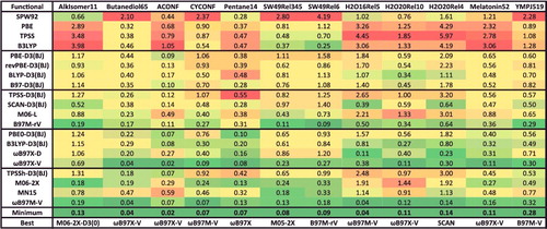
Figure 23. RMSDs in kcal/mol for the five data-sets that belong to the ID datatype. Results for the 20 density functionals featured in this review are presented, along with the minimum RMSD from across all 200 benchmarked functionals, and the name of the corresponding functional. The 155 interactions that are categorised as ID are isomerisation energies characterised by significant electron delocalisation.

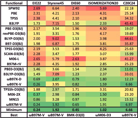
From the IE datatype, the Butanediol65 data-set will be analysed as a representative of conformational equilibria of organic molecules. The RMS of the relative energies in this data-set is small, only 2.89 kcal/mol. The smallest RMSD of all 200 benchmarked functionals is 0.04 kcal/mol, and belongs to ωB97X-V. Coincidentally, ωB97M-V has an RMSD of only 0.04 kcal/mol as well, representing an error of about 2%. After these two functionals, the next best (from the 20 featured) is B97M-rV, with an RMSD of 0.17 kcal/mol. The local GGAs consistently have a mediocre performance, with RMSDs between 0.3 and 0.45 kcal/mol, while three of the five local meta-GGAs are consistently better, with RMSDs between 0.15 and 0.3 kcal/mol. SCAN-D3(BJ), however, performs uncharacteristically poor for its class, with an RMSD of 0.38 kcal/mol, and is similar to TPSS without dispersion corrections. The addition of exact exchange tends to help, as the dispersion-corrected hybrid GGAs are consistently better than the dispersion-corrected local GGAs, and most of the hybrid meta-GGAs are better than the local meta-GGAs (with the exception of MN15, which performs on par with the local GGAs, with a rather large RMSD of 0.47 kcal/mol).

Before moving on to the ‘difficult’ isomerisation energies, it is useful to look at the performance of these functionals for a class other than organic molecules. Therefore, the H2O16Rel5 data-set by Xantheas and co-workers will be used to assess the ability of the functionals for predicting the proper relative ordering of large water clusters. In this specific case, the relative energies of five low-lying water 16-mer structures were computed at the CCSD(T)/aug-cc-pVTZ level of theory [146]. The best functional, by far, is ωB97M-V, with an impressive RMSD of only 0.04 kcal/mol. Only one other functional is able to approach the performance of ωB97M-V, and that is ωB97X-D with an RMSD of 0.11 kcal/mol. Three other functionals have RMSDs below 0.5 kcal/mol: ωB97X-V, SCAN-D3(BJ), and B97M-rV. The rest of the functionals perform poorly, with some even yielding RMSDs larger than 2 kcal/mol (M06-L, TPSSh-D3(BJ), and TPSS-D3(BJ)). Surprisingly, the LSDA functional manages to outperform 13 of the functionals in Figure 22 for this data-set.

The DIE60 data-set by Yu and Karton contains 60 conjugated → non-conjugated diene isomerisation energies, and will serve as the representative data-set from the ID datatype due to the significant presence of SIE. The ‘historic’ functionals adhere to Jacob's Ladder once more, with B3LYP exhibiting the smallest RMSD of 1.50 kcal/mol. B3LYP-D3(BJ) performs about 20% better than B3LYP for this data-set, indicating that the inclusion of a dispersion correction plays a non-negligible role. The local GGAs all perform worse than B3LYP, while the local meta-GGAs perform worse than the local GGAs on average, which is unexpected. Following expectations, however, most of the hybrids improve upon the local functionals, with five of them breaking the 1 kcal/mol barrier, including M06-2X and MN15. The two range-separated hybrid GGAs perform similarly, with RMSDs around 0.8 kcal/mol, while ωB97M-V manages the smallest RMSD (0.65 kcal/mol) from the 20 functionals. The smallest RMSD across all 200 functionals (0.45 kcal/mol), however, is reserved for BMK-D3(0), which has 42% global exact exchange.

5.4. Thermochemistry

While KS-DFT was formally established more than 50 years ago, the popularity that DFT enjoys today began to grow only in the early 1990s. The first comprehensive testing of density functionals on molecular systems was performed by Becke on the G1 atomisation energy test set [209–211], and further tests quickly followed by Pople et al. [212] using the BLYP functional (the dispersion-corrected version of which is part of the 20 functionals featured here). Nonetheless, DFT first achieved its popularity due to its remarkable performance for atomisation energies, and these types of systems are covered in the TCE datatype. Of the 15 TCE data-sets in Figure 24, two deal with atomisation energies: TAE140nonMR and AlkAtom19. Since the former is comprised of small molecules, and similar data-sets have been used in the construction of most of the semi-empirical functionals contained in this benchmark, the AlkAtom19 data-set which contains atomisation energies for linear and branched alkanes up to octane will be used as a representative from TCE.

Figure 24. RMSDs in kcal/mol for the 15 data-sets that belong to the TCE datatype. Results for the 20 density functionals featured in this review are presented, along with the minimum RMSD from across all 200 benchmarked functionals, and the name of the corresponding functional. The 947 interactions that are categorised as TCE are conventional, single-reference bonded interactions.

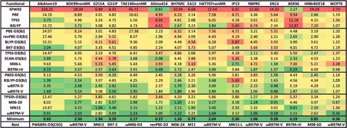
With an RMS of 1829.31 kcal/mol, the atomisation energies in AlkAtom19 are significantly larger in magnitude than those found in standard atomisation energy test sets. Therefore, functional RMSDs that are in the vicinity of a few kcal/mol should be acceptable. Of the 20 featured functionals, only 8 manage RMSDs under 5 kcal/mol. The remaining 12 have RMSDs that range from 8.02 kcal/mol (M06-2X) to 14.67 kcal/mol (MN15) to 228.25 kcal/mol (SPW92). Strangely, while B3LYP performs poorly with an RMSD of 15.72 kcal/mol, B3LYP-D3(BJ) manages an RMSD of only 1.39 kcal/mol, simply due to the fact that the dispersion correction makes up for the underbinding of B3LYP by lowering the energy of the molecules but not the atoms. Only two functionals manage RMSDs under 1 kcal/mol: B97M-rV (0.72 kcal/mol) and ωB97M-V (0.91 kcal/mol).

The HAT707nonMR data-set from W4-11 contains 505 single-reference heavy-atom transfer reaction energies, a good alternative to atomisation energies. Unlike with the AlkAtom19 data-set, the performance of the ‘historic’ functionals for HAT707nonMR is in accordance with expectation, as SPW92 (12.54 kcal/mol), PBE (7.58 kcal/mol), TPSS (6.05 kcal/mol), and B3LYP (3.84 kcal/mol) perform successively better. The local GGAs have RMSDs between 5 and 8 kcal/mol, while the local meta-GGAs significantly improve upon the GGAs, with RMSDs between 3.5 and 6.1 kcal/mol. Besides PBE0-D3(BJ), the hybrid GGAs perform very similarly, with RMSDs around 3.75 kcal/mol. True to expectation, the hybrid meta-GGAs exhibit the best performance from the 20 functionals, with M06-2X affording an RMSD of 3.27 kcal/mol. Only ωB97M-V is able to outperform M06-2X, with an RMSD of 2.64 kcal/mol.

Despite the fact that multi-reference systems are not the strong suit of most existing approximate Kohn–Sham density functionals, it is nevertheless interesting to take a look at the performance of these functionals for a data-set that deals with such systems (Figure 25). The TAE140MR data-set of 16 multi-reference atomisation energies is a suitable candidate. The ‘historic’ functionals strongly display their true positions on Jacob's Ladder, with SPW92 having an RMSD of 74.81 kcal/mol and B3LYP having an RMSD of 5.60 kcal/mol. The local GGAs perform poorly overall, with RMSDs in excess of 10 kcal/mol, while the local meta-GGAs are a definite improvement, with RMSDs between 5 and 13 kcal/mol. Hybrid functionals with low percentages of exact exchange (TPSS-D3(BJ), B3LYP-D3(BJ), and PBE0-D3(BJ)) perform very well, with RMSDs around or below 4 kcal/mol. The range-separated hybrids suffer due to the increasing fraction of exact exchange with interelectronic distance, and manage RMSDs between 5 and 6 kcal/mol. However, they still perform better than M06-2X (8.49 kcal/mol), which has 54% global exact exchange. Due to its design strategy, MN15 (5.63 kcal/mol), despite having 44% global exact exchange, improves greatly upon M06-2X. MN15 still falls short of ωB97M-V (5.28 kcal/mol), a minimally parameterised and transferable functional with no emphasis on multi-reference systems in its design principles.

Figure 25. RMSDs in kcal/mol for the seven data-sets that belong to the TCD datatype. Results for the 20 density functionals featured in this review are presented, along with the minimum RMSD from across all 200 benchmarked functionals, and the name of the corresponding functional. The 258 interactions that are categorised as TCD are bonded interactions that are either very sensitive to self-interaction error or significantly multi-reference in nature.

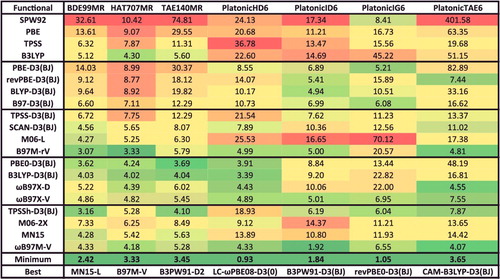
5.5. Barrier heights

While barrier heights were not heavily present in the benchmark data-sets used in the early days of DFT, near the turn of the century, interest in better density functionals for kinetics sparked a flurry of functional development with an emphasis on BH performance. One of the first such functionals, MPW1K [213], was a semi-empirical global hybrid GGA functional by Truhlar et al., with 42.8% exact exchange, a significant yet deliberate departure from the conventional 20% found in the B3-type functionals. Other similar endeavours [87,214] by the Truhlar group produced the BB1K (42% exact exchange), XB1K (43% exact exchange), MPWB1K (44% exact exchange), and PWB6K (46% exact exchange) global hybrid meta-GGA functionals, while Boese and Martin developed the global hybrid GGA B97-K functional and the global hybrid meta-GGA BMK functional, both with 42% exact exchange. Before discussing the performance of the featured functionals on a specific BH data-set, it is perhaps worthwhile to briefly compare the performance of B3LYP to some of these early high-exact exchange kinetics functionals, to see if they still maintain their prominence over B3LYP for the 206 barrier heights in the BH datatype. Comparing B3LYP, BMK, and PWB6K, it is indeed true that the latter two functionals improve significantly upon B3LYP, with RMSDs of 2.21 and 2.98 kcal/mol for PWB6K and BMK, respectively, relative to an RMSD of nearly 6 kcal/mol for B3LYP.

The BHPERI26 data-set from Karton and Goerigk contains 26 pericyclic reactions and will be used as the representative of the BH datatype (Figure 26). The RMSDs of the local GGA functionals are unable to break the 4 kcal/mol barrier for this data-set, with the best performance coming from the semi-empirical B97-D3(BJ) density functional (4.24 kcal/mol). Interestingly, the two dispersion-corrected non-empirical local meta-GGAs, TPSS-D3(BJ) and SCAN-D3(BJ), perform worse than the best local GGAs, and SCAN-D3(BJ) offers no improvement over its predecessor, TPSS-D3(BJ). However, the two semi-empirical local meta-GGAs perform well, with RMSDs of 1.44 kcal/mol (B97M-rV) and 2.18 kcal/mol (M06-L). While adding the D3(BJ) dispersion tail to PBE and TPSS actually deteriorates the performance of the parent functional, the same modification to B3LYP dramatically improves its performance, with B3LYP-D3(BJ) managing an RMSD of 1.55 kcal/mol, relative to B3LYP's 5.10 kcal/mol. The range-separated hybrid GGAs perform worse than B3LYP-D3(BJ), with RMSDs around 2.5 kcal/mol, while three of the four hybrid meta-GGAs (ωB97M-V, M06-2X, and MN15) perform well with RMSDs under 2 kcal/mol. Despite its lack of exact exchange, B97M-rV actually matches the performance of its hybrid cousin, ωB97M-V.

Figure 26. RMSDs in kcal/mol for the eight data-sets that belong to the BH datatype. Results for the 20 density functionals featured in this review are presented, along with the minimum RMSD from across all 200 benchmarked functionals, and the name of the corresponding functional. The 206 interactions that are categorised as BH are barrier heights.

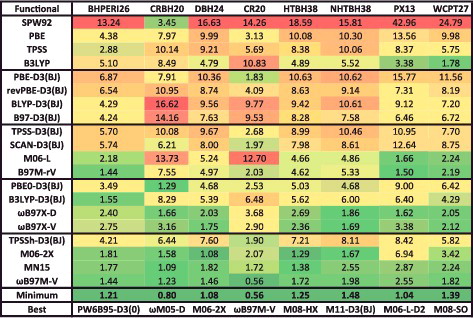
6. Effective use of density functionals

The two most important practical considerations that pertain to molecular KS-DFT calculations (apart from the choice of functional, of course) are the atomic orbital basis set [215] and the atom-centered integration grid [216]. Non-empirical density functionals should perform best at the basis set limit, while most semi-empirical density functionals are trained either at the basis set limit or close to the basis set limit. For bonded interactions, quadruple-zeta basis sets are ideal, but triple-zeta basis sets can act as substitutes for larger systems. For non-covalent interactions, reaching the basis set limit is less demanding if the Boys– Bernardi counterpoise correction scheme is used [217]. With the use of counterpoise corrections, an augmented triple-zeta basis set usually represents the CBS limit for most systems, and even some augmented double-zeta basis sets may suffice. On the other hand, if counterpoise corrections are unavailable, it is preferable to use an augmented quadruple-zeta basis set, or at the very least, a large heavily-augmented triple-zeta basis set. It is worth mentioning, however, that certain semi-empirical density functionals [218], primarily from the Truhlar group, are not compatible with counterpoise corrections and should be utilised without corrections for basis set superposition error.

Based on the extensive tests performed on the latest functional developed by the present authors (ωB97M-V), the following basis sets are recommended for DFT calculations on bonded interactions (in order of decreasing size): aug-pc-3, aug-cc-pVQZ, pc-3, def2-QZVPPD, def2-QZVPP, aug-pc-2, and pc-2. The first five are quadruple-zeta basis sets, while the latter two are triple-zeta basis sets. Of the quadruple-zeta basis sets, def2-QZVPP and pc-3 are particularly good choices as they have fewer basis functions than the augmented ones, while pc-2 is recommended from the triple-zeta basis sets as an economic choice for quick yet reasonably accurate calculations. For nonbonded interactions, if counterpoise corrections are to be neglected, then it is best to stick to an augmented, quadruple-zeta basis set, such as def2-QZVPPD, aug-pc-3, aug-cc-pVQZ, or pc-3. With the use of counterpoise corrections, several other basis sets are recommended along with the aforementioned ones, including def2-QZVPP, aug-pc-2, def2-TZVPPD, pc-2, and cc-pVQZ.

While it is beyond the scope of this paper to assess the performance of a range of functionals with a variety of basis sets, this information is available in a number of thorough studies [20,218–220]. It is noteworthy that the basis set convergence of DFT is similar to that of HF (i.e. exponential), while wave function theories exhibit significantly slower polynomial convergence. Figure 27 contains data for three of the functionals considered in this review (PBE-D3(BJ), B3LYP-D3(BJ), ωB97M-V) computed with four different basis sets: 6-31G*, def2-SVPD, def2-TZVPPD, and def2-QZVPPD, all without counterpoise corrections. This information is included primarily as a warning to users who prefer to utilise small basis sets such as 6-31G*, but additionally to explore the basis set convergence of several density functionals within a select family of basis sets. In addition, results for the ‘low-cost’ PBEh-3c method by Grimme et al. [221] are included for comparison to the 6-31G* and def2-SVPD basis set results. The PBEh-3c method was developed to be used with the very small def2-mSVP basis set. To illustrate the size of these basis sets, 6-31G*, def2-mSVP, def2-SVPD, def2-TZVPPD, and def2-QZVPPD contain 307, 307, 474, 896, and 1566 basis functions for the adenine-thymine complex, respectively.

Figure 27. RMSDs in kcal/mol for PBE-D3(BJ), B3LYP-D3(BJ), and ωB97M-V for the eight datatypes (as well as 81 equilibrium bond lengths (EBL) in Ångström and 81 equilibrium binding energies (EBE) in kcal/mol) computed with four different basis sets: 6-31G*, def2-SVPD, def2-TZVPPD, and def2-QZVPPD. Results for the ‘low-cost’ PBEh-3c method by Grimme and co-workers are given in the last row, in order to demonstrate that if modern functionals are to be used with small basis sets like 6-31G*, it is better to use a method developed for use with a small basis set.

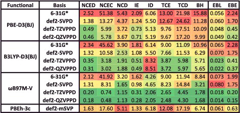
The first relevant comparison that can be made using Figure 27 is the performance of functionals near the basis set limit (def2-QZVPPD) relative to a very small basis set (6-31G*). Along with this comparison, the PBEh-3c results will be highly pertinent, as this method represents an attempt to parameterise a functional specifically for use with a small basis set. Considering first the non-covalent interactions in NCED, the performance of PBE-D3(BJ) degrades by more than a factor of 5 when transitioning from def2-QZVPPD to 6-31G*, B3LYP-D3(BJ) degrades by more than a factor of 7.5, and ωB97M-V degrades by more than a factor of 10. Clearly, these functionals are unsuitable for use with such a small basis set, and if the 6-31G* basis set must be utilised due to the size of the system, then simply using a ‘low-cost’ approach like PBEh-3c yields better results, as it has a smaller NCED RMSD than any of the three functionals in 6-31G*. This same degradation is evident for most of the other datatypes: the performance of ωB97M-V degrades by a factor of 87 for NCEC, 5.8 for IE, 3.6 for TCE, and 5.3 for BH. Despite the fact that PBEh-3c is clearly a better choice if the 6-31G* basis set must be used with these functionals, it is noteworthy that the performance of PBEh-3c is not nearly as good as any of the three functionals near the basis set limit (or even def2-SVPD in many cases).

It is also interesting to examine the convergence of these functionals toward the basis set limit within a consistent family of basis sets, namely, def2-SVPD, def2-TZVPPD, and def2-QZVPPD. Clearly, the def2-SVPD results are quite poor, for both bonded and nonbonded interactions. For instance, the NCED RMSD for ωB97M-V in def2-SVPD is more than seven times larger than the RMSD in def2-QZVPPD, while the performance for TCE across the same basis sets differs by a factor of more than 3. However, it is encouraging that the differences between the def2-TZVPPD and def2-QZVPPD results are remarkably small. For instance, the NCED RMSD of ωB97M-V is 0.20 kcal/mol in def2-TZVPPD and 0.18 kcal/mol in def2-QZVPPD. The change for thermochemistry (TCE for example) is also small (2.65 kcal/mol in def2-TZVPPD vs. 2.48 kcal/mol in def2-QZVPPD). These results indicate that a triple-zeta basis set, such as def2-TZVPPD, is perhaps sufficient for more efficient yet acceptably accurate DFT calculations. At the same time, it is important to point out that for nearly all of the datatypes, the results improve when going from def2-TZVPPD to def2-QZVPPD for all three functionals. Therefore, it is ultimately best to utilise density functionals as close to the basis set limit as possible, in order to realise their full potential.

As far as the integration grid is concerned, LSDA and GGA functionals tend to require similar integration grids and are much less sensitive to the quadrature than meta-GGA functionals. For bonded interactions, LSDA and GGA functionals can generally be used with grids such as a (50,194) grid that has 50 radial shells per atom, with 194 points per shell (or even its pruned version, SG-1). For nonbonded interactions, it is advisable to use a (75,302) grid for LSDA and GGA functionals. On the other hand, meta-GGA functionals, particularly semi-empirical ones, require at least a (75,302) grid for bonded interactions. For nonbonded interactions, the use of a (99,590) grid is advised (although some meta-GGA functionals will require even finer grids for weakly bound complexes). Recently, pruned versions of the (75,302) and (99,590) grids (SG-2 and SG-3, respectively) were published [222], which should greatly expedite calculations with functionals that require fine grids.

Comprehensive integration grid tests for density functionals are less common than basis set limit tests, but a variety of papers can be found in the literature pertaining to the grid sensitivity of certain meta-GGAs [70–72], particularly the Minnesota density functionals. However, it is not just the Minnesota functionals that are prone to grid errors. Any functional that uses the kinetic energy density as an input variable can potentially encounter similar issues. It is advisable that upon development and publication of a new density functional (especially a meta-GGA), the authors extensively test their new method to determine its behavior with respect to both the basis set and the integration grid. Unfortunately, this is not yet common practice, and such studies only exist for a few recent functionals[18–20]. However, such validation can greatly facilitate appropriate use of a functional. While a thorough investigation of the integration grid limit for the 200 functionals in this study is beyond the scope of this paper, the grid sensitivity of 20 functionals is analysed for nonbonded interactions via the NC15 data-set (Figure 28), and for bonded systems via the AlkAtom19 data-set (Figure 29). Finally, Figure 30 plots the PEC of the benzene– neon dimer for these 20 density functionals in order to visually depict the grid sensitivity of different types of functionals.

Figure 28. Mean absolute percent integration grid errors for 20 density functionals, relative to the 15 binding energies from the NC15 data-set computed with a (500,974) grid. A regularisation value of 0.01 kcal/mol is included in the denominator in order to cap excessively large percentage errors for very weakly bound systems. A value of 1% or smaller is deemed acceptable for these interactions.

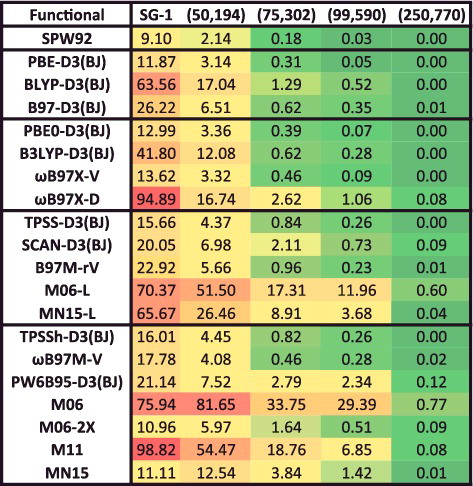
Figure 29. Root-mean-square integration grid errors in kcal/mol for 20 density functionals, relative to the 19 atomisation energies from the AlkAtom19 data-set computed with a (500,974) grid. A value of 0.05 kcal/mol or smaller is deemed acceptable for these interactions.

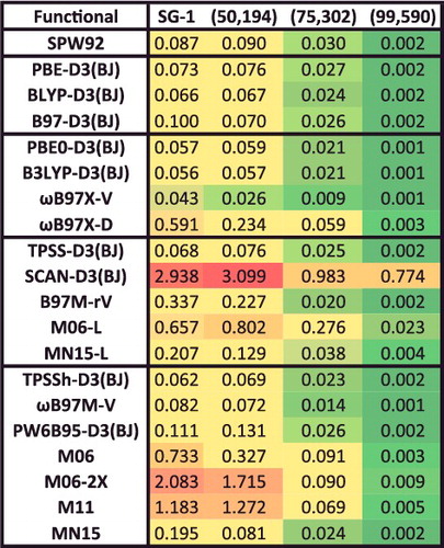
Figure 30. Benzene–neon dimer potential energy curves (PEC) computed with 20 density functionals with a (99,590) integration grid. The top subfigure shows LSDA, local GGA, and hybrid GGA functionals, and a majority of these functionals are converged with respect to the employed grid. The middle subfigure shows local meta-GGA functionals, while the bottom subfigure shows hybrid meta-GGA functionals. It is evident that the PECs of many of the meta-GGAs are sensitive to the integration grid.

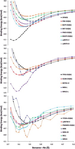
Figure 28 contains mean absolute percent integration grid errors (MAPE) for 20 density functionals, relative to the 15 binding energies from the NC15 data-set computed with a (500,974) grid. A regularisation value of 0.01 kcal/mol is included in the denominator in order to cap excessively large percentage errors for very weakly bound systems. Based on the convergence of the LSDA (SPW92), it appears that a value of under 1% is an acceptable target. Most of the local and hybrid GGA functionals are insensitive to the grid, achieving MAPEs under 1% even with a (75,302) grid. A notable exception is ωB97X-D, which has a relatively large MAPE of 2.62% with a (75,302) grid. This slow convergence could possibly be related to the fact that its power series ICFs are quartic, while the other GGA functionals have quadratic ICFs at most. Nevertheless, ωB97X-D manages to approach an MAPE of 1% with a (99,590) grid. Moving on to the meta-GGAs, the five local meta-GGAs behave very differently with respect to the grid. The non-empirical TPSS-D3(BJ) functional is only slightly more sensitive to the grid than the GGAs, still achieving an MAPE of under 1% in a (75,302) grid. Surprisingly, the semi-empirical B97M-rV functional, despite containing sixth-order terms in its ICFs, is as well-behaved as TPSS-D3(BJ). SCAN-D3(BJ), on the other hand, is 2–3 times more sensitive than TPSS-D3(BJ), while the two local Minnesota functionals, M06-L and MN15-L are most sensitive to the grid, and only achieve an MAPE of 1% with a (250,770) grid. Even with a (99,590) grid, M06-L has an MAPE of 11.96%, while MN15-L is considerably better behaved, with an MAPE of 3.68%. Finally, the hybrid meta-GGAs also display a variety of different behaviours. The only non-empirical hybrid meta-GGA functional considered is TPSSh-D3(BJ), and it behaves similarly to TPSS-D3(BJ). The semi-empirical ωB97M-V functional is even less sensitive to the grid than TPSSh-D3(BJ), which is remarkable considering the fact that it contains 12 linear parameters, and a seventh-order term in its ICF. From the remaining hybrid meta-GGAs, M06 and M11 are ill-behaved, and require a (250,770) grid to be appropriately converged with respect to the grid. MN15 vastly improves upon these two functionals, yet it still requires a (99,590) grid to meet the 1% MAPE mark. Of the four hybrid Minnesota functionals considered, M06-2X is the least sensitive to the grid.

Moving on to bonded systems, Figure 29 contains root-mean-square integration grid errors in kcal/mol for 20 density functionals, relative to the 19 atomisation energies from the AlkAtom19 data-set computed with a (500,974) grid. Before considering the different types of functionals and their grid sensitivity, it is necessary to point out the remarkable sensitivity of SCAN-D3(BJ) to the integration grid for these atomisation energies. With a (75,302) grid, it is more than 10 times more sensitive than any other functional tested. The conventional wisdom is that coarser grids can be used for thermochemistry, yet the SCAN-D3(BJ) results do not adhere to this convention. The LSDA (SPW92) has an RMSD of 0.030 kcal/mol in a (75,302) grid, and thus, a RMSD value around 0.05 kcal/mol or smaller is deemed acceptable for these atomisation energies. As with the NC15 data-set, the local and hybrid GGAs are very well-behaved, with the exception of ωB97X-D, which manages an RMSD of 0.059 kcal/mol in a (75,302) grid, which is at least a factor of 2 larger than the other GGAs. The local meta-GGAs have contrasting behaviours once again, with TPSS-D3(BJ), B97M-rV, and MN15-L being well-behaved and converged with a (75,302) grid, while M06-L requires a (99,590) grid to achieve an RMSD of under 0.05 kcal/mol. Finally, most of the hybrid meta-GGAs are relatively well behaved, and this includes TPSSh-D3(BJ), ωB97M-V, PW6B95-D3(BJ), and MN15. The other three Minnesota functionals, M06, M06-2X, and M11, are slightly more sensitive and may require a (99,590) grid, depending on the desired level of accuracy.

Figure 30 plots the PEC of the benzene-neon dimer for 20 density functionals computed with a (99,590) grid. The top subfigure plots LSDA, local GGA, and hybrid GGA density functionals, and it is evident that most of these functionals are well behaved, even for this very weak, dispersion-dominated system that is bound by about -0.5 kcal/mol. Despite being severely overbound, SPW92 is completely free of any visible oscillations. The non-empirical GGAs (PBE-D3(BJ) and PBE0-D3(BJ)) and the very lightly parameterised GGAs (BLYP-D3(BJ) and B3LYP-D3(BJ)) tend to display little to no sensitivity to the grid. Even the minimally-parameterised ωB97X-V functional, which only has six linear DFT-related parameters, is mostly free of any oscillations. The PEC for B97-D3(BJ) is only slightly more oscillatory, and it is perhaps not a coincidence that the functional has a few more linear DFT-related parameters (a total of 9). Even though ωB97X-D had a relatively large MAPE of 1.06% in a (99,590) grid for the NC15 data-set, the result for this system appears fairly well converged.

The middle subfigure plots PECs for a variety of local meta-GGAs, and there is a wide spectrum of behaviors contained in the plot. The PEC of SCAN-D3(BJ) appears to be smooth and well-behaved, while TPSS-D3(BJ) and B97M-rV display slight departures from the expected form for a PEC. M06-L is the most oscillatory of the five local meta-GGAs, and the reason for this is that M06-L makes use of VSXC-type ICFs[66], and these have been shown to lead to severe sensitivity to the grid [70,71], particularly in some of the older Minnesota functionals. VSXC-type enhancement factors are not recommended for use in future functionals, unless the functional form is sufficiently modified to reduce its grid sensitivity. Finally, MN15-L represents a recent attempt by the Truhlar group to develop a better behaved local meta-GGA. Although it exhibits much fewer oscillations than M06-L, it is still more sensitive to the grid than TPSS-D3(BJ), SCAN-D3(BJ), and B97M-rV.

The bottom subfigure contains a selection of hybrid meta-GGAs. By far the most ill-behaved functional is PW6B95-D3(BJ) by Truhlar and co-workers, as it wildly oscillates across the entire range that is plotted. This behavior is entirely due to the B95 correlation functional [71], and other functionals that utilise this correlation component are similarly ill-behaved. Furthermore, in the process of generating the data for this review, functionals that contained B95-like components were by far the most difficult to converge, and as a result, use of the B95 correlation functional is not recommended in future density functionals either (despite the fact that some recent functionals, particularly double hybrids, still utilise it [196,223]). The PEC of M06 is extremely ill-behaved, due to the use of a VSXC-type enhancement factor. While M11 and MN15 are not as sensitive as M06, they still exhibit clear oscillations. TPSSh-D3(BJ), ωB97M-V, and M06-2X, despite having some slight visible issues, are the best behaved of the hybrid meta-GGAs. Ultimately, it is the duty of the functional developers to elucidate potential issues with a new functional, and not the duty of the users to unearth shortcomings during the course of a study. While these three distinct integration grid tests are still limited in scope, they paint a picture that can be generalised to give a few broad conclusions.

• Most GGA density functionals are insensitive to the integration grid for both bonded and nonbonded interactions, and a (75,302) grid should suffice for most systems. This is supported by the fact that the NC15 integration grid MAPE of six of the seven GGAs considered is around or under 1% with this grid. Furthermore, the AlkAtom19 integration grid RMSD for the same six GGAs is under 0.03 kcal/mol with a (75,302) grid.

• GGAs are not completely exempt from integration grid errors, particularly those with higher order ICFs, such as ωB97X-D.

• meta-GGAs are far less consistent than GGAs with respect to the grid. Of the functionals tested here, TPSS-D3(BJ), B97M-rV, TPSSh-D3(BJ), and ωB97M-V are almost as well-behaved as the GGAs and a (75,302) grid may be sufficient. However, it is best to individually test the grid sensitivity of meta-GGAs, since the small selection tested here displayed widely varying behaviors.

• Any meta-GGA that utilises a B95-like or VSXC-like component should be used with extreme caution when weak interactions are being considered.

7. Case studies

In order to demonstrate the utility of the best density functionals considered in this work, results for three case studies will be discussed. However, instead of presenting data for the 20 featured functionals, the 13 functionals that will be ultimately recommended in the concluding comments will be utilised. These functionals are B97-D3(0), revPBE-D3(0), and BLYP-D3(0) from the local GGAs, B97M-rV, MS1-D3(0), and M06-L-D3(0) from the local meta-GGAs, ωB97X-V, ωB97X-D3, and ωB97X-D from the hybrid GGAs, and ωB97M-V, ωM05-D, M06-2X-D3(0), and MN15 from the hybrid meta-GGAs. The first case study is representative of transition metal chemistry and considers a model system for a second generation Grubbs catalyst often used in olefin metathesis. The original work is from Zhao and Truhlar [224], and the reference values have recently been refined by Kesharwani and Martin [225]. The second case study is representative of biological chemistry and hails from a very recent paper by Hobza and co-workers on protein–DNA interactions in biological processes. Complexes involving amino acids and nucleotides were extracted from the PDB, and following an extensive refinement of the initial structures, CCSD(T)/CBS interaction energies were computed for 12 representative complexes. Finally, the last case study involves a total of 2510 water dimer configurations extracted from a molecular dynamics simulation [226], with highly accurate reference values recomputed by Sherrill et al. [117]. The centre-of-mass separation of the dimers ranges from 2.12 to 7.97 Å (equilibrium is around 2.95 Å). Henceforth, these three case studies are referred to as Grubbs, PDB12, and Water2510, respectively. Visualisations of the systems contained in the case studies are shown in Figure 31, with the top panel corresponding to the Grubbs case study, the middle panel corresponding to the PDB12 case study, and the bottom panel corresponding to the Water2510 case study.

Figure 31. Visual representations of the three case studies considered in Section 7. The top panel corresponds to the Grubbs case study, the middle panel corresponds to the PDB12 case study, and the bottom panel corresponds to the Water2510 case study.

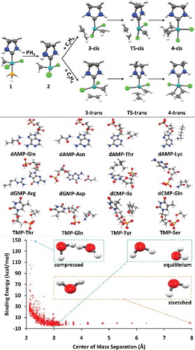
7.1. Grubbs catalyst model system

While there is an abundance of highly accurate benchmark data available for molecules composed of the main-group elements, reliable reference values for transition metal systems are far less common. Therefore, it is standard practice to utilise experimental values with the proper corrections. A recent study by Truhlar et al. [227] concluded that CCSD(T) should not be used as a reference to validate density functionals, which complicates the proper benchmarking of density functionals for transition metal chemistry. Very recently, however, two studies [228,229] demonstrated that CCSD(T) can be reliably used for the prediction of transition metal bond dissociation energies. Nevertheless, it is important to verify that the best functionals resulting from this study are capable of handling transition metals with reasonable accuracy, since the database utilised thus far is entirely composed of main-group elements. The Grubbs case study consists of stationary points in the catalytic cycle of the Grubbs II catalyst and contains seven data points in total (top panel of Figure 31). The revised CCSD(T*)-F12b/def2-AQZVPP reference values from Martin and Kesharwani are employed [225], specifically the ones that correlate the (4s,4p) subvalence orbitals of the Ruthenium atom, and the energies are taken relative to 2 + C₂H₄. For the Grubbs data-set only, the def2-TZVP basis set is used instead of def2-QZVPPD.

The 13 functionals considered have RMSDs ranging from 1.21 kcal/mol to 9.48 kcal/mol, shown in Figure 32. The three local GGAs perform poorly, with BLYP-D3(0) and B97-D3(0) having RMSDs above 9 kcal/mol, while revPBE-D3(0) manages an RMSD of 4.38 kcal/mol. The local meta-GGAs consistently improve upon the local GGAs, with MS1-D3(0) affording the best overall RMSD of 1.21 kcal/mol. In comparison, B97M-rV performs about 2 times worse than MS1-D3(0), while M06-L-D3(0) performs about 3 times worse. From the hybrid GGAs, ωB97X-D and ωB97X-D3 manage RMSDs slightly in excess of 3 kcal/mol, while ωB97X-V comes in at 2.27 kcal/mol. Finally, the hybrid meta-GGAs are interesting since the design principles of MN15 intended to maintain the good performance of M06-2X for main-group thermochemistry, while improving performance for transition metals. Indeed, MN15 performs about 2 times better than M06-2X-D3(0). However, despite the fact that MN15 was trained on transition metals and ωB97M-V was neither trained nor tested on them, the latter functional manages to outperform MN15 by about 30%. Overall, only 5 of the 13 functionals manage RMSDs under 3 kcal/mol: MS1-D3(0), ωB97M-V, ωB97X-V, MN15, and B97M-rV.

Figure 32. Relative energies in kcal/mol for the Grubbs case study for 13 density functionals. Mean signed errors (MSE) and root-mean-square deviations (RMSD) are shown at the bottom. The top panel of Figure 31 contains more information regarding these interactions.

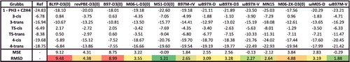
7.2. Protein–DNA interactions from the PDB

Benchmark studies involving biologically relevant complexes exhibiting non-covalent interactions are of vital importance to the development of force fields and other efficient computational methods. The PDB12 case study contains 12 protein–DNA complexes from a very recent study by Hobza et al. [230]. Since the complexes are rather large (58 atoms at most), the reference values are not computed at the same level of quality as popular data-sets like S22 and S66. The conventional CCSD(T)/CBS composite scheme is utilised, with the HF energy calculated with the aug-cc-pVQZ basis set, the MP2 contribution computed with MP2-F12/cc-pVDZ-F12, and the CCSD(T) Δ-correction performed with the modified 6-31G**(0.25,0.15) basis set. Since counterpoise corrections are employed, these reference values approach the basis set limit from above (i.e. they are most likely slightly underbound). It is also important to note that 10 of the 12 complexes in PDB12 are negatively charged. The abbreviations for the monomers are: dAMP - deoxyadenosine monophosphate, dGMP - deoxyguanosine monophosphate, dCMP - deoxycytidine monophosphate, TMP - thymidine monophosphate, Gln - glutamine, Asn - aspargine, Thr - threonine, Lys - lysine, Arg - arginine, Asp - aspartic acid, Ile - isoleucine, Gln - glutamine, Tyr - tyrosine, and Ser - serine.

The binding energies and relevant statistics for the PDB12 case study can be found in Figure 33, while the complexes are shown in the middle panel of Figure 31. Most of the local functionals perform poorly for these 12 interactions, with RMSDs in the vicinity of 1 kcal/mol. The only local functional that performs reasonably well is B97M-rV, managing an RMSD of 0.56 kcal/mol. The hybrid functionals perform significantly better than the majority of the local functionals, with two exceptions: MN15, with an RMSD of 1.17 kcal/mol, performs the worst from among all 13 functionals, while ωM05-D performs comparably to the local GGAs, with an RMSD of 0.94 kcal/mol. Consistent with the NCED and NCEC results from Section 5.2, the best-performing methods are ωB97M-V and ωB97X-V, with RMSDs of 0.34 kcal/mol. It is remarkable that these functionals predict strikingly similar binding energies for all 12 complexes. Furthermore, the slightly negative MSEs are also encouraging, since reference values that are closer to the basis set limit should be systematically more bound, potentially reducing the MSEs and RMSDs of these two functionals (and other functionals with negative MSEs). The rest of the hybrids perform comparably to the best local functional, with RMSDs between 0.5 and 0.6 kcal/mol.

Figure 33. Binding energies in kcal/mol for the PDB12 case study for 13 density functionals. Mean signed errors (MSE) and root-mean-square deviations (RMSD) in kcal/mol are shown at the bottom. The middle panel of Figure 31 contains more information regarding these interactions.

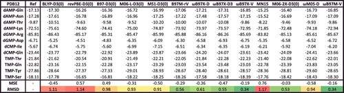
7.3. Water dimer potential energy surface

Force fields that can accurately capture the intricacies of water molecules interacting with themselves or their environment are valuable tools for the determination of properties of liquid water and solvation effects, respectively. However, in order to determine the parameters of a force field, accurate training data is of vital importance. While CCSD(T)/CBS is the ideal model chemistry for generating such data, density functional calculations are highly desirable as an alternative since they can be applied to larger system sizes without hitting a computational bottleneck. Additionally, it is important to

sample all parts of the potential energy surface of interacting water molecules. The Water2510 data-set is interesting in this regard, as it contains CCSD(T)/CBS interaction energies for 2510 water dimers exhibiting vastly different orientations and separations, and can be used to identify density functionals that can be potentially used to study water.

Since the data-set is vast, individual binding energies are not provided for Water2510. Instead, Figure 34 contains several relevant statistical measures for the 13 tested density functionals. MSEs and RMSDs are reported for the full set, and also decomposed into positive binding energies (E ≥ 0) and negative binding energies (E < 0). The bottom panel of Figure 31 plots the binding energy of each water dimer from Water2510 against the corresponding center of mass separation. It is evident that highly compressed, highly stretched, and near equilibrium configurations are present in the data-set. Considering first the overall RMSDs, the performance of ωB97M-V is remarkable, as it manages an RMSD of only 0.16 kcal/mol. The next best functional, M06-2X-D3(0), performs two times worse, with an RMSD of 0.29 kcal/mol. In accordance with Jacob's Ladder, the local GGAs perform worst, with BLYP-D3(0) managing an RMSD of 0.63 kcal/mol, significantly outperforming the other two functionals in its class. The local meta-GGAs soundly improve upon the local GGAs, with M06-L-D3(0) affording an overall RMSD of 0.44 kcal/mol, and B97M-rV performing about 20% better with an RMSD of 0.35 kcal/mol. While none of the hybrids manage to come close to the performance of ωB97M-V, the RMSD of ωB97X-V is nearly identical to that of M06-2X-D3(0).

Figure 34. Mean signed errors (MSE) and root-mean-square deviations (RMSD) in kcal/mol for the Water2510 case study for 13 density functionals. The statistics are further separated into unbound configurations (E ≥ 0) and bound configurations (E < 0). The bottom panel of Figure 31 contains more information regarding these interactions.

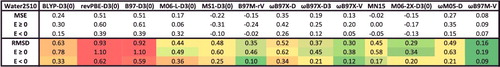
The partitioning of the statistics into the two distinct energetic classes clearly demonstrates that most of the errors are coming from the highly compressed (repulsive) region (E ≥ 0). For these configurations, the best-performing functional, ωB97M-V, has an RMSD of 0.19 kcal/mol, while its RMSD for the bound configurations (E < 0) is more than a factor of 2 smaller, at 0.09 kcal/mol. Considering only the bound dimers, the three combinatorially optimised functionals that employ the VV10 NLC functional perform remarkably well, with RMSDs of 0.09 kcal/mol (ωB97M-V), 0.10 kcal/mol (B97M-rV), and 0.12 kcal/mol (ωB97X-V). In contrast, ωB97X-D performs almost four times worse than ωB97M-V, while the rest of the hybrids manage RMSDs between 0.17 and 0.21 kcal/mol. Overall, ωB97M-V presents itself as a very promising choice for sampling the entire potential energy surface of water molecules, as its performance for Water2510 complements its accuracy for the water cluster data-sets already considered in the primary database.

8. Summary and conclusions

8.1. Summary

A vast amount of computational and human effort was devoted to making this review of density functionals as exhaustive as possible. With data for 200 functionals across 84 data-sets containing 4986 data points that required 5931 single-point calculations per functional, this amounts to more than a million single-point calculations near the basis set and integration grid limit for systems as large as a water 20-mer. For comparison, a recent study [231] with a similar goal benchmarked 77 density functionals across 384 data points, requiring 30 times less data. Furthermore, since a number of the functionals in this review are relatively new to the DFT literature, the routines for these functionals were specifically added into Q-Chem for this study. Some of these newer functionals include MS0, MS1, MS2, MS2h, MVS, MVSh, SCAN, SCAN0, BLOC, TM, N12, N12-SX, MN12-L, MN12-SX, GAM, MN15, MN15-L, oTPSS, mBEEF, and rVV10, and are being extensively benchmarked here for the first time. As a result, it would be unfortunate if at least some data for all 200 functionals did not appear in the main body of the review. Therefore, RMSDs for all 200 functionals for the eight datatypes are shown in Figures 35–42, and the results for the four most relevant datatypes will be discussed (NCED, IE, TCE, and BH in Figures 35, 38, 40, and 42, respectively). While the tables are rather large and data oriented, a careful study can reveal a great deal of information about the performance of any given functional relative to the state-of-the-art, especially since most functionals currently in use have been included in the list of 200.

Figure 35. Sorted NCED RMSDs in kcal/mol for all 200 benchmarked density functionals. NCED contains 1744 non-covalent dimer interactions.

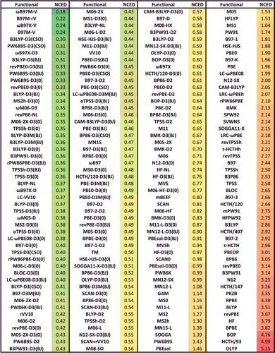
Figure 36. Sorted NCEC RMSDs in kcal/mol for all 200 benchmarked density functionals. NCEC contains 243 non-covalent cluster interactions.

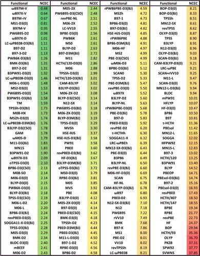
Figure 37. Sorted NCD RMSDs in kcal/mol for all 200 benchmarked density functionals. NCD contains 91 difficult non-covalent dimer interactions.

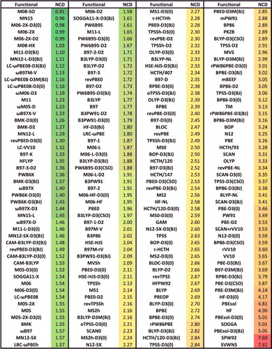
Figure 38. Sorted IE RMSDs in kcal/mol for all 200 benchmarked density functionals. IE contains 755 isomerisation energies.

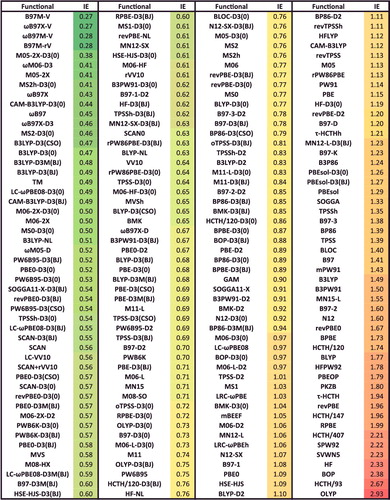
Figure 39. Sorted ID RMSDs in kcal/mol for all 200 benchmarked density functionals. ID contains 155 difficult isomerisation energies.

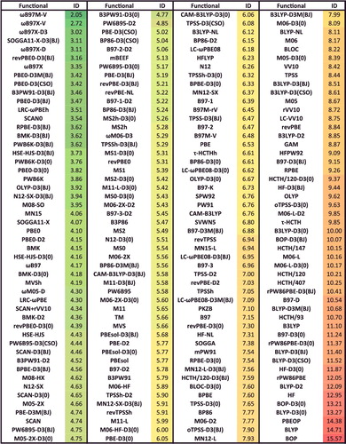
Figure 40. Sorted TCE RMSDs in kcal/mol for all 200 benchmarked density functionals. TCE contains 947 thermochemistry data points.

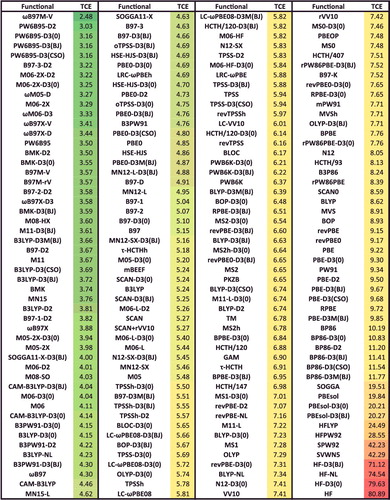
Figure 41. Sorted TCD RMSDs in kcal/mol for all 200 benchmarked density functionals. TCD contains 258 difficult thermochemistry data points.

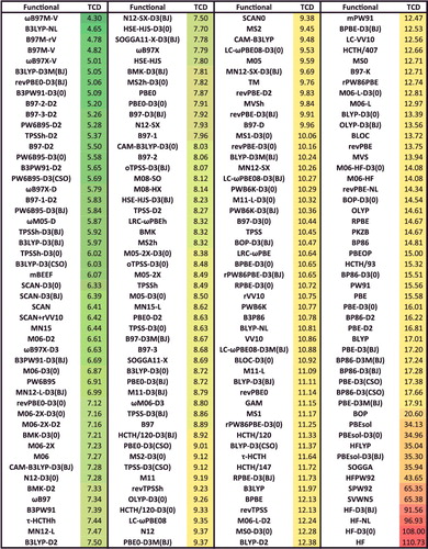
Figure 42. Sorted BH RMSDs in kcal/mol for all 200 benchmarked density functionals. BH contains 206 barrier heights.

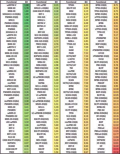
Figure 35 deals with the NCED datatype. It is remarkable that the first column of 50 functionals contains only dispersion-corrected functionals, with the RMSD range starting at 0.18 kcal/mol with ωB97M-V and ending with B3PW91-D3(BJ) at 0.43 kcal/mol. Thus, functionals that do not utilise dispersion corrections are at least 2.4 times worse than the state-of-the-art for conventional non-covalent dimers. It is interesting to look at the functionals that occupy the fourth column, as they represent the 50 worst functionals for NCED. In last place is the OLYP functional, a combination of the OPTX exchange functional and the LYP correlation functional. HF is fifth worst, with an RMSD of 3.79 kcal/mol, and it is clear that most of the functionals in this column were developed before the emphasis of DFT turned from thermochemistry to non-covalent interactions. However, some modern (post-2010) functionals are ranked in the bottom 50, including N12, BLOC, SOGGA11-X, N12-SX, and MS1. While BLOC and MS1 are non-empirical functionals that certainly require dispersion corrections (just like TPSS needs a dispersion correction), it is surprising that three functionals trained on non-covalent interactions (N12, SOGGA11-X, and N12-SX) make it into this list. Although HF is fifth worst, the addition of the D3(BJ) dispersion tail improves its performance by a factor of 5, and it performs comparably to functionals such as M06 and SCAN, despite known errors in long-range electrostatic interactions[232].

Figure 38 ranks the RMSDs of all 200 functionals for the IE datatype. The functional ranking for this category is contradictory to Jacob's Ladder, with the best performer being a local meta-GGA with the VV10 NLC functional. Among the 50 worst functionals, one can find local GGAs (e.g. OLYP), hybrid GGAs (e.g. B3PW91), local meta-GGAs (e.g. τ-HCTH), and hybrid meta-GGAs (e.g. TPSSh). Besides the top performer (B97M-V) and its close relative (B97M-rV, which ranks fourth), many of the best functionals are hybrids. However, several other local functionals appear in the top 50, including MS2-D3(0), TM, and MS0-D3(0). It is also interesting to note that most of the functionals in the last column are non-dispersion-corrected functionals, indicating that dispersion corrections are important for the prediction of accurate relative energies. Only a few dispersion-corrected functionals make it into the bottom 50 for IE: PBEsol-D3(BJ), PBEsol-D3(0), MN12-L-D3(BJ), B97-D, revPBE-D2, HF-D3(0), and BP86-D2. However, comparing the RMSDs of HF (2.33 kcal/mol) and HF-D3(0) (1.19 kcal/mol) clearly indicates that the dispersion correction is helpful to a certain extent. Furthermore, while it appears that dispersion corrections are useful for these isomerisation energies, a handful of non-dispersion-corrected functionals rank in the top 50, including M05-2X, ωB97X, ωB97, TM, M06-2X, SCAN, MVS, and M08-HX. However, even the best non-dispersion-corrected functional, M05-2X, performs about 50% worse than the best overall.

The ranked RMSDs in Figure 40 are associated with the TCE datatype. Starting in reverse order, the value of DFT is immediately clear because the worst performer is HF, with an RMSD of 80.89 kcal/mol. Comparing the best and the worst demonstrates the incredible progress made by density functionals in the past several decades, as ωB97M-V is more than 30 times better than HF. Not surprisingly, the worst actual density functional is SVWN5, an LSDA functional, with an RMSD of 42.29 kcal/mol. While the worst density functional improves upon HF by a factor of 2, the state-of-the-art is capable of performing a further 20 times better. With the exception of a few outliers, the ranking of functionals in Figure 40 adheres to the ordering of Jacob's Ladder, as HF is surpassed by the LSDA, which is then surpassed by the GGA functionals that were made for extended systems (PBEsol and SOGGA). These are in turn surpassed by the GGAs that are popular for molecular applications, such as BP86, PBE, revPBE, and BLYP. Oddly, a few outliers are found in the last column, such as revPBE0 (a hybrid GGA), MVS (a local meta-GGA), SCAN0 (a hybrid meta-GGA), B3P86 (a hybrid GGA), MVSh (a hybrid meta-GGA), revPBE0-D3(BJ) (a hybrid GGA), B97-K (a hybrid GGA), as well as MS0 and its dispersion-corrected counterpart (local meta-GGAs). Skipping over to the top 50, most of the best functionals are hybrid meta-GGAs, although the hybrid GGA B97-3-D2 does manage to place sixth overall. The next best hybrid GGAs rank 12th and 13th, with RMSDs that are nearly 1 kcal/mol larger than the best possible. Surprisingly, three local functionals also appear in the top 50, namely B97M-V, B97M-rV, and MN15-L, with RMSDs of 3.57, 3.57, and 4.62 kcal/mol, respectively. However, their performance is still more than 1 kcal/mol worse than the state-of-the-art (although comparable to hybrid GGAs).

Finally, Figure 42 deals with the BH datatype. Not surprisingly, the worst performers are the two LSDA functionals and HF, while the best performers are either hybrid meta-GGAs, or hybrid GGAs with large fractions of exact exchange. An example of the latter is SOGGA11-X-D3(BJ) (40.15% global exact exchange), which impressively ranks fourth, with an RMSD of 1.89 kcal/mol. It is slightly worse than the two best Minnesota functionals for BH (M08-SO and M08-HX with RMSDs of 1.78 and 1.80 kcal/mol, respectively), and only about 10% worse than the first place functional, ωB97M-V. Other examples of successful hybrid GGAs are the range-separated hybrid GGAs, ωB97X-D3 and ωB97X-D, with RMSDs around 2.3 kcal/mol. While the smallest RMSD for BH is 1.68 kcal/mol and due to a hybrid meta-GGA, the smallest RMSD for a local functional is 4.16 kcal/mol (MN12-L-D3(BJ)), followed by MN12-L itself (4.29 kcal/mol) and then B97M-V (4.35 kcal/mol). Thus, these results make it sufficiently clear that local functionals simply cannot compete with hybrids for barrier heights. Most of the functionals in the fourth column (besides HF and the LSDA functionals) are local GGAs, with the exception of a few dispersion-corrected TPSS-based functionals.

8.2. Recommendations

In order to help conclude this comprehensive benchmark, Figure 43 summarises the main points by presenting the best of the 200 functionals, listing the top three functionals by type (local GGA, local meta-GGA, hybrid GGA, hybrid meta-GGA) for each datatype, as well as the top five functionals overall. The values to the right of the functional name represent the average rank of the functional across the data-sets in the specific datatype, while for the last row, the value is the average of the eight datatype averages from the preceding rows. The colour-coding extends only across the functionals in a specific row (i.e. NCED, NCEC, etc.). Furthermore, functionals that are close to identical (i.e. they differ due to their dispersion component) are only listed once. For example, within the NCED datatype and the local meta-GGA functional type, B97M-rV has a rank value of 9 and B97M-V has a rank value of 11, but since they only differ by their dispersion component, only the best version (B97M-rV) is allowed into the table. Another occurrence of this is with the best overall local GGA: B97-D3(0) has rank value of 98 and B97-D3(BJ) has a rank value of 101, but only the former is listed.

Figure 43. Average rankings for the best of the 200 functionals studied in this review. The functionals are ranked for each of the 82 data-sets that correspond to the eight datatypes, the rankings are averaged by datatype, and the functionals are partitioned by type (local/hybrid and GGA/mGGA). The three functionals with the best (smallest) rank populate the first eight rows of this table, and the last ‘Overall’ row is an average over the eight average datatype ranks. Functionals that differ only in their dispersion component are only listed once by selecting the best performer.

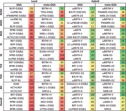
An interesting consequence of the format of Figure 43 is that the functionals obey the ordering of Jacob's Ladder (going from left to right across the nine primary rows), with the local GGAs having mostly red values, the local meta-GGAs having a mixture of colours (red for the categories that are sensitive to exact exchange and green or yellow for the others), and the hybrids generally performing well with mostly green and a few yellow values. Since the bulk of the information contained in this table has already been discussed, it is presented to aid readers in identifying either specific functionals for specific purposes (e.g. the best local GGA for thermochemistry), or for identifying the best functional overall from a certain class, regardless of the application (e.g. the best hybrid GGA overall). This table will be used to make the final recommendations pertaining to functional selection:

• Local GGA functionals: A total of 61 local GGA functionals were benchmarked in this review. For non-covalent interactions, BLYP-D3(BJ) is highly recommended, particularly for dimers and small clusters, as its performance is comparable to popular dispersion-corrected hybrids such as B3LYP-D3(BJ) and revPBE0-D3(BJ). B97-D3(0) and its two cousins, B97-D3(BJ) and B97-D3M(BJ), are recommended as the default choices from this class, especially if the particular chemical application does not conform to a specific datatype. Furthermore, revPBE-D3(0) and BLYP-D3(0) (along with their D3(BJ) and D3M(BJ) variants) are solid choices from the local GGAs. If available, dispersion corrections must be utilised with local GGA functionals, since they are incapable of treating non-covalent interactions on their own.

• Local meta-GGA Functionals: From the 35 local meta-GGA functionals benchmarked in this review, B97M-rV (or B97M-V), MS1-D3(0) (or MS2-D3(0)), and M06-L-D3(0) are the most reliable choices. B97M-rV ranks nearly a factor of 2 higher than the others, but if the rVV10 (or VV10) NLC functional is unavailable, the others should serve as good alternatives. For standard non-covalent interactions and isomerisation energies, as well as most bonded interactions, B97M-rV and B97M-V are excellent choices and can approach the performance of many standard hybrids. Furthermore, B97M-rV and B97M-V, as well as the newer Minnesota functionals (MN12-L and MN15-L) can be used for kinetics if exact exchange is unavailable.

• Hybrid GGA functionals: Overall, 53 hybrid GGA functionals were included in this review. The dispersion-corrected, range-separated hybrid functionals from the ωB97 family are prime choices, namely ωB97X-V, ωB97X-D3, and ωB97X-D, and are recommended as the default choices from this class. For non-covalent interactions and isomerisation energies, ωB97X-V is clearly superior to the other two, while all three are good for bonded interactions and barrier heights. B3LYP-D3(CSO) and B3LYP-D3(BJ) perform very well for non-covalent interactions, while a great hybrid GGA specifically for BH is SOGGA11-X-D3(BJ).

• Hybrid meta-GGA functionals: In total, 44 hybrid meta-GGA functionals were considered in this review. Overall, ωB97M-V presents itself as one of the best Rung 1–4 functionals yet developed, and ranks more than a factor of 3 better than the next best hybrid meta-GGA. While the PW6B95 functional has been recommended in previous studies [233], it is not recommended here due to its convergence issues and abnormal sensitivity to the integration grid for weak interactions. ωM05-D, M06-2X-D3(0), and MN15 are suitable alternatives that are relatively well behaved. ωB97M-V is recommended for nearly all interaction types considered, perhaps with the exception of systems severely plagued by self-interaction (e.g. the TA13 data-set in NCD). For such cases, the Minnesota functionals with high fractions of exact exchange (e.g. M06-2X or MN15) are recommended. Furthermore, the 2008 Minnesota functionals (M08-HX and M08-SO) are both very good choices for BH.

• With regards to semi-empirical functional development, the combinatorial approach is highly recommended, as it has produced three minimally-parameterised functionals that comfortably outperform more parameterised functionals within their class. For instance, B97M-rV has only 12 parameters yet an overall rank of 45, while MN15-L has 58 parameters and an overall rank of 110. In addition, ωB97M-V has only 12 parameters and an overall rank of 12, while MN15 has 59 parameters and an overall rank of 47. The combinatorial approach is particularly helpful for developing functionals within the meta-GGA parameter space.

• Finally, if only one functional is to be recommended, ωB97M-V is clearly the best choice from the 200 functionals evaluated here. And if the inclusion of exact exchange is unfeasible, then B97M-rV is the leading functional. It should be noted that the extension of these conclusions to other systems, particularly solid state and liquid state systems, as well as other types of properties such as excited states and magnetic fields (discussed separately below), remains a topic for future investigation. Additionally, it should be noted that no existing density functional on Rungs 1–4 is really adequate for problems in the ‘difficult’ categories, where significant self-interaction/delocalisation errors and/or strong correlation effects are in play.

8.3. Outlook and remaining issues

This review has covered many of the issues associated with assessing the performance of density functionals for calculating chemically relevant energy differences on the ground state potential energy surface. In this final subsection, it is useful to mention briefly some of the performance issues that have not been covered. For initial perspective, note that it is a truism (and supported by the data presented already) that no practical present-day density functional is universally accurate. Rather, density functionals that lack universal accuracy are of practical value because they are computationally efficient and because most chemistry is easy for DFT, at least in the sense that numerical errors are generally acceptable with a variety of functionals. The main limitations of the functionals discussed have been the treatment of nonlocal exchange and correlation.

Errors in exchange give rise to the delocalisation error associated with SIE. The difficult non-covalent interactions (NCD) category and barrier heights (BH) category, and to some extent the difficult isomerisation energies (ID), primarily reflect this issue. Higher fractions of exact exchange reduce SIE, and therefore the best functionals for SIE-sensitive problems are global hybrids or range-separated hybrids with significant fractions of exact exchange. Some examples are in order. SIE manifests in radical-neutral complexes[144] because the odd electron delocalises too much. SIE is also significant in ionisation energies in large molecules, because the hole will typically delocalise excessively [234,235]. Mixed valence systems such as metal oxides are likewise SIE-sensitive because this leads to insufficient ionic character[236]. It is quite useful to have a general idea (based on these and other examples) of when SIE may manifest itself as large errors in DFT calculations.

Since increasingly high fractions of exact exchange reduce SIE, it is quite common to resort to wave-function based methods to reliably treat SIE-sensitive problems. Within DFT, it is also useful to use functionals from Rung 5, which have not been assessed here. Rung 5 functionals, which are often called double hybrids [132], use wave function expressions for electron correlation (typically either from second-order perturbation theory (PT2) or the random phase approximation (RPA)) in addition to wave function exchange. Such functionals often have much higher fractions of exact exchange, and therefore lower SIE. It is desirable to extend the combinatorial design approach discussed here to the development of PT2 and/or RPA-based Rung 5 density functionals, and an effort in this direction is underway. As an alternative, there are also on-going efforts to develop new descriptors [237–239] that can enable the development of functionals with lower SIE, as well as long-standing self-interaction corrections[22,240,241].

Nonlocal correlation effects beyond dispersion interactions can arise from the presence of strong electron correlation, meaning that there is more than one (and sometimes very many) determinants that contribute to the electronic wave function in an essential way. Since KS-DFT uses a single determinant, such multi-configurational effects cannot readily be captured using the functionals discussed here. The relatively poor performance of the tested functionals for the difficult thermochemistry (TCD) datatype reflects this issue, in addition to the role of some SIE. There is effort to develop density functionals that can better describe strong correlation[126–128], but such methods do not yet appear to be ready for routine applications. There are also on-going efforts to replace the single Kohn–Sham reference by a multi-configurational wave function[242]. In principle, such methods belong to Rung 5 of Jacob's Ladder, although the PT2 and RPA methods discussed above do not address the strong correlation issue. Furthermore, multi-configurational DFT methods face some of the definitional ambiguities and complexities that confront efforts to generalise single-determinant-based wave function theories to multi-configurational references.

Another area that this review has only briefly and incompletely touched is the question of molecular properties. The assessment reported above included equilibrium geometries, which are a first-order molecular property. Second-order properties such as vibrational frequencies are known to be quite well described by density functionals, while electric polarisabilities can be susceptible to SIE. Magnetic properties, such as the chemical shifts that govern NMR spectroscopy, are an interesting area where DFT has been widely applied despite significant formal limitations [243–245]. The Hohenberg– Kohn theorem in its standard form does not hold in magnetic fields, and there is either a different functional for each field strength [246] (BDFT), or the functional must additionally have current density dependence [247,248]. The development of suitable current-density-dependent functionals is at a very early stage[249], and most studies of chemical shifts simply use conventional functionals (with reasonable success [250]).

This review has concentrated entirely on the electronic ground state. The framework of time-dependent density functional theory [251] (TDDFT) allows KS-DFT to be used for calculating electronic excited states, as well as responses to time-dependent perturbations. An additional approximation, the so-called adiabatic approximation, is required to employ ground state functionals for TDDFT calculations of excited states. This is a major area, where quite a number of excellent reviews are already available [252–254]. In brief, valence excitations are often quite well-described by TDDFT, while charge-transfer and Rydberg excited states are subject to SIE, which can be reduced by range-separated hybrids, particularly with the aid of problem-specific tuning of the range-separation parameter [255]. With respect to functional development, it seems desirable to not include TDDFT calculations in training data because of the additional uncontrolled effect of the adiabatic approximation. An alternative to TDDFT is the use of constrained DFT [256] (CDFT) to obtain limited excited state information from ground state calculations with real-space constraints to force charge transfer. CDFT calculations avoid the adiabatic approximation and thus more directly reflect the strengths (and weaknesses) of the functionals used.

In conclusion, striking progress has been made in the development of density functionals over the past several decades, and the rate of progress has not slowed down in recent years. Indeed, the introduction of dispersion corrections about a dozen years ago, and the subsequent development of van der Waals density functionals, has transformed the treatment of nonbonded interactions, as evidenced by the fact that nearly all functionals recommended in this study are dispersion-corrected. Very recently, the combinatorial functional design approach developed by the present authors has enabled substantial advances in the accuracy of calculations at Rung 3 and Rung 4 of Jacob's Ladder. These conclusions, as well as the specific recommendations, should help clarify the fact that current research on developing density functionals can appear somewhat chaotic at times because of the wealth of new functional designs that are continuously appearing. The limitations and challenges mentioned in this final subsection indicate that there is still plenty of opportunity for further innovation in the future.

Acknowledgments

This research was supported by the Director, Office of Science, Office of Basic Energy Sciences, of the U.S. Department of Energy under Contract No. DE-AC02-05CH11231, with additional support from a subcontract from MURI Grant W911NF-14-1-0359. The authors are greatly indebted to Jonathon Witte for independently validating the database used in the review. The authors thank Susi Lehtola for carefully proofreading the manuscript and providing helpful comments. The authors also thank Yuezhi Mao and Joonho Lee for helpful comments and discussions.

Disclosure statement

No potential conflict of interest was reported by the authors

Additional information

Funding

Basic Energy Sciences [grant number DE-AC02- 05CH11231]; MURI [grant number W911NF-14-1-0359]

References

- P. Hohenberg and W. Kohn, Phys. Rev. 136, B864 (1964).
- L.H. Thomas, Math. Proc. Cambridge Philos. Soc. 23, 542 (1927).
- W. Kohn and L.J. Sham, Phys. Rev. 140, A1133 (1965).
- Y.A. Wang, N. Govind, and E.A. Carter, Phys. Rev. B 60, 16350 (1999).
- B. Zhou, V.L. Ligneres, and E.A. Carter, J Chem. Phys. 122, 044103 (2005).
- J. Xia, C. Huang, I. Shin, and E.A. Carter, J. Chem. Phys. 136, 084102 (2012).
- J.P. Perdew, K. Burke, and M. Ernzerhof, Phys. Rev. Lett. 77, 3865 (1996).
- J. Tao, J.P. Perdew, V.N. Staroverov, and G.E. Scuseria, Phys. Rev. Lett. 91, 146401 (2003).
- A.D. Becke, J. Chem. Phys. 98, 5648 (1993).
- A.D. Becke, J. Chem. Phys. 107, 8554 (1997).
- K. Raghavachari, G.W. Trucks, J.A. Pople, and M. Head-Gordon, Chem. Phys. Lett. 157, 479 (1989).
- R.J. Bartlett and M. Musiał, Rev. Mod. Phys. 79, 291 (2007).
- J.D. Chai and M. Head-Gordon, J. Chem. Phys. 128, 084106 (2008).
- J. Sun, R. Haunschild, B. Xiao, I.W. Bulik, G.E. Scuseria, and J.P. Perdew, The J. Chem. Phys. 138, 044113 (2013).
- J.P. Perdew, A. Ruzsinszky, J. Tao, V.N. Staroverov, G.E. Scuseria, and G.I. Csonka, J. Chem. Phys. 123, 062201 (2005).
- M.G. Medvedev, I.S. Bushmarinov, J. Sun, J.P. Perdew, and K.A. Lyssenko, Sci. 355, 49 (2017).
- N. Mardirossian and M. Head-Gordon, J. Chem. Phys. 140, 18A527 (2014).
- N. Mardirossian and M. Head-Gordon, Phys. Chem. Chem. Phys. 16, 9904 (2014).
- N. Mardirossian and M. Head-Gordon, J. Chem. Phys. 142, 074111 (2015).
- N. Mardirossian and M. Head-Gordon, J. Chem. Phys. 144, 214110 (2016).
- S.H. Vosko, L. Wilk, and M. Nusair, Can. J. Phys. 58, 1200 (1980).
- J.P. Perdew and A. Zunger, Phys. Rev. B 23, 5048 (1981).
- J.P. Perdew and Y. Wang, Phys. Rev. B 45, 13244 (1992).
- D.M. Ceperley and B.J. Alder, Phys. Rev. Lett. 45, 566 (1980).
- F. Herman, J.P. Van Dyke, and I.B. Ortenburger, Phys. Rev. Lett. 22, 807 (1969).
- F. Herman, I.B. Ortenburger, and J.P. Van Dyke, Int. J. Quant. Chem. 4, 827 (1969).
- K. Schwarz, Chem. Phys. 7, 94 (1975).
- A.D. Becke, J. Chem. Phys. 84, 4524 (1986).
- A.D. Becke, Phys. Rev. A 38, 3098 (1988).
- J.P. Perdew, J.A. Chevary, S.H. Vosko, K.A. Jackson, M.R. Pederson, D.J. Singh, and C. Fiolhais, Phys. Rev. B 46, 6671 (1992).
- Y. Zhang and W. Yang, Phys. Rev. Lett. 80, 890 (1998).
- B. Hammer, L.B. Hansen, and J.K. Nørskov, Phys. Rev. B 59, 7413 (1999).
- J.P. Perdew, A. Ruzsinszky, G.I. Csonka, O.A. Vydrov, G.E. Scuseria, L.A. Constantin, X. Zhou, and K. Burke, Phys. Rev. Lett. 100, 136406 (2008).
- J.P. Perdew, Phys. Rev. B 33, 8822 (1986).
- C. Lee, W. Yang, and R.G. Parr, Phys. Rev. B 37, 785 (1988).
- F.A. Hamprecht, A.J. Cohen, D.J. Tozer, and N.C. Handy, J. Chem. Phys. 109, 6264 (1998).
- A.D. Boese, N.L. Doltsinis, N.C. Handy, and M. Sprik, J. Chem. Phys. 112, 1670 (2000).
- A.D. Boese and N.C. Handy, J. Chem. Phys. 114, 5497 (2001).
- R. Peverati and D.G. Truhlar, J. Chem. Theory Comput. 8, 2310 (2012).
- H.S. Yu, W. Zhang, P. Verma, X. He, and D.G. Truhlar, Phys. Chem. Chem. Phys. 17, 12146 (2015).
- T. Tsuneda, T. Suzumura, and K. Hirao, J. Chem. Phys. 110, 10664 (1999).
- C. Adamo and V. Barone, J. Chem. Phys. 108, 664 (1998).
- N.C. Handy and A.J. Cohen, Mol. Phys. 99, 403 (2001).
- E.D. Murray, K. Lee, and D.C. Langreth, J. Chem. Theory Comput. 5, 2754 (2009).
- Y. Zhao and D.G. Truhlar, J. Chem. Phys. 128, 184109 (2008).
- A. Karton, S. Daon, and J.M.L. Martin, Chem. Phys. Lett. 510, 165 (2011).
- J. Granatier, M. Pitoňák, and P. Hobza, J. Chem. Theory Comput. 8, 2282 (2012).
- B. Temelso, K.A. Archer, and G.C. Shields, J. Phys. Chem. A 115, 12034 (2011).
- A. Zupan, J.P. Perdew, K. Burke, and M. Causa, Int. J. Quantum Chem. 61, 835 (1997).
- A.D. Becke, Int. J. Quantum Chem. 23, 1915 (1983).
- J.P. Perdew and L.A. Constantin, Phys. Rev. B 75, 155109 (2007).
- A.D. Becke, J. Chem. Phys. 109, 2092 (1998).
- H. Schmider and A. Becke, J. Mol. Struct.: THEOCHEM. 527, 51 (2000).
- J.P. Perdew, S. Kurth, A. Zupan, and P. Blaha, Phys. Rev. Lett. 82, 2544 (1999).
- J. Sun, B. Xiao, and A. Ruzsinszky, J. Chem. Phys. 137, 051101 (2012).
- A.D. Becke, J. Chem. Phys. 112, 4020 (2000).
- J.P. Perdew, A. Ruzsinszky, G.I. Csonka, L.A. Constantin, and J. Sun, Phys. Rev. Lett. 103, 026403 (2009).
- J. Sun, J.P. Perdew, and A. Ruzsinszky, Proc. Natl. Acad. Sci. U.S.A. 112, 685 (2015).
- J. Sun, A. Ruzsinszky, and J.P. Perdew, Phys. Rev. Lett. 115, 036402 (2015).
- L.A. Constantin, E. Fabiano, and F. Della Sala, J. Chem. Theory Comput. 9, 2256 (2013).
- J. Tao and Y. Mo, Phys. Rev. Lett. 117, 073001 (2016).
- Y. Zhao and D.G. Truhlar, J. Chem. Phys. 125, 194101 (2006).
- R. Peverati and D.G. Truhlar, J. Phys. Chem. Lett. 3, 117 (2012).
- R. Peverati and D.G. Truhlar, Phys. Chem. Chem. Phys. 14, 13171 (2012).
- H.S. Yu, X. He, and D.G. Truhlar, J. Chem. Theory Comput. 12, 1280 (2016).
- T.V. Voorhis and G.E. Scuseria, J. Chem. Phys. 109, 400 (1998).
- A.D. Boese and N.C. Handy, J. Chem. Phys. 116, 9559 (2002).
- L. Goerigk and S. Grimme, J. Chem. Theory Comput. 6, 107 (2010).
- J. Wellendorff, K.T. Lundgaard, K.W. Jacobsen, and T. Bligaard, J. Chem. Phys. 140, 144107 (2014).
- J. Gräfenstein, D. Izotov, and D. Cremer, J. Chem. Phys. 127, 214103 (2007).
- E.R. Johnson, A.D. Becke, C.D. Sherrill, and G.A. DiLabio, J. Chem. Phys. 131, 034111 (2009).
- S.E. Wheeler and K.N. Houk, J. Chem. Theory Comput. 6, 395 (2010).
- P. Mori-Sánchez, A.J. Cohen, and W. Yang, J. Chem. Phys. 125, 201102 (2006).
- A.D. Becke, J. Chem. Phys. 98, 1372 (1993).
- J. Harris and R.O. Jones, J. Phys. F: Metal Phys. 4, 1170 (1974).
- O. Gunnarsson and B.I. Lundqvist, Phys. Rev. B 13, 4274 (1976).
- D.C. Langreth and J.P. Perdew, Phys. Rev. B 15, 2884 (1977).
- J. Harris, Phys. Rev. A 29, 1648 (1984).
- C. Adamo and V. Barone, J. Chem. Phys. 110, 6158 (1999).
- P.J. Wilson, T.J. Bradley, and D.J. Tozer, J. Chem. Phys. 115, 9233 (2001).
- T.W. Keal and D.J. Tozer, J. Chem. Phys. 123, 121103 (2005).
- A.D. Boese and J.M.L. Martin, J. Chem. Phys. 121, 3405 (2004).
- R. Peverati and D.G. Truhlar, J. Chem. Phys. 135, 191102 (2011).
- V.N. Staroverov, G.E. Scuseria, J. Tao, and J.P. Perdew, J. Chem. Phys. 119, 12129 (2003).
- G.I. Csonka, J.P. Perdew, and A. Ruzsinszky, J. Chem. Theory Comput. 6, 3688 (2010).
- K. Hui and J.D. Chai, J. Chem. Phys. 144, 044114 (2016).
- Y. Zhao and D.G. Truhlar, J. Phys. Chem. A 108, 6908 (2004).
- Y. Zhao and D.G. Truhlar, J. Phys. Chem. A 109, 5656 (2005).
- Y. Zhao, N.E. Schultz, and D.G. Truhlar, J. Chem. Phys. 123, 161103 (2005).
- Y. Zhao, N.E. Schultz, and D.G. Truhlar, J. Chem. Theory Comput. 2, 364 (2006).
- Y. Zhao and D. Truhlar, Theor. Chem. Acc. (Theoretica Chimica Acta) 120, 215 (2008).
- Y. Zhao and D.G. Truhlar, J. Phys. Chem. A 110, 13126 (2006).
- Y. Zhao and D.G. Truhlar, J. Chem. Theory Comput. 4, 1849 (2008).
- H.S. Yu, X. He, S.L. Li, and D.G. Truhlar, Chem. Sci. 7, 5032 (2016).
- P.M.W. Gill, R.D. Adamson, and J.A. Pople, Mol. Phys. 88, 1005 (1996).
- T. Leininger, H. Stoll, H.J. Werner, and A. Savin, Chem. Phys. Lett. 275, 151 (1997).
- E. Weintraub, T.M. Henderson, and G.E. Scuseria, J. Chem. Theory Comput. 5, 754 (2009).
- M.A. Rohrdanz, K.M. Martins, and J.M. Herbert, J. Chem. Phys. 130, 054112 (2009).
- T. Yanai, D.P. Tew, and N.C. Handy, Chem. Phys. Lett. 393, 51 (2004).
- A.V. Krukau, O.A. Vydrov, A.F. Izmaylov, and G.E. Scuseria, J. Chem. Phys. 125, 224106 (2006).
- T.M. Henderson, B.G. Janesko, and G.E. Scuseria, J. Chem. Phys. 128, 194105 (2008).
- R. Peverati and D.G. Truhlar, Phys. Chem. Chem. Phys. 14, 16187 (2012).
- R. Peverati and D.G. Truhlar, J. Phys. Chem. Lett. 2, 2810 (2011).
- J. Jaramillo, G.E. Scuseria, and M. Ernzerhof, J. Chem. Phys. 118, 1068 (2003).
- A.D. Becke, J. Chem. Phys. 122, 064101 (2005).
- J.P. Perdew, V.N. Staroverov, J. Tao, and G.E. Scuseria, Phys. Rev. A 78, 052513 (2008).
- J. Klimeš and A. Michaelides, J. Chem. Phys. 137, 120901 (2012).
- S. Grimme, Wiley Interdiscip. Rev.: Comput. Mol. Sci. 1, 211 (2011).
- S. Grimme, A. Hansen, J.G. Brandenburg, and C. Bannwarth, Chem. Rev. 116, 5105 (2016).
- S. Grimme, J. Comput. Chem. 25, 1463 (2004).
- S. Grimme, J. Comput. Chem. 27, 1787 (2006).
- S. Grimme, J. Antony, S. Ehrlich, and H. Krieg, J. Chem. Phys. 132, 154104 (2010).
- S. Grimme, S. Ehrlich, and L. Goerigk, J. Comput. Chem. 32, 1456 (2011).
- M. Dion, H. Rydberg, E. Schröder, D.C. Langreth, and B.I. Lundqvist, Phys. Rev. Lett. 92, 246401 (2004).
- K. Lee, E.D. Murray, L. Kong, B.I. Lundqvist, and D.C. Langreth, Phys. Rev. B 82, 081101 (2010).
- O.A. Vydrov and T.V. Voorhis, J. Chem. Phys. 133, 244103 (2010).
- D.G.A. Smith, L.A. Burns, K. Patkowski, and C.D. Sherrill, J. Phys. Chem. Lett. 7, 2197 (2016).
- H. Schröder, A. Creon, and T. Schwabe, J. Chem. Theory Comput. 11, 3163 (2015).
- J.D. Chai and M. Head-Gordon, Phys. Chem. Chem. Phys. 10, 6615 (2008).
- Y.S. Lin, C.W. Tsai, G.D. Li, and J.D. Chai, J. Chem. Phys. 136, 154109 (2012).
- Y.S. Lin, G.D. Li, S.P. Mao, and J.D. Chai, J. Chem. Theory Comput. 9, 263 (2013).
- W. Hujo and S. Grimme, J. Chem. Theory Comput. 7, 3866 (2011).
- R. Sabatini, T. Gorni, and S. de Gironcoli, Phys. Rev. B 87, 041108 (2013).
- N. Mardirossian, L. Ruiz Pestana, J.C. Womack, C.K. Skylaris, T. Head-Gordon, and M. Head-Gordon, J. Phys. Chem. Lett. 8, 35 (2017).
- H. Peng, Z.H. Yang, J.P. Perdew, and J. Sun, Phys. Rev. X 6, 041005 (2016).
- F. Malet and P. Gori-Giorgi, Phys. Rev. Lett. 109, 246402 (2012).
- A.D. Becke, J. Chem. Phys. 138, 074109 (2013).
- A.D. Becke, J. Chem. Phys. 139, 021104 (2013).
- N. Mardirossian and M. Head-Gordon, J. Chem. Theory Comput. 12, 4303 (2016).
- S. Grimme, J. Chem. Phys. 124, 034108 (2006).
- T. Schwabe and S. Grimme, Phys. Chem. Chem. Phys. 9, 3397 (2007).
- L. Goerigk and S. Grimme, Wiley Interdiscip. Rev.: Comput. Mol. Sci. 4, 576 (2014).
- J.C. Slater, Phys. Rev. 81, 385 (1951).
- I. Lindgren and K. Schwarz, Phys. Rev. A 5, 542 (1972).
- K. Schwarz, Phys. Rev. B 5, 2466 (1972).
- K. Schwarz, Theore. Chim. Acta 34, 225 (1974).
- L.A. Curtiss, K. Raghavachari, G.W. Trucks, and J.A. Pople, J. Chem. Phys. 94, 7221 (1991).
- H. Stoll, E. Golka, and H. Preuß, Theor. Chem. Acc. (Theoretica Chimica Acta) 55, 29 (1980).
- R. Peverati, Y. Zhao, and D.G. Truhlar, J. Phys. Chem. Lett. 2, 1991 (2011).
- L. Goerigk, J. Phys. Chem. Lett. 6, 3891 (2015).
- P. Jurečka, J. Šponer, J. Černý, and P. Hobza, Phys. Chem. Chem. Phys. 8, 1985 (2006).
- J. Řezáč, K.E. Riley, and P. Hobza, J. Chem. Theory Comput. 7, 2427 (2011).
- K.U. Lao and J.M. Herbert, J. Phys. Chem. A 119, 235 (2015).
- P.R. Tentscher and J.S. Arey, J. Chem. Theory Comput. 9, 1568 (2013).
- M.K. Kesharwani, A. Karton, and J.M.L. Martin, J. Chem. Theory Comput. 12, 444 (2016).
- S. Yoo, E. Aprà , X.C. Zeng, and S.S. Xantheas, J. Phys. Chem. Lett. 1, 3122 (2010).
- A. Karton and J.M.L. Martin, Mol. Phys. 110, 2477 (2012).
- H. Krieg and S. Grimme, Mol. Phys. 108, 2655 (2010).
- A. Karton, P.R. Schreiner, and J.M.L. Martin, J. Comput. Chem. 37, 49 (2016).
- Y. Zhao, N. González-García, and D.G. Truhlar, J. Phys. Chem. A 109, 2012 (2005).
- Y. Zhao, B.J. Lynch, and D.G. Truhlar, Phys. Chem. Chem. Phys. 7, 43 (2005).
- K.T. Tang and J.P. Toennies, J. Chem. Phys. 118, 4976 (2003).
- A.D. Becke, J. Chem. Phys. 104, 1040 (1996).
- J. Řezáč and P. Hobza, J. Chem. Theory Comput. 9, 2151 (2013).
- B.J. Mintz and J.M. Parks, J. Phys. Chem. A 116, 1086 (2012).
- J. Řezáč and P. Hobza, J. Chem. Theory Comput. 8, 141 (2012).
- J.C. Faver, M.L. Benson, X. He, B.P. Roberts, B. Wang, M.S. Marshall, M.R. Kennedy, C.D. Sherrill, and K.M. Merz, J. Chem. Theory Comput. 7, 790 (2011).
- M.S. Marshall, L.A. Burns, and C.D. Sherrill, J. Chem. Phys. 135, 194102 (2011).
- E.G. Hohenstein and C.D. Sherrill, J. Phys. Chem. A 113, 878 (2009).
- C.D. Sherrill, T. Takatani, and E.G. Hohenstein, J. Phys. Chem. A 113, 10146 (2009).
- T. Takatani and C. D. Sherrill, Phys. Chem. Chem. Phys. 9, 6106 (2007).
- J. Řezáč, K.E. Riley, and P. Hobza, J. Chem. Theory Comput. 8, 4285 (2012).
- J. Witte, M. Goldey, J.B. Neaton, and M. Head-Gordon, J. Chem. Theory Comput. 11, 1481 (2015).
- D.L. Crittenden, J. Phys. Chem. A 113, 1663 (2009).
- K.L. Copeland and G.S. Tschumper, J. Chem. Theory Comput. 8, 1646 (2012).
- D.G.A. Smith, P. Jankowski, M. Slawik, H.A. Witek, and K. Patkowski, J. Chem. Theory Comput. 10, 3140 (2014).
- J. Řezáč, K.E. Riley, and P. Hobza, J. Chem. Theory Comput. 7, 3466 (2011).
- J. Řezáč, Y. Huang, P. Hobza, and G.J.O. Beran, J. Chem. Theory Comput. 11, 3065 (2015).
- S. Li, D.G.A. Smith, and K. Patkowski, Phys. Chem. Chem. Phys. 17, 16560 (2015).
- A.D. Boese, J. Chem. Theory Comput. 9, 4403 (2013).
- A.D. Boese, Mol. Phys. 113, 1618 (2015).
- A.D. Boese, Chem. Phys. Chem. 16, 978 (2015).
- K.U. Lao, R. Schäffer, G. Jansen, and J.M. Herbert, J. Chem. Theory Comput. 11, 2473 (2015).
- K.U. Lao and J.M. Herbert, J. Chem. Phys. 139, 034107 (2013).
- N. Mardirossian, D.S. Lambrecht, L. McCaslin, S.S. Xantheas, and M. Head-Gordon, J. Chem. Theory Comput. 9, 1368 (2013).
- V.S. Bryantsev, M.S. Diallo, A.C.T. van Duin, and W.A. Goddard, J. Chem. Theory Comput. 5, 1016 (2009).
- A. Karton, R.J. O’Reilly, B. Chan, and L. Radom, J. Chem. Theory Comput. 8, 3128 (2012).
- B. Chan, A.T.B. Gilbert, P.M.W. Gill, and L. Radom, J. Chem. Theory Comput. 10, 3777 (2014).
- G.S. Fanourgakis, E. Aprà, and S.S. Xantheas, J. Chem. Phys. 121, 2655 (2004).
- T. Anacker and J. Friedrich, J. Comput. Chem. 35, 634 (2014).
- S. Kozuch and J.M.L. Martin, J. Chem. Theory Comput. 9, 1918 (2013).
- A. Bauzá, I. Alkorta, A. Frontera, and J. Elguero, J. Chem. Theory Comput. 9, 5201 (2013).
- A.O. de-la Roza, E.R. Johnson, and G.A. DiLabio, J. Chem. Theory Comput. 10, 5436 (2014).
- S.N. Steinmann, C. Piemontesi, A. Delachat, and C. Corminboeuf, J. Chem. Theory Comput. 8, 1629 (2012).
- A. Karton, D. Gruzman, and J.M.L. Martin, J. Phys. Chem. A 113, 8434 (2009).
- S. Kozuch, S.M. Bachrach, and J.M.L. Martin, J. Phys. Chem. A 118, 293 (2014).
- D. Gruzman, A. Karton, and J.M.L. Martin, J. Phys. Chem. A 113, 11974 (2009).
- J.J. Wilke, M.C. Lind, H.F. Schaefer, A.G. Csaszar, and W.D. Allen, J. Chem. Theory. Comput. 5, 1511 (2009).
- J.M.L. Martin, J. Phys. Chem. A 117, 3118 (2013).
- U.R. Fogueri, S. Kozuch, A. Karton, and J.M.L. Martin, J. Phys. Chem. A 117, 2269 (2013).
- L.J. Yu, F. Sarrami, A. Karton, and R.J. O’Reilly, Mol. Phys. 113, 1284 (2015).
- L.J. Yu and A. Karton, Chem. Phys. 441, 166 (2014).
- D. Manna and J.M.L. Martin, J. Phys. Chem. A 120, 153 (2016).
- B.J. Lynch, Y. Zhao, and D.G. Truhlar, J. Phys. Chem. A 107, 1384 (2003).
- S. Grimme, H. Kruse, L. Goerigk, and G. Erker, Angewandte Chemie Int. Ed. 49, 1402 (2010).
- L. Goerigk and S. Grimme, J. Chem. Theory Comput. 7, 291 (2011).
- R.J. O’Reilly and A. Karton, Int. J. Quantum Chem. 116, 52 (2016).
- A. Karton, R.J. O’Reilly, and L. Radom, J. Phys. Chem. A 116, 4211 (2012).
- A. Karton and L. Goerigk, J. Comput. Chem. 36, 622 (2015).
- L.J. Yu, F. Sarrami, R.J. O’Reilly, and A. Karton, Chem. Phys. 458, 1 (2015).
- J. Zheng, Y. Zhao, and D.G. Truhlar, J. Chem. Theory Comput. 3, 569 (2007).
- A. Karton, A. Tarnopolsky, J.F. Lamère, G.C. Schatz, and J.M.L. Martin, J. Phys. Chem. A 112, 12868 (2008).
- L.J. Yu, F. Sarrami, R.J. O’Reilly, and A. Karton, Mol. Phys. 114, 21 (2016).
- S.J. Chakravorty, S.R. Gwaltney, E.R. Davidson, F.A. Parpia, and C.F. Fischer, Phys. Rev. A 47, 3649 (1993).
- J.G. Brandenburg, J.E. Bates, J. Sun, and J.P. Perdew, Phys. Rev. B 94, 115144 (2016).
- D. Rappoport and F. Furche, J. Chem. Phys. 133, 134105 (2010).
- P.M.W. Gill, B.G. Johnson, and J.A. Pople, Chem. Phys. Lett. 209, 506 (1993).
- Y. Shao, Z. Gan, E. Epifanovsky, Y. Shao, Z. Gan, E. Epifanovsky, A.T.B. Gilbert, M. Wormit, J. Kussmann, A.W. Lange, A. Behn, J. Deng, X. Feng, D. Ghosh, M. Goldey, P.R. Horn, L.D. Jacobson, I. Kaliman, R.Z. Khaliullin, T. Kuś, A. Landau, J. Liu, E.I. Proynov, Y.M. Rhee, R.M. Richard, M.A. Rohrdanz, R.P. Steele, E.J. Sundstrom, H.L. Woodcock III, P.M. Zimmerman, D. Zuev, B. Albrecht, E. Alguire, B. Austin, G.J.O. Beran, Y.A. Bernard, E. Berquist, K. Brandhorst, K.B. Bravaya, S.T. Brown, D. Casanova, C.M. Chang, Y. Chen, S.H. Chien, K.D. Closser, D.L. Crittenden, M. Diedenhofen, R.A. DiStasio Jr., H. Do, A.D. Dutoi, R.G. Edgar, S. Fatehi, L. Fusti-Molnar, A. Ghysels, A. Golubeva-Zadorozhnaya, J. Gomes, M.W.D. Hanson-Heine, P.H.P. Harbach, A.W. Hauser, E.G. Hohenstein, Z.C. Holden, T.C. Jagau, H. Ji, B. Kaduk, K. Khistyaev, J. Kim, J. Kim, R.A. King, P. Klunzinger, D. Kosenkov, T. Kowalczyk, C.M. Krauter, K. Un Lao, A.D. Laurent, K.V. Lawler, S.V. Levchenko, C.Y. Lin, F. Liu, E. Livshits, R.C. Lochan, A. Luenser, P. Manohar, S.F. Manzer, S.-P. Mao, N. Mardirossian, A.V. Marenich, S.A. Maurer, N.J. Mayhall, E. Neuscamman, C.M. Oana, R. Olivares-Amaya, D.P. O'Neill, J.A. Parkhill, T.M. Perrine, R. Peverati, A. Prociuk, D.R. Rehn, E. Rosta, N.J. Russ, S.M. Sharada, S. Sharma, D.W. Small, A. Sodt, T. Stein, D. Stück, Y.-C. Su, A.J.W. Thom, T. Tsuchimochi, V. Vanovschi, L. Vogt, O. Vydrov, T. Wang, M.A. Watson, J. Wenzel, A. White, C.F. Williams, J. Yang, S. Yeganeh, S.R. Yost, Z.-Q. You, I.Y. Zhang, X. Zhang, Y. Zhao, B.R. Brooks, G.K.L. Chan, D.M. Chipman, C.J. Cramer, W.A. Goddard III, M.S. Gordon, W.J. Hehre, A. Klamt, H.F. Schaefer III, M.W. Schmidt, C.D. Sherrill, D.G. Truhlar, A. Warshel, X. Xu, A. Aspuru-Guzik, R. Baer, A.T. Bell, N.A. Besley, J.-D. Chai, A. Dreuw, B.D. Dunietz, T.R. Furlani, S.R. Gwaltney, C.-P. Hsu, Y. Jung, J. Kong, D.S. Lambrecht, W. Liang, C. Ochsenfeld, V.A. Rassolov, L.V. Slipchenko, J.E. Subotnik, T. Van Voorhis, J.M. Herbert, A.I. Krylov, P.M.W. Gill, M. Head-Gordon, Mol. Phys. 113, 184 (2015).
- A.D. Becke, J. Chem. Phys. 96, 2155 (1992).
- A.D. Becke, J. Chem. Phys. 97, 9173 (1992).
- A.D. Becke, J. Chem. Phys. 140, 18A301 (2014).
- P.M.W. Gill, B.G. Johnson, J.A. Pople, and M.J. Frisch, Int. J. Quantum Chem. 44, 319 (1992).
- B.J. Lynch, P.L. Fast, M. Harris, and D.G. Truhlar, J. Phys. Chem. A 104, 4811 (2000).
- Y. Zhao, B.J. Lynch, and D.G. Truhlar, J. Phys. Chem. A 108, 2715 (2004).
- F. Jensen, Wiley Interdiscip. Rev.: Comput. Mol. Sci. 3, 273 (2013).
- A.D. Becke, J. Chem. Phys. 88, 2547 (1988).
- S.F. Boys and F. Bernardi, Mol. Phys. 19, 553 (1970).
- N. Mardirossian and M. Head-Gordon, J. Chem. Theory Comput. 9, 4453 (2013).
- L.A. Burns, Álvaro Vázquez-Mayagoitia, B.G. Sumpter, and C.D. Sherrill, J. Chem. Phys. 134, 084107 (2011).
- J. Witte, J.B. Neaton, and M. Head-Gordon, J. Chem. Phys. 144, 194306 (2016).
- S. Grimme, J.G. Brandenburg, C. Bannwarth, and A. Hansen, J. Chem. Phys. 143, 054107 (2015).
- S. Dasgupta and J.M. Herbert, J. Comput. Chem. 38, 869 (2017).
- S. Kozuch and J.M.L. Martin, J. Comput. Chem. 34, 2327 (2013).
- Y. Zhao and D.G. Truhlar, J. Chem. Theory Comput. 5, 324 (2009).
- M.K. Kesharwani and J.M.L. Martin, Theor. Chem. Acc. 133, 1 (2014).
- R. Bukowski, K. Szalewicz, G.C. Groenenboom, and A. van der Avoird, J. Chem. Phys. 128, 094313 (2008).
- X. Xu, W. Zhang, M. Tang, and D.G. Truhlar, J. Chem. Theory Comput. 11, 2036 (2015).
- L. Cheng, J. Gauss, B. Ruscic, P.B. Armentrout, and J.F. Stanton, J. Chem. Theory Comput. 13, 1044 (2017).
- Z. Fang, M. Vasiliu, K.A. Peterson, and D.A. Dixon, J. Chem. Theory Comput. 13, 1057 (2017).
- O.A. Stasyuk, D. Jakubec, J. Vondrášek, and P. Hobza, J. Chem. Theory Comput. 13, 877 (2017).
- R. Peverati and D.G. Truhlar, Philos. Trans. A Math. Phys. Eng. Sci. 372, 1 (2014).
- J. Thirman and M. Head-Gordon, J. Phys. Chem. Lett. 5, 1380 (2014).
- L. Goerigk and S. Grimme, Phys. Chem. Chem. Phys. 13, 6670 (2011).
- S.R. Whittleton, X.A.S. Vazquez, C.M. Isborn, and E.R. Johnson, J. Chem. Phys. 142, 184106 (2015).
- D.S. Ranasinghe, J.T. Margraf, Y. Jin, and R.J. Bartlett, J. Chem. Phys. 146, 034102 (2017).
- M. Lundberg and P.E.M. Siegbahn, J. Chem. Phys. 122, 224103 (2005).
- E.R. Johnson, S. Keinan, P. Mori-Sánchez, J. Contreras-García, A.J. Cohen, and W. Yang, J. Am. Chem. Soc. 132, 6498 (2010).
- P. de Silva and C. Corminboeuf, J. Chem. Phys. 143, 111105 (2015).
- C. Li, X. Zheng, A.J. Cohen, P. Mori-Sánchez, and W. Yang, Phys. Rev. Lett. 114, 053001 (2015).
- M.R. Pederson, A. Ruzsinszky, and J.P. Perdew, J. Chem. Phys. 140, 121103 (2014).
- S. Lehtola and H. Jónsson, J. Chem. Theory Comput. 10, 5324 (2014).
- L. Gagliardi, D.G. Truhlar, G. Li Manni, R.K. Carlson, C.E. Hoyer, and J.L. Bao, Acc. Chem. Res. 50, 66 (2017).
- T.W. Keal and D.J. Tozer, J. Chem. Phys. 119, 3015 (2003).
- T.W. Keal and D.J. Tozer, J. Chem. Phys. 121, 5654 (2004).
- K.W. Wiitala, T.R. Hoye, and C.J. Cramer, J. Chem. Theory Comput. 2, 1085 (2006).
- C.J. Grayce and R.A. Harris, Phys. Rev. A 50, 3089 (1994).
- G. Vignale and M. Rasolt, Phys. Rev. Lett. 59, 2360 (1987).
- G. Vignale and M. Rasolt, Phys. Rev. B 37, 10685 (1988).
- A.D. Becke, Canadian J. Chem. 74, 995 (1996).
- R. Jain, T. Bally, and P.R. Rablen, J. Organic Chem. 74, 4017 (2009).
- E. Gross and W. Kohn, in Density Functional Theory of Many-Fermion Systems, Advances in Quantum Chemistry, edited by Per-Olov Löwdin (Academic Press, Inc, San Diego, California, 1990), Vol. 21, pp. 255–291.
- A. Dreuw and M. Head-Gordon, Chem. Rev. 105, 4009 (2005).
- K. Burke, J. Werschnik, and E.K.U. Gross, J. Chem. Phys. 123, 062206 (2005).
- C. Adamo and D. Jacquemin, Chem. Soc. Rev. 42, 845 (2013).
- T. Stein, L. Kronik, and R. Baer, J. American Chem. Soc. 131, 2818 (2009).
- B. Kaduk, T. Kowalczyk, and T. Van Voorhis, Chem. Rev. 112, 321 (2012).