Trajectory reweighting for non-equilibrium steady states

Abstract

Modern methods for sampling rugged landscapes in state space mainly rely on knowledge of the relative probabilities of microstates, which is given by the Boltzmann factor for equilibrium systems. In principle, trajectory reweighting provides an elegant way to extend these algorithms to non-equilibrium systems, by numerically calculating the relative weights that can be directly substituted for the Boltzmann factor. We show that trajectory reweighting has many commonalities with Rosenbluth sampling for chain macromolecules, including practical problems which stem from the fact that both are iterated importance sampling schemes: for long trajectories the distribution of trajectory weights becomes very broad and trajectories carrying high weights are infrequently sampled, yet long trajectories are unavoidable in rugged landscapes. For probing the probability landscapes of genetic switches and similar systems, these issues preclude the straightforward use of trajectory reweighting. The analogy to Rosenbluth sampling suggests though that path-ensemble methods such as PERM (pruned-enriched Rosenbluth method) could provide a way forward.

GRAPHICAL ABSTRACT

Keywords:

• Monte-Carlo
• path sampling
• non-equilibrium steady state

PACS:

• 05.10.-a
• 05.40.-a
• 05.70.Ln

1. Introduction

The Boltzmann factor, which describes exactly the relative probability of microstates at equilibrium in systems whose dynamics obeys detailed balance, forms the cornerstone of a plethora of simulation methods in the physical sciences. For example, the seminal Metropolis–Hastings algorithm for Monte-Carlo simulation exploits the Boltzmann factor to generate a trajectory of configurations which sample the Gibbs–Boltzmann distribution [1]. Knowledge of the Boltzmann factor also makes possible a host of biased sampling methods, which allow efficient characterisation of rugged free energy landscapes comprising multiple free energy minima separated by barriers. In these methods, information on a target system of interest is obtained by simulating a reference system, whose microstate probabilities are biased to be different from the target system. The results are corrected for the bias by reweighting with, for example, a Boltzmann factor. The reference system is typically easier to sample than the target system. Thus in umbrella sampling [2], an external potential is used to coerce the reference system (or a sequence of such systems) to sample a free energy barrier. The basis of biased sampling schemes is the generic relation (1) where is some quantity of interest (an order parameter for example), the brackets refer to an average over microstates for the reference system, the brackets refer to an average for the target system and W is a reweighting factor (2) Here, the ratio is the relative probability of observing the microstate , where and are the steady-state (superscript ‘∞’) probability distributions for the reference and target systems, respectively. For systems whose dynamics obeys detailed balance this ratio is given analytically by the Boltzmann factor (up to an overall constant of proportionality). Thus, Equation (1(1) ) provides a way to compute averages over the target system from a simulation of the reference system: during the simulation, one simply tracks the quantity W and uses it to reweight the average of the quantity of interest Θ. The constant of proportionality does not need to be calculated since it cancels in Equation (1(1) ).

For non-equilibrium systems, whose dynamics does not obey detailed balance, the relative probabilities of microstates are a priori unknown. Hence, one has no analytical expression for the reweighting factor W, precluding the straightforward use of this type of biased sampling scheme. Sampling non-equilibrium steady states is important in a variety of contexts, including statistical mechanical hopping models with driven dynamics [3], sheared soft matter systems [4] and chemical models of gene regulatory circuits [5–7] where failure of detailed balance is arguably responsible for some of the most important biological characteristics [8]. This has motivated recent interest in developing efficient sampling methods for non-equilibrium steady states [9–13] which are not based on Equation (1(1) ), but instead take alternative approaches. For example, both the non-equilibrium umbrella sampling[9,11–13] and forward flux sampling [10,14,15] methods involve partitioning state space via a series of interfaces and manipulating the statistics of trajectories between interfaces to enforce sampling of less favourable parts of the state space. While this works for barrier-crossing problems with a well-defined order parameter, it involves significant overhead in terms of defining the interfaces.

In this work, we explore the direct use of biased sampling, via Equation (1(1) ), for non-equilibrium steady states. In this approach, the reweighting factor W in Equation (1(1) ) is computed numerically, on the fly, using trajectory reweighting. This reweighting concept is not new: it is well established in applied mathematics where it is known as a Girsanov transformation and the trajectory weight is formally a Radon–Nikodym derivative. In applied mathematics, trajectory reweighting is used to calculate the probabilities of rare events [16,17] and for parameter sensitivity analysis [18,19], and in mathematical finance the method is widely used in the context of diffusion equations [16]. In chemical and computational physics, the notion of trajectory weights is also encountered in a host of path-ensemble methods stemming from the seminal works of Jarzynski and Crooks [20–22].

In principle, trajectory reweighting provides a way to generalise a plethora of biased sampling methods to non-equilibrium systems [23–25]. For example, it has been used in the context of Onsager–Machlup path probabilities to reweight Brownian dynamics trajectories [26,27], while in kinetic Monte-Carlo schemes trajectory weights [28] and reweighting [29] have been successfully exploited for first-passage time problems [30–33] and steady-state parametric sensitivity analysis [19,23,34].

In these existing applications one is typically interested in reweighting trajectories with a fixed (and often relatively small) number of steps n. Here, we explore, using a simple example of a birth–death process, how trajectory reweighting can be used to compute steady-state properties. Interestingly, this approach turns out to be closely related to the Rosenbluth scheme for sampling the configurations of chain macromolecules [1,35–38]. However, we find that it suffers from the same practical problem that afflicts naïve Rosenbluth sampling, in that the distribution of the reweighting factor can become very broad so that microstates that are important in the target system are hard to sample. Moreover, we show that this problem is controlled by the dynamics of the target system, so that it cannot be avoided by a judicious choice of reference system. Thus, we conclude that a straightforward application of trajectory reweighting is unlikely to work, except for trivial examples. However, the analogy to Rosenbluth sampling suggests a possible solution in a prune-and-enrich strategy, which we suggest as a direction for future work.

In the next section we present in more detail the theory of trajectory reweighting, making concrete the analogy to Rosenbluth sampling, and we also explain its practical limitations. We then illustrate these issues using the simple case of a birth–death process, before suggesting ways in which the limitations of the method might be overcome.

2. Trajectory reweighting for biased sampling of non-equilibrium steady states

2.1. Theory of trajectory reweighting

The trajectory weight describes the probability of observing, in a stochastic simulation, a given sequence of n microstates where , given that we start in a prescribed microstate at i=0. This is a well-defined mathematical object [16] which can be expressed as (3) where the are the probabilities of the individual transitions in the underlying simulation algorithm. We assume that these are well-defined (and known) quantities, as is the case for simulation schemes such as kinetic Monte-Carlo and Brownian dynamics.

Knowledge of the trajectory weight, Equation (3(3) ), makes possible the above-mentioned trajectory reweighting as a biasing approach applied to dynamical trajectories [16–19,23,26–34]. In detail, one simulates a reference system that has altered transition probabilities compared to the target system of interest. For example, in a kinetic Monte-Carlo simulation of a gene regulatory network the reference system might have different chemical rate constants to the target system, or in a simulation of a sheared soft matter system it might have a different shear rate. The relative weight of a given trajectory in the target system, compared to the reference system, is given by (4) The basic idea is that one can compute averages over trajectories in the target system, from simulations of trajectories in the reference system, using as the reweighting factor the relative trajectory weight given by Equation (4(4) ).

2.2. Trajectory reweighting for sampling steady states

To apply this to steady states, we are not so much interested in the properties of short dynamical trajectories, but rather in computing the steady-state properties for systems with rugged landscapes where long trajectories are required for accurate sampling. To apply standard biased sampling schemes to compute steady-state averages using Equation (1(1) ), we require the reweighting factor in Equation (2(2) ), which in turn requires knowledge of the steady-state relative probabilities of microstates . For systems whose dynamics do not obey detailed balance, this quantity is not known a priori but one can show that it is given by the long-trajectory limit of the relative trajectory weight: (5) The right-hand side here is the average over all trajectories generated in the reference system which end in microstate , as ensured by the δ-function (for steady-state problems, the starting microstate can be left unspecified). This result is rather obvious, but for completeness is derived in Appendix 1. In the Appendix, we only prove Equation (5(5) ) up to a constant of proportionality but we can set this constant equal to unity, without compromising the result since it cancels out in Equation (1(1) ).

Since we know the transition probabilities in Equation (4(4) ), we can compute numerically, on-the-fly, the quantity W in Equation (5(5) ) during a simulation of the reference system, and use it as a ‘slot-in’ replacement for the factor in Equation (1(1) ), in standard biased sampling schemes. In practice, W can easily be computed on-the-fly: when a simulation step is taken from , one calculates the relative transition probabilities for this step (which are known for a given simulation algorithm), and multiplies the current estimator for W by this quantity. Appendix 2 contains a practical scheme for achieving this objective, based on the notion of a circular history array. It is important to note that typically we would not try to record W as a function of since in general the space of microstates is very large, and each individual microstate will be visited infrequently (the birth–death process below is something of an exception to this). Rather, we would sample both W and any quantities we are interested in (generically denoted by Θ above) at periodic intervals, and construct the right-hand average in Equation (1(1) ) from these sampled values using (6)

2.3. Analogy to Rosenbluth sampling

It turns out that trajectory reweighting has many commonalities with the classical Rosenbluth scheme for sampling the configurations of chain macromolecules [1,35–38]. In this scheme, one ‘grows’ new chain configurations by addition of successive segments, in a system that is typically crowded with surrounding molecules. At each step in the chain growth, the position (and possibly orientation) of the new segment is biased to avoid overlap with the surrounding molecules (which would lead to rejection of the chain configuration). To compensate for this bias, one associates a reweighting factor with the chain configuration; this consists of a product of the relative weights for each chain segment, in the biased simulation, compared to the target system. Averages over chain configurations are then reweighted by this factor.

Returning to Equation (4(4) ) for the relative trajectory weight , we can see directly where the analogy with Rosenbluth sampling arises. In Equation (4(4) ), consists of a product, over all steps in the trajectory, of the relative transition probabilities of the same step taken in the reference and target systems. Thus, making an analogy between generation of a trajectory and growth of a macromolecular configuration, the computation of is equivalent to the computation of the reweighting factor for a configuration of a chain macromolecule of length n segments. Both these cases can be considered to be examples of iterated importance sampling schemes, in which the required reweighting factor consists of a product of individual weighting factors associated with a series of steps in a chain.

2.4. Sampling inefficiency for long trajectories

The analogy with Rosenbluth sampling suggests trajectory reweighting is likely to suffer from a common practical problem associated with iterated importance sampling schemes. For example, it is well known that Rosenbluth sampling can become inefficient when the number of segments in the chain macromolecule becomes large [36–38]. Returning to Equations (4(4) ) and (5(5) ), we can view the relative trajectory weight W, for a given stochastically generated trajectory, as the product of n ‘random’ numbers . Hence, the logarithm of the trajectory weight can be viewed as the sum of a series of random numbers: (7) Although successive steps will be correlated, if n is large enough we can apply the central limit theorem to the sum of random numbers in Equation (7(7) ). This implies that (for large n), will become normally distributed [39] with mean m and variance v, both of which are proportional to n. Thus the reweighting factor W is expected to be log-normally distributed [40] with mean and variance . As a consequence of this, the coefficient of variation (the standard deviation divided by the mean) of W, sampled over many trajectories, is expected to be , where α is some constant coefficient. As the trajectory length n increases, the variability in the reweighting factor W for the sampled trajectories increases exponentially. Since the sampled W values are used to compute averages over trajectories, this drives an exponential blow-up of the sampling error: this is the fundamental challenge for iterated importance sampling schemes. Another way to think about this is that, as the distribution of W values becomes very broad, the most important trajectories are sampled very infrequently; in fact, they become exponentially rare. This point is demonstrated in Appendix 3 by considering the extreme value statistics of the sampled W values.

2.5. The required trajectory length is set by the target system

It turns out that one cannot avoid sampling long trajectories when using trajectory reweighting to sampling steady states in systems with rugged landscapes. For example, in models for genetic switches, the system typically undergoes stochastic flips between alternative stable states on a timescale that is far longer than that of the underlying molecular events [6,7,41]. One might hope that by choosing to simulate a reference system whose flipping rate is much faster than that of the target system, one could sample the entire state space more effectively. To understand why this is not the case, we derive an evolution equation for the reweighting factor W, in Appendix 1. This equation (Equation (A3(A3) )) shows that the dynamics of W (and hence its relaxation time) is controlled by the transition probabilities in the target system, not the reference system. Thus, even if the reference system does achieve rapid sampling of the whole state space, the quantity that we need to sample to compute averages in the target system (W and in Equation (1(1) )) will only converge on a timescale set by the unbiased dynamics of the target system. This implies that long trajectories, with their associated broad distribution of trajectory weights, are needed to compute steady-state averages in systems with rugged landscapes.

For an intuitive explanation of this [42] consider that trajectory reweighting should faithfully reproduce the behaviour of the target system, including transients. This is exploited for instance in the first-passage time problems mentioned in the introduction [30–33]. Therefore, to achieve steady state, one has to wait until all the transients in the target system have decayed away. This implies that the relaxation to steady state is governed by the target system and not the reference system.

3. Example: birth–death process

We now illustrate the use of trajectory reweighting to sample non-equilibrium steady states, and its associated issues, using a simple example: a toy model of a birth–death process [39] with birth rate λ and death rate μ, (8) This might represent a set of chemical reactions in which molecules of type are created stochastically in a Poisson process with rate parameter λ and removed from the system stochastically with rate parameter μ. We simulate the stochastic process represented by Equation (8(8) ) using the Gillespie kinetic Monte-Carlo algorithm [43].

For this model, the microstate of the system is fully defined by the (discrete) copy number of , which we denote x; hence, . The steady-state distribution of x is given analytically by a Poisson distribution, (9) where is the mean copy number. The fact that analytical results are available for this model allows rigorous testing of the results of our stochastic simulations with trajectory reweighting. We define a timescale for the model by setting . We suppose that our target system of interest has death rate , and we wish to compute information about the target system by simulating a reference system with a different death rate . Trajectory reweighting is implemented in our simulations as described in Appendix 2; the reweighting factor is computed on-the-fly using a history array of length n.

We first demonstrate that trajectory reweighting works, in the sense that it gives correct results for the steady-state properties of the target system. Perhaps the most obvious system property of interest is the mean copy number ; this can be computed by setting in Equation (1(1) ): . Using trajectory reweighting with , and n=50 steps, we obtain , which compares to an analytical result of for the target system (since ). For the simulated reference system (for which ) we obtain, as expected, . We can also examine the full probability distribution of the copy number , which can be obtained from Equation (1(1) ) by setting (i.e. the Kronecker delta): . This should correspond to the Poisson distribution, Equation (9(9) ). Figure 1 shows our simulation results for , compared to Equation (9(9) ), for the same parameter set. The target system distribution obtained from our trajectory reweighting simulation is indeed in good agreement with the analytical result; although there is some loss of accuracy and an increase in the sampling error in the tail of the reweighted distribution. Plotting also the distribution for the reference system (which also corresponds, as expected, to a Poisson distribution, with a different parameter k), we see that the increased sampling error for the target distribution occurs for regions of state space (x) where the overlap between the target and reference distributions is small; i.e. values of x which the reference system samples poorly. This kind of problem is common to many reference sampling schemes and is often addressed by a more sophisticated choice of reference system; for example, as in umbrella sampling [1] one might use a series of reference systems designed to split the underlying probability landscape into subregions, each of which can be sampled more generously before being stitched together.

Figure 1. Reweighting the birth–death process. The steady-state distributions for the reference and target systems are compared to the expected Poisson distributions from Equation (9(9) ) in the text. Parameters are , (simulated reference system), (target system). The trajectory length was n=50. Error bars (one standard deviation) are from block averaging (10 blocks, each of samples).

We next illustrate the fact that the length of trajectory n that is needed for accurate sampling is governed by the target system, not the reference system. To this end, again using reference and target system parameters and , we vary the size of the history array, i.e. the length of trajectory n that is used in the computation of the reweighting factor W. Figure 2 shows results for the mean target system copy number, computed as , as a function of n. When the stored history array is very short, the method gives incorrect results (e.g. when n=0, then W=1 everywhere by definition, and ). As n increases, converges to the correct result for the target system. We can probe the rate of this convergence by fitting the data in Figure 2 to a mono-exponential relaxation, (10) where is the mean simulation time step.¹ Figure 2 shows this relation plotted for both (solid line) and (dotted line), corresponding to the characteristic relaxation timescales of the target and reference systems, respectively. The data clearly fit , rather than , confirming that it is the target system, not the reference system, whose dynamics controls the convergence rate.

Figure 2. Mean copy number in the target system (points with error bars) as a function of trajectory length, compared to expected convergence rate from target (solid line) and reference (dashed line) systems. The inset shows a semi-log plot of the difference from the expected limit. Each data point is a separate simulation along the lines of Figure 1.

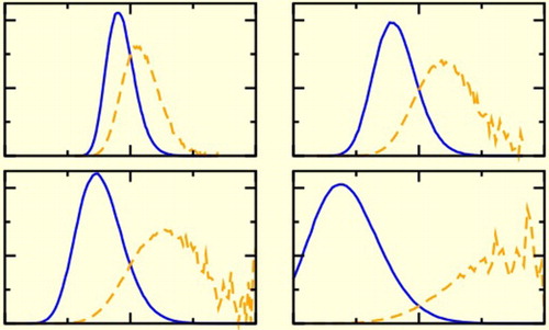
We now test our prediction that, as the length n of the trajectory used to compute the reweighting factor W increases, the distribution of W values sampled will broaden, making it hard to compute accurate results. Figure 3 (solid lines) shows histograms for computed from our simulations for n=20 (left panels) and n=50 (right panels). As predicted by our theoretical analysis, indeed approaches a normal distribution for large values of n and this distribution indeed broadens as n increases. Comparing results for different values of the target system death rate (top to bottom in Figure 3), we see that the distribution also broadens as decreases, i.e. as the target and reference system become more different from each other. This is because the distribution of values becomes wider as the reference system deviates further from the target system.

Figure 3. The functions (solid lines) and (dashed lines) for n=20 (a, c, e) and n=50 (b, d, f); and for (a, b), (c, d), and (e, f). Panels are also labelled directly by (, n), and these values of are also shown arrowed in Figure 4.

Figure 4. The ratio of the weighted estimate of the target mean copy number to the expected value, as varies, at fixed (this quantity should ). Each data point is a separate simulation along the lines of Figure 1. Two values of the trajectory length are explored, and the upward-pointing arrows indicate the values of used in Figure 3.

When computing weighted averages (as in Equation (1(1) )) what is important is actually , or since trajectories with high weight W contribute more to the average.² We therefore also plot in Figure 3 (dashed lines) the distribution of values of . Comparing the results for different trajectory lengths n=20 (left panels) and n=50 (right panels), we see that as the trajectory length increases, not only does broaden (solid lines) but also the peak in gets shifted further into the tails of . Thus for longer trajectories we become less likely to sample the relevant parts of , where the weight W is large. We also see the same effect upon decreasing (top to bottom panels in Figure 3); as the target and reference systems become more dissimilar, sampling trajectories with a high weight in the target system becomes less likely.³ Figure 3 rather dramatically underscores the importance of the extreme high weight trajectories in calculating weighted averages. Exactly the same kind of phenomenology is seen for Rosenbluth weights [36]. Indeed, Figure 3 closely mirrors Figure 2 in Ref. [38] for polymers localised in random media.

Figure 4 illustrates how the difficulty in sampling the relevant parts of leads to poor statistics when computing averages in the target system. Here, we plot trajectory reweighting simulation results for the ratio of the computed value of , to the analytical result (note that since this ratio is equal to ). As in Figure 3, results are shown for two values of the trajectory length, n=20 (dashed line) and n=50 (solid line), and for various values of . We first note that when is small (slow relaxation of the target system), there is a systematic deviation from the correct result ; this is because has not yet reached steady state. Increasing the trajectory length n from 20 to 50 indeed decreases this deviation. However, we pay a penalty for this in terms of the sampling error; the error bars on our data points become much larger for the longer trajectories. This reflects the increasingly poor sampling of the underlying W distribution (Figure 3). If we attempt to further reduce the systematic error for small values of by increasing n still further, for example to n=100, then we see so few of the important but exponentially rare high-weight trajectories that the results become statistically meaningless. This illustrates rather clearly the ‘Catch-22’ practical issue associated with trajectory reweighting for computing steady-state properties: for target systems with slow dynamics, long trajectories are needed, but because trajectory reweighting is an iterated importance sampling scheme, its statistical accuracy decreases, catastrophically, as the trajectory length increases.

4. Discussion

Trajectory reweighting provides an apparently elegant way to extend biased sampling methods developed for equilibrium steady states, to non-equilibrium systems whose dynamics do not obey detailed balance. By simulating a reference system, which is easier to sample than the target system of interest, one can obtain averages over the (un-simulated) target system by reweighting averages in the simulated reference system using reweighting factors computed from the reference system trajectories. The analysis presented here shows this is possible in principle, and that it does indeed work for the not-too-challenging test case of a birth–death process. For this particular problem though, it is clear that trajectory reweighting will never beat straightforward sampling: if the target system relaxes more slowly than the reference system ( in Figure 4) one comes up against the problem of poor sampling of the high-W trajectories (Figure 3); conversely if the target system relaxes faster than the reference system (), it is simply more efficient to simulate the target system directly. However, we expect trajectory reweighting has the potential to be useful for systems whose dynamics makes slow switches between alternative ‘basins of attraction’ (e.g. a genetic switch), since using a reference system that relaxes faster than the target system should allow better sampling of trajectories that switch between the basins.

Our work reveals the two significant practical issues which preclude the straightforward application of trajectory reweighting. First, the timescale to obtain unbiased estimates of reweighted quantities is still set by the target system. For example, to calculate steady-state averages in our toy model, one needs trajectory durations which are 2–3 times the relaxation time in the target system (; see Figures 2 and 4). We expect this rule-of-thumb to hold generally. Second, for long trajectories, the distribution of trajectory weights becomes extremely broad, and the weighted averages that we need to compute are sensitive to the rarely visited high-weight region. In our toy model this is exemplified in Figure 3. This problem becomes acute for target systems which involve barrier-crossing events, such as genetic switches. Since the barrier-crossing frequency is very small, the relaxation times are very long. Then, we cannot escape from the fact that very lengthy trajectories are required to compute steady-state averages in such target systems, even if the reference system equilibrates rapidly.

It is important to note that this problem is specific to the use of trajectory reweighting for steady-state system properties. Trajectory reweighting has been successfully applied in numerous other contexts, including financial mathematics [16], rare event analysis in applied mathematics [16,17], and first-passage time problems [30–33]. The essential difference is that these problems are characterised by short-duration trajectories. For sampling of short trajectories, the measurement statistics of infrequent events can be drastically improved by generating a large number of successful but biased trajectories, even though these may carry a low weight once the bias is removed. This variance-reduction mechanism was cogently argued by Gillespie et al. [30]. In contrast, to sample steady-state properties, long-duration trajectories have to be reweighted, with the associated sampling problems discussed here.

We have noted that there is a close analogy between computing trajectory weights, and Rosenbluth sampling for chain macromolecules. This suggests a possible way forward. In the Rosenbluth method, inefficient sampling of high-weight polymer configurations was resolved by the development of the pruned-enriched Rosenbluth method (PERM) [1,37], and its descendant flat-histogram PERM [15,44]. To apply this in the present situation, one would follow an ensemble of trajectories, and in order to keep the weights in the desired region in (Figure 3), at intermediate times discard trajectories with low weights, and clone trajectories with high weights. The added complications are the increased bookkeeping required to keep track of a variable number of trajectories, and the need to fine-tune the hyper-parameters in the algorithm. We note that PERM applied to this problem does not necessarily avoid the issue that the sampling time is set by the target system, thus for instance for a genetic switch we expect one would need to sample for 2–3 times the waiting time to cross the barrier. However, by diminishing or removing the barriers in a rugged probability landscape, we expect that the use of trajectory reweighting will distribute the sampling effort more effectively over state space, leading to more accurate calculation of steady-state probability distributions. Undoubtedly this will only become clear with further and more detailed investigations, which we leave for future work. Another possible avenue to explore is the use of simultaneous trajectory reweighting across multiple systems, as in the extended bridge sampling method [45].

Acknowledgments

We thank H. Touchette for discussions and a critical reading of an earlier version of this manuscript, D. Frenkel for drawing attention to the analogy to Rosenbluth weights, and T. Prellberg for highlighting to us the advanced PERM-based methods for polymer sampling.

Disclosure statement

PBW discloses a substantive (>$10k) stock holding in Unilever PLC.

Additional information

Funding

R.J.A. was supported by a Royal Society University Research Fellowship and by Engineering and Physical Sciences Research Council (EPSRC) under grants EP/I030298/1 and EP/J007404/1. P.B.W. thanks the Higgs Centre for Theoretical Physics for funding travel under the Associate Member program. 

Notes

1 Note that is only 3% different from , whereas and differ by 40%, so replacing by in Equation (10(10) ) would make an indiscernible difference to the goodness of the fit.

2 Since we are dealing with probability distributions, . Multiplying through by W shows that is the correct quantity to think about in this context.

3 Note that poor sampling of is distinct from the problem that arises when there is poor overlap between the reference and biased probability distributions.

Appendices

A.1. Appendix 1. Formalism for trajectory reweighting

Here, we derive Equation (5(5) ) and show formally that the relaxation time of the reweighting factor W is controlled by the dynamics of the target system rather than the reference system. We define and as the probabilities that, respectively, the target and reference system are in microstate after n steps. We can leave the starting state unspecified. The steady-state probability distributions and in the main text are the large n limits of and . In addition to these, we define (A1) This is the mean weight per trajectory of length n that ends in . In the limit , it is the quantity that features on the right-hand side of Equation (5(5) ) in the main text.

The actual weight in microstate is obtained by multiplying by the probability that a trajectory ends in microstate , namely . An evolution equation for this can be written down by analogy to §1 of the Supplemental Material for Ref. [24], or Equation (8) in Ref. [25]. It is (A2) This looks formidable but can be taken apart piece by piece. The first factor in the sum on the right-hand side is the total weight in microstate after n−1 steps. The second factor is the probability that this weight subsequently propagates to . The third factor arises because the weight is updated at each step by multiplying by the relative transition probabilities . Cancelling factors of , Equation (A2(A2) ) simplifies to (A3) This can be compared to the evolution equation for , which is (A4) This simply expresses the fact that plays the role of a transition probability matrix. On inspection, Equations (A3(A3) ) and (A4(A4) ) are structurally identical, and (unless we have chosen a pathological case) converge to identical steady-state solutions to within a multiplicative constant, irrespective of the choice of initial conditions. This then implies (A5) or, recalling the definition in Equation (A1(A1) ), (A6) This proves the intended result, Equation (5(5) ) in the main text.

As a corollary to all this, we note that the convergence to steady state in Equations (A3(A3) ) and (A4(A4) ) is governed by the spectral properties of , that is to say by the target system, not the reference system. The implications of this are discussed in the main text.

Appendix 2. Reweighting algorithm for birth–death process

We simulate the birth–death process in Equation (8(8) ) using the Gilespie kinetic Monte-Carlo algorithm [43]. At some point in time, suppose there are x copies of . The transition rates (the reaction ‘propensities’) are (A7) Accordingly, we select a time step from an exponential distribution , where , and reaction channel with probabilities . We advance time by and update x according to the chosen reaction channel. This completes one update step.

The transition probability for this update step is (A8) We omit the ‘measure’ , which in any case cancels out below.

Now suppose we are simulating the reference system with death rate , and we wish to reweight to a target system with a different death rate . The ratio of transition probabilities is then, specifically, (A9) Since λ is the same in the target and reference systems, the λ-dependence cancels in this.

Thus in order to reweight the system, we simulate the system using the standard Gillespie algorithm, but after making the choice of time step and reaction channel, we compute the ratio according to Equation (A9(A9) ). We maintain a circular history array of length n, and keep a pointer into this history array. When the value of is calculated, it is stored in the array at the location corresponding to the current value of the pointer, which is then incremented (and reset to the beginning if it goes past the end of the array). The effect of this is that the oldest value of is replaced by the most recent value, whilst keeping all the intermediate values.

For steady-state problems we typically (re)set time to t=0 and iterate the above algorithm until , where is some sampling interval. At that point we make a note of the state of the system (i.e. the value of x in this case) and the reweighting factor W, which is simply the product of the values stored in the history array at that point in time. We keep track of these values of x and W and use them to compute the desired averages, and .

The value of should be chosen so that the system is fully relaxed between samples. This ensures statistical independence of the sampling points. Additionally, we should make sure is sufficiently large so that the history array is completely refreshed between samples (this also has the side-effect of ‘pump-priming’ the array from a cold start). In the present study we set equal to the larger of or .

Appendix 3. Extreme value statistics and trajectory weights

Suppose that we simulate N trajectories of length n. This generates N samples of the reweighting factor W, where is normally distributed with some mean m and variance v. Although we can get good coverage of the underlying normal distribution with a moderate value of N, the problem arises because we need to sample the tail of the normal distribution when constructing averages weighted with .

The W-weighted averages we are trying to calculate are governed by an overall multiplier of the form (A10) This comprises the weight multiplied by the distribution of values (i.e. the same as in Figure 3). Equation (A10(A10) ) has a maximum at z=m+v. To achieve good statistics, we need to sample the tail of the z-distribution in this vicinity. This is a very stringent requirement, and in particular is not simply satisfied by reaching out to some multiple of the standard deviation beyond the mean.

This consideration can be expressed in another way by considering the extreme value statistics of z [46,47]. Recall that for N samples of a normal distribution, the typical maximum value reached (the ‘high water mark’) is . If we demand that , then at least the ‘high water mark’ of the sampled z values is beyond the peak in Equation (A10(A10) ). This translates into , or . Therefore for , with some coefficient β. Turning this around it means that the relevant trajectories which contribute to the weighted averages become exponentially rare as n increases, supporting the claim made in the main text.

References

- D. Frenkel and B. Smit, Understanding Molecular Simulation: From Algorithms to Applications, 2nd ed. (Academic, San Diego, CA, 2002).
- G.M. Torrie and J.P. Valleau, J. Comp. Phys. 23, 187 (1977).
- M.R. Evans, D.P. Foster, C. Godrèche and D. Mukamel, Phys. Rev. Lett. 74, 208 (1995).
- K. Stratford, R. Adhikari, I. Pagonabarraga, J.C. Desplat and M.E. Cates, Science 309, 2198 (2005).
- A. Arkin, J. Ross and H.H. McAdams, Genetics 149, 1633 (1998).
- M. Santillán and M.C. Mackey, Biophys. J. 86, 75 (2004).
- M.J. Morelli, P.R. ten Wolde and R.J. Allen, Proc. Natl. Acad. Sci. USA 106, 8101 (2009).
- P.B. Warren and P.R. ten Wolde, J. Phys. Chem. B 109, 6812 (2005).
- A. Warmflash, P. Bhimalapuram and A.R. Dinner, J. Chem. Phys. 127, 154112 (2007).
- C. Valeriani, R.J. Allen, M.J. Morelli, D. Frenkel and P.R. ten Wolde, J. Chem. Phys. 127, 114109 (2007).
- A. Dickson, A. Warmflash and A.R. Dinner, J. Chem. Phys. 130, 074104 (2009).
- A. Dickson, A. Warmflash and A.R. Dinner, J. Chem. Phys. 131, 154104 (2009).
- A. Dickson and A.R. Dinner, Annu. Rev. Phys. Chem. 61, 441 (2010).
- R.J. Allen, C. Valeriani and P.R. ten Wolde, J. Phys. Condens. Matter. 21, 463102 (2009).
- N.B. Becker, R.J. Allen and P.R. ten Wolde, J. Chem. Phys. 136, 174118 (2012).
- S. Asmussen and P.W. Glynn, Stochastic Simulation: Algorithms and Analysis (Springer, New York, 2007).
- H. Touchette, A Basic Introduction to Large Deviations: Theory, Applications, Simulations; 2012. Arxiv: 1103.4146v3.
- P. Glasserman, Gradient Estimation via Perturbation Analysis (Springer, New York, 1990).
- T. Wang and M. Rathinam, SIAM/ASA J. Uncertainty Quant. 4, 1288 (2016).
- C. Jarzynski, Phys. Rev. Lett. 78, 2690 (1997).
- G.E. Crooks, Phys. Rev. E 60, 2721 (1999).
- S.X. Sun, J. Chem. Phys. 118, 5769 (2003).
- P.B. Warren and R.J. Allen, J. Chem. Phys. 136, 104106 (2012).
- P.B. Warren and R.J. Allen, Phys. Rev. Lett. 109, 250601 (2012).
- P.B. Warren and R.J. Allen, Entropy 16, 221 (2014).
- L. Onsager and S. Machlup, Phys. Rev. 91, 1505 (1953).
- A.B. Adib, J. Phys. Chem. B 112, 5910 (2008).
- B. Harland and S.X. Sun, J. Chem. Phys. 127, 104103 (2007).
- H. Kuwahara and I. Mura, J. Chem. Phys. 129, 165101 (2008).
- D.T. Gillespie, M. Roh and L.R. Petzold, J. Chem. Phys. 130, 174103 (2009).
- M.K. Roh, D.T. Gillespie and L.R. Petzold, J. Chem. Phys. 133, 174106 (2010).
- B.J. Daigle Jr, M.K. Roh, D.T. Gillespie and L.R. Petzold, J. Chem. Phys. 134, 044110 (2011).
- M.K. Roh, B.J. Daigle Jr, D.T. Gillespie and L.R. Petzold, J. Chem. Phys. 135, 234108 (2011).
- S. Plyasunov and A. Arkin, J. Comput. Phys. 221, 724 (2007).
- M.N. Rosenbluth and A.W. Rosenbluth, J. Chem. Phys. 23, 356 (1955).
- J. Batoulis and K. Kremer, J. Phys. A: Math. Gen. 21, 127 (1988).
- P. Grassberger, Phys. Rev. E 56, 3682 (1997).
- P. Grassberger, J. Chem. Phys. 111, 440 (1999).
- W. Feller, An introduction to Probability Theory and Its Applications, Vol. 1, 3rd ed. (Wiley, New York, 1968).
- J. Aitchison and J.A.C. Brown, The Lognormal Distribution (CUP, Cambridge, 1957).
- M.J. Morelli, S. Tanase-Nicola, R.J. Allen and P.R. ten Wolde, Biophys. J. 94, 3413 (2008).
- H. Touchette (private communication).
- D.T. Gillespie, J. Phys. Chem. 81, 2340 (1977).
- T. Prellberg and J. Krawczyk, Phys. Rev. Lett. 92, 120602 (2004).
- D.D.L Minh and J.D. Chodera, J. Chem. Phys. 131, 134110 (2009).
- E.J. Gumbel, Statistics of Extremes (Columbia University Press, New York, 1958).
- S. Coles, An Introduction to Statistical Modeling of Extreme Values (Springer, London, 2001).