Neural-network-based order parameters for classification of binary hard-sphere crystal structures

ABSTRACT

Identifying crystalline structures is a common challenge in many types of research. Here, we focus on binary mixtures of hard spheres of various size ratios, which stabilise a range of crystal structures with varying complexity. We train feed-forward neural networks to distinguish different crystalline and fluid environments on a single-particle basis, by analysing vectors composed of several averaged local bond order parameters. For all size ratios considered, we achieve a classification accuracy above for all phases, meaning that our method is completely general and able to capture structural differences of a wide range of binary crystals.

GRAPHICAL ABSTRACT

KEYWORDS:

• Binary hard spheres
• neural networks
• order parameters
• colloids

1. Introduction

The study of many structural and dynamic phenomena involving crystalline phases, including nucleation and growth, melting and grain boundary dynamics, relies on our ability to determine whether or not a particle is part of a crystalline cluster or domain. In bulk, crystalline solids can be straightforwardly distinguished from fluids as they exhibit both translational and bond-orientational order. Moreover, the difference between various crystal structures is readily accessible by determining their unit cell. However, on a single-particle level, the distinction between a fluid and a crystal is much less clear: in a small crystalline cluster, as might exist during nucleation or in a polycrystalline material, long-range translational or bond-orientational order is not present.

One of the more common methods for identifying crystalline particles is based on local bond order and finds its origins in a 1982 paper by Steinhardt, Nelson, and Ronchetti [1]. They introduced bond-orientational order parameters suitable for studying bond-orientational order in liquids and glasses. As a starting point, they defined for each particle a set of bonds to its nearby neighbours. They then expanded the distribution of bonds in the system in terms of the spherical harmonics of order l, and used this expansion to construct quadratic and cubic rotationally invariant quantities that measure specific bond-order symmetries in the system, generally referred to as and , respectively. This idea was inspired by the Landau expansion of the free-energy difference between a bond-oriented (crystalline) and a fluid phase in terms of the same spherical harmonic functions (see e.g. [2]). Subsequently, this concept was extended to analyse structure on a single-particle level by Ten Wolde, Ruiz-Montero, and Frenkel [3,4]. The resulting local bond-order parameters allow for both the identification of particles in environments corresponding to a specific crystal structure, and to identify clusters of particles belonging to the same crystalline domain. In a later extension by Lechner and Dellago [5], it was shown that the reliability of these order parameters in the presence of thermal fluctuations could be significantly improved by averaging the bond order parameter of each particle with that of its nearby neighbours. Bond order parameters have played a significant role in our understanding of single-component phase behaviour, and have been a particularly valuable tool in the study of hard spheres, arguably the simplest model system forcrystallisation. In this context, bond order parameters have been instrumental in developing new insights into, e.g. the nucleation rate [6], the shape of pre-critical nuclei [7], nucleation from a glass [8] and the role of confinement [9]. However, in most of these studies, the focus lies primarily on single-component systems, where all relevant crystal structures are easy to predict and have relatively simple unit cells. In contrast, bond order parameters for binary phases, which can be significantly more complex, have received much less attention.

The equilibrium phase behaviour of binary hard-sphere mixtures has been well characterised in the literature. One of the first observations of binary colloidal crystals was made by Murray and Sanders in naturally occurring Brazilian gem opals [10,11]. They observed the formation of a range of binary crystals, including NaCl, AlB and NaZn (ico-AB), all of which were later confirmed to be stable in binary hard-sphere mixtures [12–16]. Since then, our understanding of the phase behaviour of binary hard spheres has come a long way, and we now have theoretical phase diagrams for a wide range of size ratios, largely backed up by experimental observations [15,17,18]. These studies have found regions of stability for binary liquids, monodisperse face-centred-cubic (fcc) crystals, binary crystal phases NaCl, NaZn, AlB, the Laves phases (MgCu, MgZn, MgNi), an AB phase with no atomic analogue, as well as substitutional and interstitial solid solutions. However, in comparison to single-component hard spheres, our knowledge of the crystallisation dynamics of binary crystals is still severely limited. One of the puzzle pieces currently missing in the literature are well-performing order parameters that identify, on a single particle level, the complex local environments associated with binary hard-sphere crystal phases.

In this paper, we use machine learning to develop order parameters, based on the bond order parameters, to distinguish crystalline environments in binary mixtures of hard spheres. Recently, machine learning has been shown to be an extremely promising approach in the study of phase behaviour, both for predicting phase transitions as well as for developing new order parameters [19–26]. Research on the uses of machine learning for designing order parameters can be loosely broken into two categories: supervised and unsupervised machine learning. In the context of supervised machine learning, it has recently been demonstrated that neural networks could be used as order parameters for recognising various crystalline order in single-component systems, including Lennard Jones, Yukawa and water potentials [23,24]. These examples are very similar to the situation examined in this paper: assuming that we know a priori which crystalline phase we want to be able to distinguish, neural networks are trained to recognise that local order. These examples used different types of ‘local’ environment characterisations, including bond order parameters [24] and symmetry functions [23]. The unsupervised learning algorithms function quite differently and are designed to identify the distinctive groups of local environments that are present in the system – without a priori knowledge of the possibilities. This has been applied to, e.g. single component systems [25], and 2d binary systems [26].

Here, we train single-layer neural networks to recognise different particle environments, corresponding to fluid or crystalline phases, in simulations of binary hard-sphere mixtures. In particular, we perform Monte Carlo simulations of binary hard-sphere mixtures at three different size ratios and 0.82, with the diameter of the small (large) species. These size ratios were chosen because they cover a number of distinct stable binary crystal structures. For each phase, we considered different packing fractions, η, defined as (1) where is the stoichiometry and is the number density. We then characterise the environments of particles in different phases using the averaged bond order parameters introduced by Lechner and Dellago [5], and train neural networks to identify distinct local environments that occur in the different crystal structures. Finally, we test these networks on separate simulations and quantify their accuracy.

The remainder of this paper is organised as follows. In Section 2, we describe the bond order parameters in detail. In Section 3, we outline the setup of the neural networks used in this paper. In Section 4, for each size ratio, we examine the investigated crystal structures and their local environments, and describe the associated neural network. Finally, in Section 5, we discuss the performance of the trained neural networks. A summary and discussion follows in Section 6.

2. Bond order parameters

To characterise the local environment of each particle, we use the averaged bond order parameters introduced by Lechner and Dellago [5]. First, we define for any given particle i the complex quantities (2) where are the spherical harmonics of order l, with m an integer that runs from m=−l to m=+l. Additionally, is the vector from particle i to particle j, and is the set of nearest neighbours of particle i, which contains particles. Then, the averaged are defined as (3) where the sum runs over all nearest neighbours of particle i as well as particle i itself. Averaging over the nearest neighbour values of results effectively in also taking next-nearest neighbours into account. Finally, we define rotationally invariant quadratic and cubic order parameters as (4) (5) where the term in parentheses in Equation (5(5) ) is the Wigner symbol. The quantities in Equations (4(4) ) and (5(5) ) are real, translationally and rotationally invariant, and, depending on the choice of l, are sensitive to different crystal symmetries. Our description of the local environment of particle i consists of a vector of 24 such bond order parameters arranged in the following order: (6) for large (small) particles, with and consisting of only even values of l. Here and represent the averaged bond order parameters calculated considering all the nearest neighbours of the particles, while and are calculated considering only the large (small) nearest neighbours of large (small) particles.

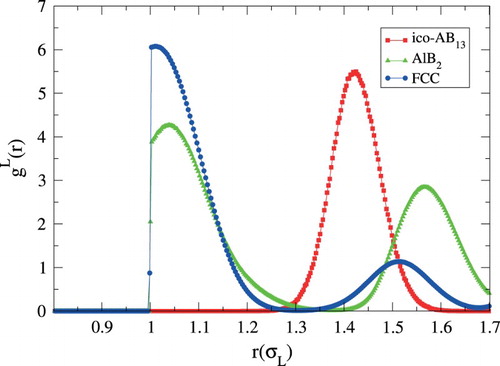
Thus far, we have not discussed the definition of a nearest neighbour, as used in the definition of the bond order parameters. There are a number of different avenues for identifying nearest neighbours. The simplest method, and one we use in this paper, relies on using a fixed cutoff radius , such that all particle closer than this distance are considered nearest neighbours. Ideally, this cutoff radius is chosen as the distance at which the radial distribution function has its first minimum. When considering different crystal structures, however, the minima often occur at different distances, so that no choice of works perfectly for all crystals (see Figure 1). In this paper, we choose by trying to maximise the number of included first neighbours and to minimise the number of included second neighbours for all crystals. This method has the advantage that it is computationally very cheap and it is symmetric, i.e. i is a neighbour of j if and only if j is a neighbour of i. However, is system and density dependent, so that it has to be tuned for every particular case requiring prior knowledge of the system(s) under study. Additionally, the cutoff is defined for the entire system and, as such, is not an optimal choice for systems with large density gradients or interfaces, such as can occur in nucleation studies.

Figure 1. Radial distribution functions of large particles of ico-AB (), AlB () and FCC () hard spheres crystals.

Another standard method for determining nearest neighbours is the Voronoi construction [27], which has the advantage that it is parameter free. However, it is also relatively computationally expensive, and in this paper we have instead opted to make use of a recently introduced alternative parameter-free nearest-neighbour criterion, called SANN (solid angle nearest neighbour) [28]. In this approach, an effective individual cutoff is found for every particle in the system based on its local environment. The algorithm can briefly be described as follows.

First, the particles surrounding i are ordered such that . Then, starting with the particle closest to i, a solid angle is associated to every potential neighbour j. Finally, SANN defines the neighbourhood of particle i as consisting of the nearest (i.e. closest) m particles such that the sum of their solid angles equals at least . For a complete description of the algorithm, see Ref. [28].

This method is not inherently symmetric, i.e. j might be a neighbour of i while i is not a neighbour of j. However, symmetry can be enforced by either adding j to the neighbours of i or removing i from the neighbours of j. In this study, we applied the latter solution. The computational cost of SANN only slightly exceeds that of a cutoff distance, making it suitable for on-the-fly use in simulations. Moreover, since it is a parameter free method, it is suitable for systems with inhomogeneous densities. The only inconvenience we encountered with SANN is that, in some cases, some second shell neighbours are also included in the nearest-neighbour lists.

3. Neural networks for the classification of binary hard spheres crystals

Our goal is to develop algorithms which are able to distinguish different crystalline environments for binary hard-sphere systems on a single-particle basis. To this end, we employ feed-forward neural networks, which are general purpose algorithms that ‘learn’ the properties of a specific classification problem from labelled data. In particular, we consider single-layer neural networks (SLNN) with a Softmax activation function and cross-entropy error function. For a detailed description of how such a network is implemented, see the Supplemental Information. SLNNs are one of the simplest forms of feed-forward neural networks and are able to efficiently find linear separations of data in high dimensional spaces, provided that the data are indeed linearly separable. Using such a simple structure instead of more complex ones has some important advantages. The training is easy – in the sense that it does not require advanced techniques for function minimisation – and computationally cheap, and the risk of overfitting¹ is low. The only limitation is that they fail on problems which are inherently nonlinear, but as we will show, this is not a problem in this work.

We examine binary hard-sphere mixtures of three different size ratios ( and 0.82). For each size ratio, we train an SLNN to distinguish the different local environments that occur in the stable phases. The network takes as its input the vector in Equation  (6(6) ), namely our description of the local environment of one particle. As its output, it produces a number for each potential local environment, indicative of the likelihood the particle is in this environment. The determined particle environment is then considered to be the one with the highest likelihood.

To train the network, its internal parameters are optimised based on information contained in a so-called ‘training set’. The training set is constructed by determining a representative sample of of particles in configurations in each known phase. In particular, we perform Monte Carlo simulations in the canonical ensemble (constant number of particles N, composition x, volume V and temperature T), for each of the stable phases under consideration. From each simulation, we save 100 independent snapshots, and calculate for each particle. Note that since diffusion in the crystal phases is essentially absent, we know the correct environment for each particle. This knowledge, combined with the set of , forms our training set. The number of distinct local environments depends on the specific size ratio, as we will discuss in the following section.

We calculate bond order parameters both using a fixed cutoff distance and the SANN algorithm, resulting in two training sets and hence two distinct SLNNs. When examining their performance, we will refer to these networks as the ‘cutoff networks’ and ‘SANN networks’, respectively. The chosen cutoff distances for the cutoff networks are listed in Table 1, where is the cutoff used to identify all the nearest neighbours of the particles, to identify only the large nearest neighbours of large particles, and to identify the small nearest neighbours of small particles. These cutoff distances are chosen as described in Section 2 by looking at the first minimum of the radial distribution functions of both species (large and small particles), of only large particles, and only small particles, respectively.

Table 1. Cutoff distances used for different size ratios.

α
0.45	1.3	1.3	1.3
0.54	1.3	1.45	0.83
0.82	1.3	1.3	1.1

4. Crystal structures

In this section, for each size ratio we describe the stable crystal structures, their associated local environments, and the details of the SLNNs we trained.

4.1. Size ratio

We first consider binary hard spheres with size ratio . As shown in Ref. [29], stable phases with this size ratio are NaCl and AlB binary crystals, FCC crystals of large or small particles, and the binary fluid. Unit cells for these phases are shown in Figure 2. For the crystal phases, we distinguish four local environments: one for the FCC phase (which is identical for the large and small particles), one for NaCl (where both species are on identical FCC sublattices), and two for AlB corresponding to the large and small particle environments.

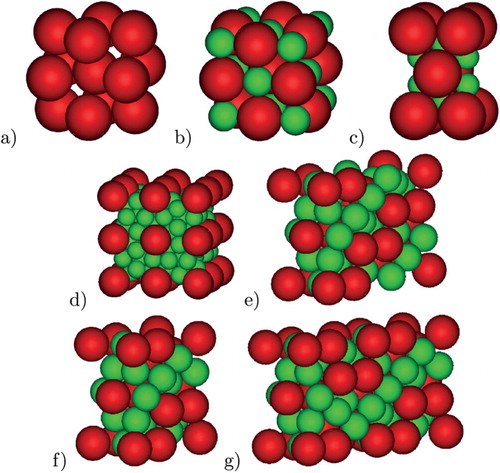
Figure 2. Unit cells for (a) FCC, (b) NaCl, (c) AlB, (d) ico-AB, (e) MgCu, (f) MgZn, (g) MgNi.

Hence, we set up an SLNN with 24 inputs and 5 outputs. The 24 inputs correspond to the length of the vector , while the output corresponds to the following 5 environments:

• Label 0: particles of NaCl;

• Label 1: large particles of AlB;

• Label 2: small particles of AlB;

• Label 3: particles of the binary fluid;

• Label 4: particles of FCC.

We train the network using sets of from MC simulations of all four phases. For the NaCl, AlB and FCC crystals, the simulations were performed at packing fractions , and , respectively, while for the binary fluid we used a packing fraction of and a stoichiometric ratio .

4.2. Size ratio

We now consider binary hard spheres with size ratio . As shown in Ref. [30], stable phases with this size ratio are ico-AB and AlB binary crystals, FCC crystals of large or small particles, and the binary fluid (see Figure 2). As discussed in the previous section, there are a total of three local environments in FCC and AlB. In ico-AB, there is a single environment for the large particles, but multiple environments for the small particles. However, it turns out that grouping all small ico-AB particles under one label results in excellent identification of the particle environments.

Hence, for this size ratio the SLNN has six outputs, corresponding to the following environments:

• Label 0: large particles of ico-AB;

• Label 1: small particles of ico-AB;

• Label 2: large particles of AlB;

• Label 3: small particles of AlB;

• Label 4: particles of FCC;

• Label 5: particles of the binary fluid.

To obtain the training data, the MC simulations for ico-AB, AlB and FCC crystals were performed at packing fractions of , and , respectively, while for the binary fluid we used a packing fraction of and a stoichiometric ratio .

4.3. Size ratio 0.82

Finally, we consider binary hard spheres with size ratio . As shown in Refs. [31,32], stable phases for this size ratio are the MgZn Laves phase, the binary fluid, and the FCC crystals of only large or small particles. Interestingly, as shown in Ref. [32], there are two other Laves phases competing with MgZn for stability: MgCu and MgNi. These structures are very similar to MgZn, but correspond to different stackings of the same crystalline planes. In particular, the arrangement of planes in MgNi is a combination of the arrangements in MgCu and MgZn. The free-energy difference between these phases is only on the order of per particle, and hence it is likely that mixtures of these phases would show up in, e.g. nucleation studies. Hence, in addition to the fully stable phases, we include MgCu and MgNi in our analysis. Unit cells of the investigated phases are shown in Figure 2.

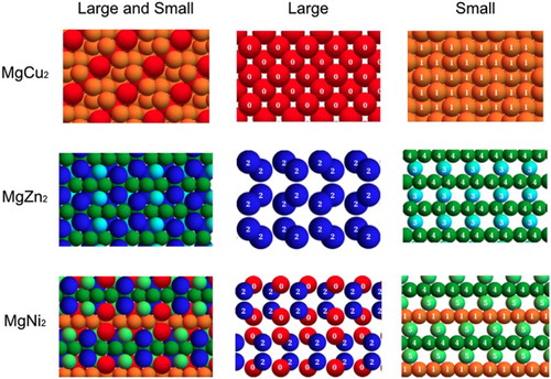
A closer analysis of the local environments in the Laves phases reveals a complication in the unique identification of the MgNi environments when only first shell neighbours are taken into account. In particular, by computing the vectors for the perfect crystal configurations of the three Laves phases, we found that most of the environments in MgNi are also present in either MgZn or MgCu – where by ‘same environment’ we mean that the vectors are essentially equal. This is shown in Figure 3, where particles of the Laves phases are coloured according to their environment, as described by . There are two possible solutions to this. First, one can systematically take into account an additional shell of neighbours when calculating . When second-nearest neighbours are systematically taken into account, bond order parameters are able to capture the different stackings and the local environments in the different Laves phases are distinguishable. Training a neural network with such a set indeed results in an excellent identification of all three Laves phases. The second approach is to simply identify which local environment (as represented in Figure 3) each particle is in, regardless of crystal structure. The environments of neighbouring particles can subsequently be used to determine the underlying lattice. As we would like to base particle identification purely on the immediate environment of the particle, we here focus on the second solution.

Figure 3. Perfect crystal configurations of the three Laves phases. Colours represent the distinct local environments we identify from bond order parameters calculations, considering only first shell neighbours.

Hence, for this size ratio, our SLNN has eight outputs, corresponding to the following local environments, as labeled in Figure 3:

• Label 0: large particles of MgCu and half of the large particles of MgNi (particles in Figure 3);

• Label 1: small particles of MgCu and some of the small particles of MgNi (particles in Figure 3);

• Label 2: large particles of MgZn and half of the large particles of MgNi (particles in Figure 3);

• Label 3: some small particles of MgZn (particles in Figure 3);

• Label 4: some small particles of MgZn and small particles of MgNi (particles in Figure 3);

• Label 5: some small particles of MgNi (particles in Figure 3);

• Label 6: particles of the binary fluid;

• Label 7: particles of FCC.

As shown in Figure 3, the individual Laves phases can then be easily distinguished by looking at the labels of the large particles. For MgCu, all large particles have label 0 (red), for MgZn, they have label 1 (blue), and in MgNi the two labels are evenly mixed.

MC simulations to train the network were performed using a packing fraction of for the Laves phases, for the FCC crystal, and and stoichiometry for the binary fluid.

5. Results

To train our SLNNs and assess their performance, we make use of a cross-validation procedure. The averaged overall accuracies of the cutoff and SANN networks at each size ratio, as well as the accuracies related to each specific label, are shown in Table 2. In all cases we reach an overall accuracy above , meaning that our method is completely general and able to capture structural differences of a wide range of binary crystals. Looking closer at the specific phases, we find that in general, the fixed cutoff preforms slightly better than SANN, and postulate that this arises due to the tendency of SANN to occasionally include one or more neighbours from the second neighbour shell. As these additional particles are located at positions different from those normally associated with the first-shell neighbours, this impacts the bond order parameters for the central particle in an unpredictable fashion, leading to a misclassification.² Nonetheless, we find that all individual phases are recognised correctly more than 98% of the time, even with SANN, which we consider to be excellent performance.

Table 2. Average accuracies of the networks computed with the cross-validation procedure.

	Labels
Network	Overall	0	1	2	3	4
Cutoff
SANN
	Labels
Network	Overall	0	1	2	3	4	5
Cutoff
SANN
	Labels
Network	Overall	0	1	2	3	4	5	6	7
Cutoff
SANN

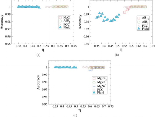
The tests of our SLNNs reported in Table 2 are all performed at exactly the same packing fraction as the one that was used for training the networks. As a result, it is not a priori clear whether the trained networks are an appropriate order parameter for crystals at different packing fractions. In order to test this, for each size ratio, we examine the performance of the network over a wide range in packing fractions and report the results in Figure 4. Note that here we limit our attention to the order parameter using SANN, in order to avoid having to recalculate the cutoff range for each packing fraction. In all cases, the accuracy of the network is found to be higher than 98%, confirming that SLNNs are robust to changes in density.

Figure 4. Performance of the order parameters as a function of density, for binary hard sphere mixtures with size ratio 0.45 (a), 0.54 (b) and 0.82 (c), using the SANN networks.

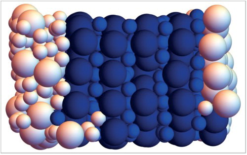
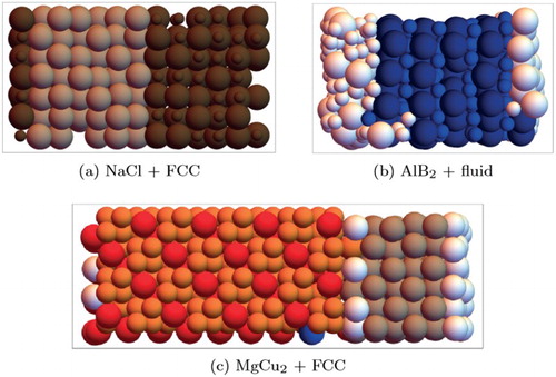
To further test the SANN networks, and in particular their performance in systems with interfaces, we applied them to snapshots from additional MC simulations of systems with a coexistence of two phases. In particular, we examined coexistences of the following: (i) NaCl and FCC for size ratio (Figure 5a), (ii) AlB and fluid for size ratio (Figure 5b), and finally MgCu and FCC for size ratio (Figure 5c). Note that the networks have not been trained to recognise particles at the interface and, furthermore, we do not have a reference output in order to compute the accuracy of the networks for such simulations. Nonetheless, in all cases the bulk phases are correctly classified, while, as expected, some disordered particles at the interface are classified as being fluid (white).

Figure 5. Particle classification for configurations of binary hard sphere mixtures with size ratio 0.45 (a), 0.54 (b) and 0.82 (c), using the SANN networks. In each configuration, two phases coexist as indicated. Particles identified as being in the fluid phase are white.

The final trained networks using the SANN nearest-neighbour criterion are included as a Python code in the Supporting Information (SI). The detailed parameters of the trained network are included in the SI as well.

6. Conclusion

In this study, we trained feed-forward neural networks to function as order parameters that ‘learn’ to distinguish different crystalline and fluid environments for binary mixtures of hard spheres on a single-particle basis, by analysing vectors composed of 24 averaged local bond order parameters. We found that for each size ratio, a simple, single-layer neural network was sufficient to distinguish all phases we explored.

We compared the behaviour of the neural networks with two different methods for determining nearest neighbours, namely a fixed cutoff, and the SANN. We found that both methods performed well, with the fixed cutoff slightly outperforming SANN. Nonetheless, the ‘parameter-free’ nature of SANN makes it much more flexible and suitable for use in systems containing variations in density. Our results demonstrate that the networks using SANN perform well over the entire range of stability of the explored phases and are capable of locating the interface between two coexisting phases. This makes them ideal for the analysis of both experimental and simulation data in fields ranging from crystal growth to interfacial phenomena. Moreover, once trained, the order parameter calculations are rapid, making such a network suitable, not only for post processing of data but also for on the fly calculations in, e.g. computational nucleation studies. The largest computational cost is by far in evaluating the bond order parameters.

Our results demonstrate the wide applicability of feed-forward neural networks for recognising the complex particle environments associated with multicomponent crystals, for which effective order parameters are not always known. The training of the networks used here takes mere seconds on a modern desktop computer and hence can easily be repeated for systems with different interactions and/or size ratios.

Acknowledgments

We dedicate this paper to Daan Frenkel in honour of his 70th birthday. We thank Michiel Hermes and Marjolein Dijkstra for useful discussions.

Disclosure statement

No potential conflict of interest was reported by the authors.

Additional information

Funding

L. F. and E. B. gratefully acknowledge funding from the Netherlands Organisation for Scientific Research (NWO) [grant number 16DDS004].

Notes

1 Overfitting refers to modelling a particular set of data too well. In machine learning, overfitting happens when a model learns the details and noise in the training data to the extent that it negatively impacts the performance of the model on new data.

2 This should be contrasted with intentionally and systematically training the network on data that takes into account the second-shell neighbours.

References

- P.J. Steinhardt, D.R. Nelson and M. Ronchetti, Phys. Rev. B 28, 784 (1983). doi: 10.1103/PhysRevB.28.784
- S. Goshen, D. Mukamel and S. Shtrikman, Solid State Commun. 9, 649 (1971). doi: 10.1016/0038-1098(71)90237-7
- P.R. Ten Wolde, M.J. Ruiz-Montero and D. Frenkel, Phys. Rev. Lett. 75, 2714 (1995). doi: 10.1103/PhysRevLett.75.2714
- P.R. Ten Wolde, M.J. Ruiz-Montero and D. Frenkel, J.Chem. Phys. 104, 9932 (1996). doi: 10.1063/1.471721
- W. Lechner and C. Dellago, J. Chem. Phys. 129, 114707 (2008). doi: 10.1063/1.2977970
- S. Auer and D. Frenkel, Nature 409, 1020 (2001). doi: 10.1038/35059035
- U. Gasser, E.R. Weeks, A. Schofield, P.N. Pusey and D.A. Weitz, Science 292, 258 (2001). doi: 10.1126/science.1058457
- E. Zaccarelli, C. Valeriani, E. Sanz, W.C.K. Poon, M.E. Cates and P.N. Pusey, Phys. Rev. Lett. 103, 135704 (2009). doi: 10.1103/PhysRevLett.103.135704
- B. De Nijs, S. Dussi, F. Smallenburg, J.D. Meeldijk, D.J. Groenendijk, L. Filion, A. Imhof, A. Van Blaaderen and M. Dijkstra, Nat. Mater. 14, 56 (2015). doi: 10.1038/nmat4072
- J. Sanders and M. Murray, Nature 275, 201 (1978). doi: 10.1038/275201a0
- M. Murray and J. Sanders, Philos. Mag. A 42, 721 (1980). doi: 10.1080/01418618008239380
- M.D. Eldridge, P.A. Madden and D. Frenkel, Mol. Phys. 79, 105 (1993). doi: 10.1080/00268979300101101
- E. Trizac, M.D. Eldridge and P.A. Madden, Mol. Phys. 90, 675 (1997). doi: 10.1080/002689797172408
- M.D. Eldridge, P.A. Madden, P.N. Pusey and P. Bartlett, Mol. Phys. 84, 395 (1995). doi: 10.1080/00268979500100271
- L. Filion, M. Hermes, R. Ni, E.C.M. Vermolen, A. Kuijk, C.G. Christova, J.C.P. Stiefelhagen, T. Vissers, A. van Blaaderen and M. Dijkstra, Phys. Rev. Lett. 107, 168302 (2011). doi: 10.1103/PhysRevLett.107.168302
- X. Cottin and P. Monson, J. Chem. Phys. 102, 3354 (1995). doi: 10.1063/1.469209
- E. Vermolen, E.C.M. Vermolen, A. Kuijk, L.C. Filion, M. Hermes, J.H.J. Thijssen, M. Dijkstra and A. van Blaaderen, Proc. Natl. Acad. Sci. USA 106, 16063 (2009). doi: 10.1073/pnas.0900605106
- P. Bartlett, R. Ottewill and P. Pusey, Phys. Rev. Lett. 68, 3801 (1992). doi: 10.1103/PhysRevLett.68.3801
- E.P. van Nieuwenburg, Y.-H. Liu and S.D. Huber, Nat. Phys. 13, 435 (2017). doi: 10.1038/nphys4037
- J. Carrasquilla and R.G. Melko, Nat. Phys. 13, 431 (2017). doi: 10.1038/nphys4035
- P. Broecker, J. Carrasquilla, R.G. Melko and S. Trebst, Sci. Rep. 7, 8823 (2017). doi: 10.1038/s41598-017-09098-0
- Y. Geng, G. van Anders and S.C. Glotzer, arXiv preprint arXiv:1801.06219 (2018)
- P. Geiger and C. Dellago, J. Chem. Phys. 139, 164105 (2013). doi: 10.1063/1.4825111
- C. Dietz, T. Kretz and M.H. Thoma, Phys. Rev. E 96, 011301 (2017). doi: 10.1103/PhysRevE.96.011301
- W.F. Reinhart, A.W. Long, M.P. Howard, A.L. Ferguson and A.Z. Panagiotopoulos, Soft Matter 13, 4733 (2017). doi: 10.1039/C7SM00957G
- W.F. Reinhart and A.Z. Panagiotopoulos, Soft Matter 13, 6803 (2017). doi: 10.1039/C7SM01642E
- C.H. Rycroft, Chaos 19, 041111 (2009). doi: 10.1063/1.3215722
- J.A. Van Meel, L. Filion, C. Valeriani and D. Frenkel, J. Chem. Phys. 136, 234107 (2012). doi: 10.1063/1.4729313
- E. Trizac, M.D. Madden and P.A. Eldridge, Mol. Phys. 90, 675 (1997). doi: 10.1080/002689797172408
- A.-P. Hynninen, J.H. Thijssen, E.C. Vermolen, M. Dijkstra and A. Van Blaaderen, Nat. Mater. 6, 202 (2007). doi: 10.1038/nmat1841
- A.-P. Hynninen, L. Filion and M. Dijkstra, J. Chem. Phys. 131, 064902 (2009). doi: 10.1063/1.3182724