The formation of biaxial nematic phases in binary mixtures of thermotropic liquid-crystals composed of uniaxial molecules

ABSTRACT

Monte Carlo simulations in the isothermal-isobaric ensemble are used to investigate the formation of an ordered, biaxial nematic phase in a binary mixture of thermotropic liquid crystals. The orientational dependence of the interaction between molecules of each pure component is the same as in the well-known Maier-Saupe model; each pure component of the mixture is therefore capable of forming a uniaxial nematic phase. For the interaction between molecules of different components, we use the same Maier-Saupe model but change the sign of the coupling constant. As a consequence a T-shaped arrangement of these molecules is energetically favoured. The formation of the biaxial phase occurs in two steps. At higher temperatures T, one of the components forms a uniaxial nematic phase whereas the other is in a quasi two-dimensional restricted isotropic liquid state. We develop a simple theoretical model to understand the high degree of (ostensible) nematic order in the latter. At lower T, the second component becomes nematic and then the entire mixture of the two compounds has biaxial symmetry. The biaxial nematic phase does not demix into domains rich in molecules of one or the other species.

GRAPHICAL ABSTRACT

KEYWORDS:

• Liquid crystal
• binary mixture
• nematic phase
• biaxiality
• Monte Carlo simulation

1. Introduction

Liquid crystals are a particularly intriguing realisation of what is commonly referred to as ‘complex fluids’ [1,2]. The fascinating aspect and also the complexity of liquid crystals is reflected by the fact that the mesogens are capable of forming a host of differently ordered phases that have no counterpart in ordinary liquids [3]. The simplest one of these is the nematic phase, first reported by Reinitzer [4] and shortly after this by Lehmann [5] about 130 years ago. In the nematic phase, the molecules of the liquid crystal align with a preferred direction described by the so-called nematic director. The nematic director and the degree of nematic order (expressed in terms of a suitably defined order parameter) are experimentally accessible quantities [6].

Because of the alignment of the mesogens, nematic phases usually exhibit uniaxial symmetry. Biaxial nema-tic phases were first hypothesised by Freiser [7] in 1970. In a biaxial nematic phase, a second symmetry axis exists besides the nematic director. The existence of biaxial nematic phases remained controversial for many years at least as far as thermotropic liquid crystals are concerned. For example, in a review paper from 2001, Luckhurst [8] states that: ‘At present, then, thermotropic biaxial nematics would appear to be fiction but there is every expectation that they will become fact in the near future'. Three years later, Luckhurst [9] reached the conclusion that unambiguous evidence for the existence of a biaxial nematic phase was provided by NMR experiments carried out by Madsen et al. [10] (see also below). According to Luckhurst, NMR is best suited for the detection of biaxial nematic phases, whereas optical techniques are often misleading [9].

In fact, the experimental confirmation of biaxial nematics has remained quite murky and to some extent controversial. For example, to realise thermotropic liquid crystals of biaxial symmetry experimentally, one can ‘glue’ together rod- and disc-like molecules as demonstrated by Hunt et al. [11]. At the end of their paper, these authors claim that ‘[…] the combination of rod and disc units in a single molecular entity has created a highly biaxial molecule. This approach could well provide an example of a low-molecular mass, thermotropic biaxial nematic'. Referring to the paper by Hunt et al. [11], Madsen et al. [10] emphasise that ‘Even extravagant molecular architectures […] have failed to exibit the [biaxial nematic] phase '. Madsen et al. [10] used ²H NMR to provide evidence for a biaxial phase in a liquid crystal in which the mesogens have a boomerang-shaped oxadiazole unit. In other cases smectic phases of biaxial symmetry have also been observed [12].

The experimental situation is much clearer for lyotropic liquid crystals. For example, as early as 1980 Yu and Saupe [13] established a biaxial nematic phase in the ternary mixture of potassium laureate-1-decanol-water. Another ternary mixture of potassium laurate, decylammonium chloride and water also allows for the formation of stable biaxial nematic phases [14]; again, the liquid crystal is lyotropic in this latter case.

As far as thermotropic biaxial nematics are concerned, two major roads have been explored in theoretical and computational work. As in the experimental studies, pure liquid crystals composed of biaxially symmetric mesogens have been considered. For example, Berardi and Zannoni [15] examined a biaxial variant of the well-known Gay-Berne model for which they observe a stable biaxial nematic phase. Even in the absence of intermolecular attractions, an ordered phase with biaxial symmetry can be exhibited by the system. This was demonstrated by Camp and Allen [16] for a liquid crystal of hard biaxial ellipsoids. Biaxial nematic phases have also been observed for pure systems and binary mixtures of board-like hard particles by Vanakaras et al. [17]. In their Monte Carlo (MC) simulations, the mesogens are, however, fully aligned with each other which may be a bit too restrictive.

The second route involves binary mixtures in which both compounds consist of mesogens of uniaxial symmetry. The most frequently examined model in this case is a mixture of rod- and disc-like particles. For this type of mixture, Alben [18] was the first to conjecture that a stable biaxial nematic phase could exist. He based his investigation on a mean-field lattice model. A bit later, Stroobants and Lekkerkerker [19] employed the second-virial theory of Onsager and found a stable biaxial phase in a binary mixture of very flat discs and thin rod-like mesogens. However, the model considered by these authors is that of a lyotropic rather than a thermotropic liquid crystal. Again using Onsager's theory, Wensink et al. [20] observed a first-order phase transition to a biaxial nematic. However, as in the earlier study by Stroobants and Lekkerkerker [19], the liquid crystal considered by Wensink et al. [20] is also athermal and lyotropic in nature. Sharma et al. [21] used the Maier-Saupe theory to investigate whether a biaxial nematic is thermodynamically stable. They could demonstrate that this is indeed the case if the unlike interaction between the different species deviates slightly from the usual geometric-mean (Berthelot) mixing rule [22] so as to suppress the tendency of the mixture to demix into two fluid phases.

However, there are also studies of mixtures of rod- and disc-like mesogens that deny the existence of a thermodynamically stable biaxial nematic phase [23,24]. In both of these studies, it is surmised that the reason for the absence of a stable biaxial nematic phase could be the improperly chosen isotropic interaction potential between the different components that stabilises a mixed state insufficiently. This is concluded because a competition between the demixing of the mixture and the formation of a biaxial nematic phase has been observed. Such a competition has also been found experimentally in binary mixtures of rod- and disc-shaped mesogens [25].

Moreover, it has been noted that enhanced attraction between rod- and disc-shaped mesogens can be used to stablise the biaxial nematic phase [26]. Based upon this observation, we employ a simple model mixture for which the interactions have been tuned to deliberately suppress any tendency to demix. The advantage of this philosophy is that the molecular nature of the formation of a biaxial nematic phase in a thermotropic liquid crystal can then be studied without the superimposed demixing that has blurred the formation of the biaxial phase in some of the earlier studies.

In our model, the orientational dependence of the anisotropic interactions is taken to be that of the well-known Maier-Saupe model [27] but with a negative coupling constant for the anisotropic unlike interactions between mesogens of different species. As a consequence, these mesogens prefer a T-shaped arrangement rather than being aligned in parallel. Thus, our model is very much akin to that proposed by Cuetos et al. [28]. Under favourable thermodynamic conditions, we observe a sequence of isotropic to uniaxial nematic and uniaxial to biaxial nematic phases. This sequence is qualitatively in line with earlier findings by Rabin et al. [29].

The remainder of the manuscript is organised as follows. In Section 2, we introduce our model system. Section 3 is devoted to the properties upon which our analysis rests. Results of our study are presented in Section 4, and summarised and discussed in the concluding Section 5. In the Appendix, we provide the derivation of rotation tensors required for the analysis of two-dimensional orientation distribution functions (odf).

2. Model mixture

To mimic a binary thermotropic liquid-crystal mixture, we employ a minimalistic model that allows for the formation of a uniaxially symmetric nematic phase in both pure components under suitable thermodynamic conditions. However, in the binary mixture, a T-shaped arrangement of a pair of unlike mesogens is taken to be energetically most favourable. More specifically, our mixture comprises $N=N_a+N_b$ mesogens where $N_a=x_{a}N$ and $N_b=x_{b}N=(1-x_a)N$ denote the number of mesogens of components a and b, respectively, and $x_{\alpha }$ ($\alpha =a$, b) is the mole fraction of component α. In our work, we consider only equimolar mixtures characterised by $x_a=x_b=0.50$.

Consider now a pair of mesogens in which mesogen 1 pertains to component α and mesogen 2 to component β ($\alpha ,\beta =a,b$). In general, the interaction between this mesogenic pair can be decomposed according to (1) $\begin{array}{rl}{u}_{\alpha \beta }\left(r_{12},{\omega }_1,{\omega }_2\right)& =u_{\mathrm{iso}}\left(r_{12}\right)+u_{\mathrm{aniso}}^{\left(\alpha \beta \right)}\left(r_{12},{\omega }_1,{\omega }_2\right),\\ \alpha ,\beta & =a,b,\end{array}$(1) where $r_{12}=\left|{\mathit{r}}_{12}\right|=|{\mathit{r}}_1-{\mathit{r}}_2|$ is the distance between the centres of mass of mesogens 1 and 2 located at ${\mathit{r}}_1$ and ${\mathit{r}}_2$, respectively; ${\omega }_i$ (i=1,2) is a set of Euler angles allowing us to specify the orientations of a mesogen in a space-fixed frame of reference. Assuming that all of the mesogens have uniaxial symmetry, ${\omega }_i=({\phi }_i,{\vartheta }_i)$ where ${\phi }_i$ and ${\vartheta }_i$ are azimuthal and polar angles, respectively.

The interaction between the isotropic cores of the mesogens is described by the well-known Lennard-Jones potential (2) $\begin{array}{rl}{u}_{\mathrm{iso}}\left(r_{12}\right)& =4\epsilon \left[{\left(\frac{\sigma }{r_{12}}\right)}^{12}-{\left(\frac{\sigma }{r_{12}}\right)}^6\right]\\ & =u_{\mathrm{rep}}\left(r_{12}\right)+u_{\mathrm{att}}\left(r_{12}\right),\end{array}$(2) where $r_{12}=\sigma$ is defined through the relation $u_{\mathrm{iso}}\left(\sigma \right)=0$, and ϵ corresponds to the depth of the attractive well and thus determines the strength of the interaction; $u_{\mathrm{rep}}$ and $u_{\mathrm{att}}$ are repulsive and attractive contributions to $u_{\mathrm{iso}}$, respectively. Throughout our work, we take ϵ and σ to be the same regardless of the interacting pair of mesogens in the mixture the parameters pertain to.

For the anisotropic interactions, we adopt [30] (3) $\begin{array}{rl}& u_{\mathrm{aniso}}^{\left(\alpha \beta \right)}\left(r_{12},{\omega }_1,{\omega }_2\right)\\ & =\frac{{\left(4\pi \right)}^{3/2}}{\sqrt{5}}{\epsilon }_{\alpha \beta }{u}_{\mathrm{att}}\left(r_{12}\right){\mathrm{\Phi }}_{220}\left({\omega }_1,{\omega }_2,\omega \right),\end{array}$(3) where ${\epsilon }_{\alpha \beta }$ is a dimensionless coupling constant and (4) $\begin{array}{rl}{\mathrm{\Phi }}_{l_1{l}_{2}l}\left({\omega }_1,{\omega }_2,\omega \right)& =\sum _{m_1{m}_{2}m}C\left(l_1{l}_{2}l;m_1{m}_{2}m\right)\\ & \times {\mathcal{Y}}_{l_1{m}_1}\left({\omega }_1\right){\mathcal{Y}}_{l_2{m}_2}\left({\omega }_2\right){\mathcal{Y}}_{lm}^{\ast }\left(\omega \right)\end{array}$(4) is a rotational invariant [31], C is a Clebsch-Gordan coefficient, ${\mathcal{Y}}_{l^{\mathrm{\prime }}{m}^{\mathrm{\prime }}}$ is a spherical harmonic, and the asterisk denotes the complex conjugate. Integers $l^{\mathrm{\prime }}$ (i.e., $l_1$, $l_2$, or l) are positive semidefinite and corresponding pairs $l^{\mathrm{\prime }}$ and $m^{\mathrm{\prime }}$ are related such that $m^{\mathrm{\prime }}\in [-l^{\mathrm{\prime }},l^{\mathrm{\prime }}]$. Thus, for each $l^{\mathrm{\prime }}$, $m^{\mathrm{\prime }}$ assumes $2l^{\mathrm{\prime }}+1$ values. The last argument of ${\mathrm{\Phi }}_{l_1{l}_{2}l}$ (i.e., ω) specifies the orientation of ${\hat{\mathit{r}}}_{12}={\mathit{r}}_{12}/r_{12}$ in a space-fixed reference frame. Here and below we employ the caret to indicate a unit vector. However, as the last index of ${\mathrm{\Phi }}_{220}$ is zero and because of the relation between l and m, ${\mathcal{Y}}_{lm}^{\ast }={\mathcal{Y}}_{00}=1/\sqrt{4\pi }$ in Equation (4(4) $\begin{array}{rl}{\mathrm{\Phi }}_{l_1{l}_{2}l}\left({\omega }_1,{\omega }_2,\omega \right)& =\sum _{m_1{m}_{2}m}C\left(l_1{l}_{2}l;m_1{m}_{2}m\right)\\ & \times {\mathcal{Y}}_{l_1{m}_1}\left({\omega }_1\right){\mathcal{Y}}_{l_2{m}_2}\left({\omega }_2\right){\mathcal{Y}}_{lm}^{\ast }\left(\omega \right)\end{array}$(4) ). Therefore, $u_{\mathrm{aniso}}^{\left(\alpha \beta \right)}$ only depends on $r_{12}$. In other words, for fixed orientations ${\omega }_1$ and ${\omega }_2$ the interaction potential $u_{\mathrm{aniso}}^{\left(\alpha \beta \right)}$ is, in fact, isotropic.

Because for the present model l=m=0, it follows from the selection rule of Clebsch-Gordan coefficients [see Equation (A.130) of Ref. [31]] that $m_1=-m_2$. One can therefore invoke the addition theorem for spherical harmonics [see Equation (A.33) of Ref. [31]] which allows us to rewrite Equation (3(3) $\begin{array}{rl}& u_{\mathrm{aniso}}^{\left(\alpha \beta \right)}\left(r_{12},{\omega }_1,{\omega }_2\right)\\ & =\frac{{\left(4\pi \right)}^{3/2}}{\sqrt{5}}{\epsilon }_{\alpha \beta }{u}_{\mathrm{att}}\left(r_{12}\right){\mathrm{\Phi }}_{220}\left({\omega }_1,{\omega }_2,\omega \right),\end{array}$(3) ) as [30] (5) $u_{\mathrm{aniso}}^{\left(\alpha \beta \right)}\left(r_{12},{\gamma }_{12}\right)={\epsilon }_{\alpha \beta }{u}_{\mathrm{att}}\left(r_{12}\right)P_2\left(\cos {\gamma }_{12}\right),$(5) where $P_2\left(x\right)=\frac{1}{2}(3x^2-1)$ is the second Legendre polynomial; $\cos {\gamma }_{12}=\hat{\mathit{u}}\left({\omega }_1\right)\cdot \hat{\mathit{u}}\left({\omega }_2\right)$ is the cosine of the angle ${\gamma }_{12}$ between the orientations (6) $\widehat{\mathbf{\text{u}}}\left({\omega }_i\right)=\left(\begin{array}{c}{u}_{\mathrm{x}i}\\ u_{\mathrm{y}i}\\ u_{\mathrm{z}i}\end{array}\right)=\left(\begin{array}{c}\sin {\vartheta }_i\cos {\phi }_i\\ \sin {\vartheta }_i\sin {\phi }_i\\ \cos {\vartheta }_i\end{array}\right),i=1,2$(6) of the mesogenic pair in spherical coordinates (i.e., on the unit sphere). Hence, the orientation dependence of the interaction potential between two mesogens is that adopted earlier by Maier and Saupe to describe the formation of uniaxial nematic phases in single-component liquid-crystalline materials [27].

From Equations (1(1) $\begin{array}{rl}{u}_{\alpha \beta }\left(r_{12},{\omega }_1,{\omega }_2\right)& =u_{\mathrm{iso}}\left(r_{12}\right)+u_{\mathrm{aniso}}^{\left(\alpha \beta \right)}\left(r_{12},{\omega }_1,{\omega }_2\right),\\ \alpha ,\beta & =a,b,\end{array}$(1) ), (2(2) $\begin{array}{rl}{u}_{\mathrm{iso}}\left(r_{12}\right)& =4\epsilon \left[{\left(\frac{\sigma }{r_{12}}\right)}^{12}-{\left(\frac{\sigma }{r_{12}}\right)}^6\right]\\ & =u_{\mathrm{rep}}\left(r_{12}\right)+u_{\mathrm{att}}\left(r_{12}\right),\end{array}$(2) ), and (5(5) $u_{\mathrm{aniso}}^{\left(\alpha \beta \right)}\left(r_{12},{\gamma }_{12}\right)={\epsilon }_{\alpha \beta }{u}_{\mathrm{att}}\left(r_{12}\right)P_2\left(\cos {\gamma }_{12}\right),$(5) ), it is apparent that for any two mesogens i and j the total interaction potential can be recast as (7) $\begin{array}{rl}& u_{\alpha \beta }\left(r_{12},{\gamma }_{12}\right)\\ & =u_{\mathrm{rep}}\left(r_{12}\right)+u_{\mathrm{att}}\left(r_{12}\right)\left[1+{\epsilon }_{\alpha \beta }{P}_2\left(\cos {\gamma }_{12}\right)\right].\end{array}$(7) The energetics of the pair interactions for our binary mixture are illustrated in Figure 1. From the plots, it is evident that a parallel alignment for a pair of like particles is energetically favoured [see Figure 1(a)] whereas the negative sign of the coupling constant ${\epsilon }_{\alpha \beta }$ causes a preferential T-shape perpendicular arrangement if the mesogenic pair consists of unlike particles [see Figure 1(b)]. Throughout our current work, we consider ${\epsilon }_{aa}=0.250$, ${\epsilon }_{bb}=0.375$, and ${\epsilon }_{ab}=-0.750$ so that the mixture does not demix (see Section 4.2 below).

Figure 1. The intermolecular potential $u_{\alpha \beta }$ as a function of the distance $r_{12}$ between the centres of mass of a pair of mesogens for fixed orientations indicated by the arrows for (a) parallel and (b) perpendicular relative orientations. The double-headed arrows indicate head-tail symmetry of the mesogens, that is the fact that $u_{\alpha \beta }$ is invariant with respect to the transformation $\hat{\mathit{r}}\left({\omega }_i\right)\to {\hat{\mathit{r}}}^{\mathrm{\prime }}\left({\omega }_i\right)=-\hat{\mathit{r}}\left({\omega }_i\right)$; mesogens of component a are representend as cylinders, whereas mesogens of component b are shown as discs; (

) and (

) refer to $u_{aa}$ and $u_{bb}$, respectively, whereas (

) represents $u_{ab}$. The curves in both parts of the figure have been generated for ${\epsilon }_{aa}=0.250$, ${\epsilon }_{bb}=0.375$, ${\epsilon }_{ab}=-0.750$ [see Equation (7(7) $\begin{array}{rl}& u_{\alpha \beta }\left(r_{12},{\gamma }_{12}\right)\\ & =u_{\mathrm{rep}}\left(r_{12}\right)+u_{\mathrm{att}}\left(r_{12}\right)\left[1+{\epsilon }_{\alpha \beta }{P}_2\left(\cos {\gamma }_{12}\right)\right].\end{array}$(7) )].

Finally, we note that the orientation dependence of the anisotropic interactions in our model is very much akin to that used for the interactions in a binary mixture of rod- and disc-like particles by Cuetos et al. [28]. However, these authors take $u_{\mathrm{iso}}$ to be a discontinuous square-well potential.

3. Properties

The focus of our work is primarily on the structure of binary mixtures of two liquid-crystalline materials. In order to quantify the degree of nematic order in the system as a whole and the direction with which the mesogens align in the nematic phase we follow Eppenga and Frenkel [32] and introduce the instantaneous alignment tensor [33] (8) $\mathbf{Q}=\frac{1}{2N}\sum _{i=1}^N\left[3\hat{\mathit{u}}\left({\omega }_i\right)\otimes \hat{\mathit{u}}\left({\omega }_i\right)-\mathbf{1}\right],$(8) where ⊗ denotes the tensor product and $\mathbf{1}$ is the unit tensor. Thus, $\mathbf{Q}$ can be represented by a real, symmetric, traceless $3\times 3$ matrix. From Equation (8(8) $\mathbf{Q}=\frac{1}{2N}\sum _{i=1}^N\left[3\hat{\mathit{u}}\left({\omega }_i\right)\otimes \hat{\mathit{u}}\left({\omega }_i\right)-\mathbf{1}\right],$(8) ), it is immediately clear that (9) $\mathbf{Q}=x_a{\mathbf{Q}}_a+x_b{\mathbf{Q}}_b,$(9) where ${\mathbf{Q}}_{\alpha }$ ($\alpha =a,b$) denotes the alignment tensor of one of the two components in the mixture. The definition of ${\mathbf{Q}}_{\alpha }$ is very similar to that of $\mathbf{Q}$ in Equation (8(8) $\mathbf{Q}=\frac{1}{2N}\sum _{i=1}^N\left[3\hat{\mathit{u}}\left({\omega }_i\right)\otimes \hat{\mathit{u}}\left({\omega }_i\right)-\mathbf{1}\right],$(8) ) except that N in the prefactor of the summation is replaced by $N_{\alpha }$ and the summation extends only over the $N_{\alpha }$ mesogens of component α.

The tensor $\mathbf{Q}$ satisfies the eigenvalue equation (10) $\mathbf{Q}{\hat{\mathit{n}}}_{\pm ,0}={\lambda }_{\pm ,0}{\hat{\mathit{n}}}_{\pm ,0},$(10) where ${\lambda }_{\pm ,0}$ is shorthand notation for the three eigenvalues ${\lambda }_{-}\le {\lambda }_0\le {\lambda }_{+}$ and ${\hat{\mathit{n}}}_{\pm ,0}$ are the associated eigenvectors in the same shorthand notation. The alignment tensor can be diagonalised [34] on the basis of its three eigenvectors such that [3] (11) $\mathrm{diag}\mathbf{Q}=\left(\begin{array}{ccc}{\lambda }_{-}& 0& 0\\ 0& {\lambda }_0& 0\\ 0& 0& {\lambda }_{+}\end{array}\right).$(11) Because $\mathbf{Q}$ is traceless, $\mathrm{diag}\mathbf{Q}$ is traceless as well. We can therefore link the molecular representation in Equation (11(11) $\mathrm{diag}\mathbf{Q}=\left(\begin{array}{ccc}{\lambda }_{-}& 0& 0\\ 0& {\lambda }_0& 0\\ 0& 0& {\lambda }_{+}\end{array}\right).$(11) ) to the macroscopic level [3] (see also Ref. [35]) through the relations (12) $\begin{array}{rl}⟨{\lambda }_{-}⟩& =-\frac{S+\eta }{2}\end{array}$(12) (13) $\begin{array}{rl}⟨{\lambda }_0⟩& =-\frac{S-\eta }{2}\end{array}$(13) (14) $\begin{array}{rl}⟨{\lambda }_{+}⟩& =S,\end{array}$(14) where S is the global nematic-order parameter and η is the biaxiality order parameter of the mixture as a whole; $⟨\dots ⟩$ denotes an average in the appropiate ensemble (in this work we employ the isothermal-isobaric ensemble). Because of the relation given in Equation (14(14) $\begin{array}{rl}⟨{\lambda }_{+}⟩& =S,\end{array}$(14) ), we take as the instantaneous nematic director the eigenvector $\hat{\mathit{n}}\equiv {\hat{\mathit{n}}}_{+}$ associated with the instantaneous eigenvalue ${\lambda }_{+}$.

The partial tensors ${\mathbf{Q}}_{\alpha }$ for the two components of the mixture share their properties with $\mathbf{Q}$. In particular, they satisfy eigenvalue equations such as the one given in Equation (10(10) $\mathbf{Q}{\hat{\mathit{n}}}_{\pm ,0}={\lambda }_{\pm ,0}{\hat{\mathit{n}}}_{\pm ,0},$(10) ). However, the sets of eigenvalues ${\lambda }_{\pm ,0}^{\left(\alpha \right)}$ and eigenvectors ${\hat{\mathit{n}}}_{\pm ,0}^{\left(\alpha \right)}$ are generally different depending on whether $\alpha =a$ or $\alpha =b$; they also differ from the sets ${\lambda }_{\pm ,0}$ and ${\hat{\mathit{n}}}_{\pm ,0}$. Nevertheless, it is useful to introduce the nematic-order parameter of component α through the relationship (15) $S_{\alpha }=⟨{\lambda }_{+}^{\left(\alpha \right)}⟩=⟨{\lambda }_{\alpha }⟩,$(15) by analogy with Equation (14(14) $\begin{array}{rl}⟨{\lambda }_{+}⟩& =S,\end{array}$(14) ). Also by analogy, we take ${\hat{\mathit{n}}}_{\alpha }\equiv {\hat{\mathit{n}}}_{+}^{\left(\alpha \right)}$ as the instantaneous nematic director for component α.

Another quantity of interest is the odf which is computed as a two-dimensional histogram of the polar and azimuthal angles ϑ and φ between the orientation of a mesogen of component α and ${\stackrel{ˆ}{\mathbf{\text{{n}}}}}_{\alpha }$. This coordinate system is spanned by the vectors ${\hat{\mathit{e}}}_{\mathrm{x}}^{\mathrm{T}}=(1,0,0)$, ${\hat{\mathit{e}}}_{\mathrm{y}}^{\mathrm{T}}=(0,1,0)$, and ${\hat{\mathit{e}}}_{\mathrm{z}}^{\mathrm{T}}=(0,0,1)$ as its standard basis; the superscript T denotes the transpose. In the standard basis and using spherical coordinates [see Equation (6(6) $\widehat{\mathbf{\text{u}}}\left({\omega }_i\right)=\left(\begin{array}{c}{u}_{\mathrm{x}i}\\ u_{\mathrm{y}i}\\ u_{\mathrm{z}i}\end{array}\right)=\left(\begin{array}{c}\sin {\vartheta }_i\cos {\phi }_i\\ \sin {\vartheta }_i\sin {\phi }_i\\ \cos {\vartheta }_i\end{array}\right),i=1,2$(6) )] the mesogenic orientations are then distributed on the surface of a unit sphere. The poles of this sphere are at points $(0,0,\pm 1)$ and its equator is the circumference in the x–y plane at z=0.

In order to compute the odf as a two-dimensional histogram of bins, the widths ${\delta }_{\theta }$ and ${\delta }_{\varphi }$ of these bins have to be reasonably small to get a good resolution for the odf. Clearly, for a given fixed bin size ${\delta }_{\theta }\times {\delta }_{\varphi }$, the number of bins is largest along the equator of the unit sphere and smallest near the poles. Therefore, to get a good resolution of the odf, it is advantageous to make sure that the preferred orientation of the mesogens described by ${\hat{\mathit{n}}}_{\alpha }$ is always lying in the equatorial plane of the unit sphere. Clearly, this will normally not be the case.

Besides the resolution of the odf, there is an additional finite-size effect that necessitates a rotation of the eigensystem ${\hat{\mathit{n}}}_{\pm ,0}$ of the alignment tensor between subsequent configurations of the mesogens. In any system of finite size, ${\hat{\mathit{n}}}_{\pm ,0}$ is not stationary but may change over the course of a simulation. On account of this motion (which is more pronounced for smaller sizes), the odf would be more or less smeared out and would be more difficult to analyse. By consistently rotating the eigensystem of $\mathbf{Q}$ as described below one avoids blurring the odf and its finer structures can be visualised more clearly.

For each configuration of the mesogens, we know the orthonormal set of eigenvectors $\left\{{\stackrel{ˆ}{\mathbf{\text{{n}}}}}_{\pm ,0}^{\left(\alpha \right)}\right\}$. Thus, one can rotate each instantaneous ${\stackrel{ˆ}{\mathbf{\text{{n}}}}}_{+}^{\left(\alpha \right)}$ such that it always coincides with, say, ${\hat{\mathit{e}}}_{\mathrm{x}}$ following the procedure outlined in the Appendix. It is then apparent that after this rotation of ${\stackrel{ˆ}{\mathbf{\text{{n}}}}}_{+}^{\left(\alpha \right)}$ has been carried out the remaining two eigenvectors ${\stackrel{ˆ}{\mathbf{\text{{n}}}}}_{-}^{\left(\alpha \right)}$ and ${\stackrel{ˆ}{\mathbf{\text{{n}}}}}_0^{\left(\alpha \right)}$ do not necessarily coincide with the other two vectors of the standard basis.

This alignment can, however, be accomplished by a subsequent rotation of ${\stackrel{ˆ}{\mathbf{\text{{n}}}}}_0^{\left(\alpha \right)}$ such that it now coincides with ${\hat{\mathit{e}}}_{\mathrm{y}}$. Finally, by carrying out the same two rotations with the individual mesogenic orientations, one can also optimise the resolution with which the odf can be obtained based upon the now properly rotated orientations of the mesogens.

Specifically, the following operations have to be carried out. To accomplish the first rotation (16a) $\begin{array}{rl}\hat{\mathit{a}}& ={\hat{\mathit{n}}}_{+}^{\left(\alpha \right)}\end{array}$(16a) (16b) $\begin{array}{rl}\hat{\mathit{b}}& ={\hat{\mathit{e}}}_{\mathrm{x}}\end{array}$(16b) in Equation (A2(A2) $\hat{\mathit{k}}=\frac{\hat{\mathit{a}}\times \hat{\mathit{b}}}{\parallel \hat{\mathit{a}}\times \hat{\mathit{b}}\parallel },$(A2) ). This gives us the axis of rotation ${\hat{\mathit{k}}}_{\alpha }^{\mathrm{\prime }}$ and the associated angle of rotation ${\phi }^{\mathrm{\prime }}$ from Equation (A5(A5) $\cos \phi =\hat{\mathit{a}}\cdot \hat{\mathit{b}}.$(A5) ). Thus, from Equation (A10(A10) $\mathbf{R}(\hat{\mathit{k}},\phi )=\mathbf{K}\sin \phi +\mathbf{1}\cos \phi .$(A10) ) one can compute ${\mathbf{R}}_{\alpha }$ for the first rotation. To effect the second rotation one replaces Equations (A6(A6) $\begin{array}{rl}\hat{\mathit{b}}& =\hat{\mathit{a}}+2\cos \left(\frac{\phi }{2}\right)\sin \left(\frac{\phi }{2}\right)\hat{\mathit{k}}\times \hat{\mathit{a}}\\ & +2{\sin }^2\left(\frac{\phi }{2}\right)\hat{\mathit{k}}\times \left(\hat{\mathit{k}}\times \hat{\mathit{a}}\right)\\ & =\left[\mathbf{1}+\mathbf{K}\sin \phi +{\mathbf{K}}^2\left(1-\cos \phi \right)\right]\hat{\mathit{a}},\end{array}$(A6) ) by (17a) $\begin{array}{rl}\hat{\mathit{a}}& ={\hat{\mathit{n}}}_0^{\left(\alpha \right)}\end{array}$(17a) (17b) $\begin{array}{rl}\hat{\mathit{b}}& ={\hat{\mathit{e}}}_{\mathrm{y}}\end{array}$(17b) such that ${\hat{\mathit{k}}}_{\alpha }^{\mathrm{\prime \prime }}$, ${\phi }^{\mathrm{\prime \prime }}$, and ${\mathbf{R}}_{\alpha }$ are obtained from Equations (A2(A2) $\hat{\mathit{k}}=\frac{\hat{\mathit{a}}\times \hat{\mathit{b}}}{\parallel \hat{\mathit{a}}\times \hat{\mathit{b}}\parallel },$(A2) ), (A5(A5) $\cos \phi =\hat{\mathit{a}}\cdot \hat{\mathit{b}}.$(A5) ), and (A10(A10) $\mathbf{R}(\hat{\mathit{k}},\phi )=\mathbf{K}\sin \phi +\mathbf{1}\cos \phi .$(A10) ) as before. Noticing also that both rotations can be carried out simultaneously by the joint rotation tensor (18) ${\mathbf{R}}_{\alpha }={\mathbf{R}}_{\alpha }({\hat{\mathit{k}}}_{\alpha }^{\mathrm{\prime \prime }},{\phi }^{\mathrm{\prime \prime }}){\mathbf{R}}_{\alpha }({\hat{\mathit{k}}}_{\alpha }^{\mathrm{\prime }},{\phi }^{\mathrm{\prime }})$(18) one obtains the properly rotated orientations of the mesogens from (19) $\hat{\mathit{u}}\left({\tilde{\omega }}_i\right)={\mathbf{R}}_{\alpha }\hat{\mathit{u}}\left({\omega }_i\right),i=1,\dots ,N_{\alpha }.$(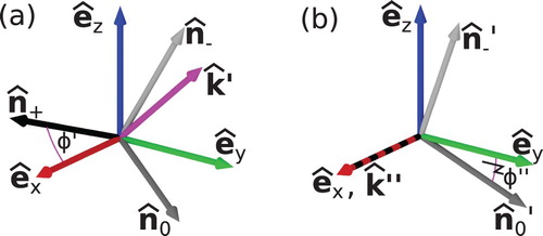19) The two consecutive rotations are illustrated by the sketch in Figure 2.

Figure 2. Sketch of the two consecutive rotations turning the orthonormal basis of instantaneous eigenvectors ${\hat{\mathit{n}}}_{+}^{\left(\alpha \right)}$, ${\hat{\mathit{n}}}_0^{\left(\alpha \right)}$, and ${\hat{\mathit{n}}}_{-}^{\left(\alpha \right)}$ into the standard basis formed by ${\hat{\mathit{e}}}_{\mathrm{x}}$, ${\hat{\mathit{e}}}_{\mathrm{y}}$, and ${\hat{\mathit{e}}}_{\mathrm{z}}$; (a) rotation of ${\hat{\mathit{n}}}_{+}^{\left(\alpha \right)}$ by the angle ${\phi }^{\mathrm{\prime }}$ around the axis ${\hat{\mathit{k}}}^{\mathrm{\prime }}$, (b) rotation of ${\hat{\mathit{n}}}_0^{\left(\alpha \right)}$ by the angle ${\phi }^{\mathrm{\prime \prime }}$ around the axis ${\hat{\mathit{k}}}^{\mathrm{\prime \prime }}$ now coinciding with ${\hat{\mathit{e}}}_{\mathrm{x}}$. After the second rotation ${\hat{\mathit{n}}}_{+}^{\left(\alpha \right)}$, ${\hat{\mathit{n}}}_0^{\left(\alpha \right)}$, and ${\hat{\mathit{n}}}_{-}^{\left(\alpha \right)}$ coincide with the vectors of the standard basis.

With these rotated mesogenic orientations, one can now compute the odf defined as (20) $\begin{array}{rl}& P_{\alpha }\left(\omega \right)\\ & =\frac{{\displaystyle \sum _{i=1}^{N_{\alpha }}⟨\left[\delta \left(\omega -{\tilde{\omega }}_i\right)+\delta \left(\omega -{\tilde{\omega }}_i^{\mathrm{\prime }}\right)\right]⟩}}{{\displaystyle {\int }_0^{2\pi }{\int }_0^{\pi }\sin \theta \mathrm{d}\theta \mathrm{d}\varphi \sum _{i=1}^{N_{\alpha }}⟨\left[\delta \left(\omega -{\tilde{\omega }}_i\right)+\delta \left(\omega -{\tilde{\omega }}_i^{\mathrm{\prime }}\right)\right]⟩}},\end{array}$(20) where δ denotes the Dirac δ-function. The ensemble averages in Equation (20(20) $\begin{array}{rl}& P_{\alpha }\left(\omega \right)\\ & =\frac{{\displaystyle \sum _{i=1}^{N_{\alpha }}⟨\left[\delta \left(\omega -{\tilde{\omega }}_i\right)+\delta \left(\omega -{\tilde{\omega }}_i^{\mathrm{\prime }}\right)\right]⟩}}{{\displaystyle {\int }_0^{2\pi }{\int }_0^{\pi }\sin \theta \mathrm{d}\theta \mathrm{d}\varphi \sum _{i=1}^{N_{\alpha }}⟨\left[\delta \left(\omega -{\tilde{\omega }}_i\right)+\delta \left(\omega -{\tilde{\omega }}_i^{\mathrm{\prime }}\right)\right]⟩}},\end{array}$(20) ) are defined through the expression (21) $\begin{array}{rl}& ⟨\delta \left(\omega -{\tilde{\omega }}_i\right)⟩\\ & =\frac{1}{Z_N}\int \mathrm{d}{\mathit{r}}^N\int \mathrm{d}{\tilde{\omega }}^N\delta \left(\omega -{\tilde{\omega }}_i\right)\exp \left[-\beta U\left({\mathit{r}}^N,{\tilde{\omega }}^N\right)\right]\\ & =\frac{1}{Z_N}\int \mathrm{d}{\tilde{\omega }}_1\dots \mathrm{d}{\tilde{\omega }}_{i-1}\mathrm{d}{\tilde{\omega }}_{i+1}\dots \mathrm{d}{\tilde{\omega }}_N\\ & \times \exp \left[-\beta U\left({\mathit{r}}^N,{\tilde{\omega }}_1,\dots {\tilde{\omega }}_{i-1},\omega ,{\tilde{\omega }}_{i+1},\dots ,{\tilde{\omega }}_N\right)\right].\end{array}$(21) In Equation (21(21) $\begin{array}{rl}& ⟨\delta \left(\omega -{\tilde{\omega }}_i\right)⟩\\ & =\frac{1}{Z_N}\int \mathrm{d}{\mathit{r}}^N\int \mathrm{d}{\tilde{\omega }}^N\delta \left(\omega -{\tilde{\omega }}_i\right)\exp \left[-\beta U\left({\mathit{r}}^N,{\tilde{\omega }}^N\right)\right]\\ & =\frac{1}{Z_N}\int \mathrm{d}{\tilde{\omega }}_1\dots \mathrm{d}{\tilde{\omega }}_{i-1}\mathrm{d}{\tilde{\omega }}_{i+1}\dots \mathrm{d}{\tilde{\omega }}_N\\ & \times \exp \left[-\beta U\left({\mathit{r}}^N,{\tilde{\omega }}_1,\dots {\tilde{\omega }}_{i-1},\omega ,{\tilde{\omega }}_{i+1},\dots ,{\tilde{\omega }}_N\right)\right].\end{array}$(21) ), (22) $Z_N=\int \mathrm{d}{\mathit{r}}^N\int \mathrm{d}{\omega }^N\exp \left[-\beta U\left({\mathit{r}}^N,{\tilde{\omega }}^N\right)\right]$(22) denotes the configuration integral, ${\mathit{r}}^N=\{{\mathit{r}}_1,{\mathit{r}}_2,\dots ,{\mathit{r}}_N\}$ and ${\tilde{\omega }}^N=\{{\tilde{\omega }}_1,{\tilde{\omega }}_2,\dots ,{\tilde{\omega }}_N\}$ represent the sets of centre-of-mass positions and orientations of the N mesogens, respectively, $\beta =1/k_{\mathrm{B}}T$ ($k_{\mathrm{B}}$ is Boltzmann's constant and T is temperature), and U is the total configurational potential energy. Because of the definition given in Equation (20(20) $\begin{array}{rl}& P_{\alpha }\left(\omega \right)\\ & =\frac{{\displaystyle \sum _{i=1}^{N_{\alpha }}⟨\left[\delta \left(\omega -{\tilde{\omega }}_i\right)+\delta \left(\omega -{\tilde{\omega }}_i^{\mathrm{\prime }}\right)\right]⟩}}{{\displaystyle {\int }_0^{2\pi }{\int }_0^{\pi }\sin \theta \mathrm{d}\theta \mathrm{d}\varphi \sum _{i=1}^{N_{\alpha }}⟨\left[\delta \left(\omega -{\tilde{\omega }}_i\right)+\delta \left(\omega -{\tilde{\omega }}_i^{\mathrm{\prime }}\right)\right]⟩}},\end{array}$(20) ), $P_{\alpha }$ is properly normalised, i.e., $\int \mathrm{d}\omega P_a\left(\omega \right)={\int }_0^{2\pi }{\int }_0^{\pi }\sin \theta \mathrm{d}\theta \mathrm{d}\varphi P_{\alpha }(\theta ,\varphi )=1$. In Equation (20(20) $\begin{array}{rl}& P_{\alpha }\left(\omega \right)\\ & =\frac{{\displaystyle \sum _{i=1}^{N_{\alpha }}⟨\left[\delta \left(\omega -{\tilde{\omega }}_i\right)+\delta \left(\omega -{\tilde{\omega }}_i^{\mathrm{\prime }}\right)\right]⟩}}{{\displaystyle {\int }_0^{2\pi }{\int }_0^{\pi }\sin \theta \mathrm{d}\theta \mathrm{d}\varphi \sum _{i=1}^{N_{\alpha }}⟨\left[\delta \left(\omega -{\tilde{\omega }}_i\right)+\delta \left(\omega -{\tilde{\omega }}_i^{\mathrm{\prime }}\right)\right]⟩}},\end{array}$(20) ), $\delta (\omega -{\tilde{\omega }}_i)$ represents $\delta (\theta -{\tilde{\theta }}_i)\delta (\varphi -{\tilde{\varphi }}_i)/\sin \theta$ and ${\tilde{\omega }}_i^{\mathrm{\prime }}=-{\tilde{\omega }}_i=(\pi -{\tilde{\theta }}_i,\pi +{\tilde{\varphi }}_i)$ to account for the head-tail symmetry (i.e., the equivalence of molecular orientations described by $\hat{\mathit{u}}$ and $-\hat{\mathit{u}}$). Moreover, it is important to notice that if component α is perfectly ordered, $P_{\alpha }=\delta \left(\varphi \right)\delta (\theta -\pi /2)$ on account of the rotation of the orientations of the mesogens which clearly satisfies the normalisation condition given above.

4. Results

4.1. Numerical details

In our current work, we employ MC simulations in the isothermal-isobaric ensemble. The thermodynamic state of the system is therefore characterised by N, the composition $x_a=1-x_b$ of the binary mixture, the pressure P, and the temperature T. Under these macroscopic constraints, the distribution of microstates in configuration space at equilibrium is proportional to $\exp [-\beta (U+PV-N{\beta }^{-1}\ln V\left)\right]$ where U is the total configurational potential energy and V is the (instantaneous) volume of the system.

We generate a Markov chain of these configurations according to the following protocol which is a properly modified version of Metropolis' original algorithm for the canonical ensemble [36]. First, it is decided with equal probability whether to displace or rotate a mesogen irrespective of the mixture component this mesogen pertains to. If a displacement is attempted, a small cube of side length δ is centred on the centre of mass of a mesogen which is then displaced randomly within the cube. The displacement is accepted (or rejected) according to the standard Metropolis criterion [36].

If instead a mesogen is to be rotated, one of the three Cartesian axes is chosen at random as the axis of rotation. Once the mesogen is rotated by a small angle increment the Metropolis criterion is again invoked to decide whether or not the rotation is accepted. Both the size of the displacement cube and the angle increment are adjusted during the course of a simulation such that about 40 – $60\mathrm{\%}$ of all attempts are accepted on average.

Once all mesogens have been selected sequentially and attempts have been made to displace or rotate them, one attempt is made to change the volume of the system by a small amount. A modified Metropolis criterion is invoked to decide whether or not this volume change is to be accepted or not [36]. Volume changes are attempted less frequently than displacement/rotation attempts because a change in volume requires in principle a recalculation of all the $N(N-1)/2$ pair contributions to U whereas during displacement/rotation events only N such interactions need to be re-evaluated.

To save as much computer time as possible, we cut off the interaction potential if the distance between the centres of mass of a pair of mesogens exceeds $3.0\sigma$. To speed up the simulations even further we employ a combination of a Verlet and linked neighbour list [37]. We consider a mesogen to be a neighbour of a reference mesogen if their centres of mass are separated by a distance of less than or equal to $3.5\sigma$.

Henceforth, we shall express all physical quantities in terms of the customary dimensionless (i.e., ‘reduced’) units. We express length in units of the diameter σ of the spherically symmetric core of the mesogens and temperature in units of $\epsilon /k_{\mathrm{B}}$ for the isotropic part of the interaction.

4.2. Nematic phases of biaxial symmetry

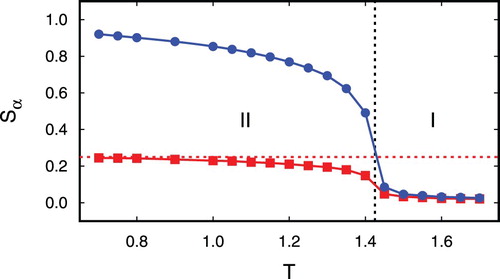
We begin the presentation of our results by displaying in Figure 3 plots of the nematic order parameters $S_{\alpha }$ for both mixture components ($\alpha =a$, b) as functions of temperature T; a plot of the biaxiality order parameter η is also shown in that figure. At sufficiently high T, $S_a\simeq S_b\simeq 0$, such that the binary mixture is globally isotropic as expected (region I). Notice, that the nematic-order parameters are not exactly zero but scale with N^(−1/2) on account of a finite-size effect that is well understood in pure liquid crystals [32,38,39].

Figure 3. Plots of the nematic-order parameters $S_{\alpha }$ as functions of temperature T for an equimolar mixture ($x_a=x_b=0.50$); the coupling strengths of the anisotropic interactions are given by ${\epsilon }_{aa}=0.050$, ${\epsilon }_{bb}=0.075$, and ${\epsilon }_{ab}=-0.150$ [see Equation (5(5) $u_{\mathrm{aniso}}^{\left(\alpha \beta \right)}\left(r_{12},{\gamma }_{12}\right)={\epsilon }_{\alpha \beta }{u}_{\mathrm{att}}\left(r_{12}\right)P_2\left(\cos {\gamma }_{12}\right),$(5) )]. The system comprises N=5000 mesogens and the simulations have been performed for a pressure P=1.00; (

) $S_a$, (

) $S_b$. In addition, the biaxiality order parameter η (

) is also shown. The dashed vertical lines demarcate zones I – III (see text); (

) $S_a=\frac{1}{4}$ (see Section 4.3).

Upon lowering T, $S_a$ and $S_b$ remain small up to $T\simeq 1.48$ when suddenly both begin to increase. This increase is stronger in the case of $\alpha =b$ compared with $\alpha =a$ (region II). As one can see, $S_b$ increases rather strongly over a small T interval and quickly assumes a relatively high value. This indicates that component b of the mixture has formed a nematic phase. The variation of $S_b$ with T appears rather rounded despite the first-order character of the isotropic-nematic phase transition. This, again, is a finite-size effect rather typical for the present class of model systems [39].

A somewhat peculiar feature is seen in the variation of $S_a$ with T. This quantity assumes a relatively small value of about 0.20 – 0.30 and increases weakly with decreasing T up to $T\simeq 1.08$ whereupon it rises rather steeply and reaches values that signal the formation of a nematic phase of component a at lower T (region III).

Compared with pure systems composed of mesogens of either component a or b the isotropic-nematic phase transition of the latter occurs at about the same $T\simeq 1.48$; the isotropic-nematic phase transition of pure component a happens at a slightly higher $T\simeq 1.13$ compared with $T\simeq 1.08$ in the binary mixture (see Figure 3).

The biaxiality order parameter η is almost zero and independent of T down to $T⪆1.10$ indicating that the partially ordered mixture is still uniaxial. For lower T, η increases steadily. This reflects that for $T\lesssim 1.10$ a biaxial nematic is forming; the biaxiality is a consequence of the increasing nematic order in component a in this range of temperatures.

That the formation of a biaxial nematic proceeds in the two-step mechanism is corroborated from ‘snapshots’ of individual configurations obtained for two thermodynamic state points pertaining to zones II and III, respectively. An inspection of Figure 4(a) indicates that mesogens of component b are predominantly aligned with the line of vision. Mesogens of component a are oriented in the plane orthogonal to the line of vision without any specific orientation. Hence, we refer to this situation as a restricted isotropic liquid component a. The normal of this plane is approximately given by the unit vector ${\hat{\mathit{n}}}_b$ of the already ordered component b. In a binary mixture of rod- and disc-like mesogens such a restricted isotropic liquid was already proposed in the work by Vanakaras et al. [26].

Figure 4. ‘Snapshots’ of individual configurations of the binary mixture (cf., Figure 3) in (a) region II (T=1.20) and (b) in region III (T=0.80), respectively. Ellipsoids of revolution pertain to component a, whereas platelets are mesogens of component b. The shape of the mesogens is exaggerated arbitrarily to improve the visibility of the orientational order in the mixture.

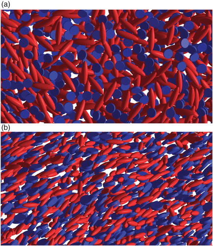
However, the ‘snapshot’ shown in Figure 4(b) clearly illustrates the biaxially symmetric nature of the mixture at the lower temperature. Mesogens of component b are still aligned with some specific direction but now mesogens of component a exhibit a preferred orientation in the plane orthogonal to that direction. It is important to note that in neither case does the binary mixture exhibit a tendency to demix.

To make sure that under the present conditions the mixture does not decompose into a- and b-rich domains we consider the local mole fractions defined as [40] (23) $\begin{array}{rl}{x}_{\alpha \alpha }\left(r_{12}\right)& =\frac{N_{\alpha \alpha }\left(r_{12}\right)}{N_{\alpha \alpha }\left(r_{12}\right)+N_{\alpha \beta }\left(r_{12}\right)},\\ & \alpha ,\beta =a,b\wedge \alpha \ne \beta ,\end{array}$(23) where (24) $N_{\alpha \beta }\left(r_{12}\right)=4\pi x_{\beta }\rho {\int }_0^{r_{12}}\mathrm{d}{\tilde{r}}_{12}{\tilde{r}}_{12}^2{g}_{\alpha \beta }\left({\tilde{r}}_{12}\right).$(24) In Equation (24(24) $N_{\alpha \beta }\left(r_{12}\right)=4\pi x_{\beta }\rho {\int }_0^{r_{12}}\mathrm{d}{\tilde{r}}_{12}{\tilde{r}}_{12}^2{g}_{\alpha \beta }\left({\tilde{r}}_{12}\right).$(24) ), $g_{\alpha \beta }$ is the radial distribution function of the centres of mass which is computed as a histogram in the usual fashion [36,37]. Plots of $g_{\alpha \beta }$ in Figure 5 reveal a couple of important features.

Figure 5. Plots of the radial pair correlation functions $g_{\alpha \beta }$ as functions of the centre-of-mass distance $r_{12}$ at a temperature T=1.00 (see Figure 3); (

) $\alpha =\beta =a$, (

) $\alpha =a$ and $\beta =b$, (

) $\alpha =\beta =b$. The inset is an enlargement around the first peak of $g_{\alpha \beta }\left(r_{12}\right)$.

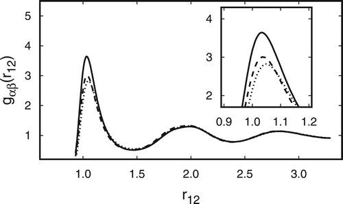
First, except for the first peak, all three radial pair correlation functions are nearly identical for $r_{12}⪆1.50$. In the first coordination shell of a reference mesogen (i.e., for $r_{12}\lesssim 1.50$), $g_{ab}$ exceeds the other two curves indicating a slightly enhanced tendency of the binary mixture to blend. Because all three radial pair correlation functions of the binary mixture are nearly the same, $N_{aa}\approx N_{ab}\approx N_{bb}$ and therefore $x_{aa}$ and $x_{bb}$ match the global composition $x_a=x_b=0.5$ except in the first coordination shell around a reference mesogen.

Second, the structure of all three radial pair correlation functions reveals the absence of long-range positional correlations as expected for a nematic phase regardless of whether it is uniaxial or biaxial. More quantitatively, we compute a correlation length $\xi \approx 3.0$ from the curves presented in Figure 5. This number is estimated by plotting the logarithm of successive maxima of $g_{\alpha \beta }$ versus the peak positions; by fitting a straight line to these data, ξ is the slope of this linear fit.

4.3. Restricted isotropic liquid

Cogitating about the data for the temperature variation of $S_a$ and η in Figure 3 a couple of important questions arise:

1. Does the increase of $S_a$ in region II signal a weakly ordered structure of component a?

2. If $S_a>0$ in region II reflects a weak orientational order, why is $\eta \simeq 0$ in regions I and II for $T⪆1.10$?

3. If the order reflected by the nonzero value of $S_a$ in region II is only ostensible, what is the orientational structure of component a in region II?

To address these questions, we further simplify our mixture by setting ${\epsilon }_{aa}=0$. Even though this situation is physically somewhat artificial, the toy model helps to elucidate the formation of biaxially ordered nematic phases in binary mixtures. In other words, interactions between a pair of mesogens of component a are purely isotropic but yet there is a certain degree of anisotropic coupling between mesogens of components a and b because ${\epsilon }_{ab}\ne 0$.

In this case, we see from plots in Figure 6 that component b undergoes an isotropic-nematic phase transition at about the same temperature $T\simeq 1.45$ observed in Figure 3 for the fully interacting system. However, this time $S_a$ increases at about this same T but then assumes a plateau value of $S_a\simeq 0.25$. No further increase of $S_a$ is observed indicating that in the idealised system component a does not form a nematic phase in line with one's physical intuition. As we have verified, in the toy model $\eta =0$ irrespective of T. Thus, we surmise that $S_a\simeq 0.25$ is most likely not indicative of a (weakly) ordered structure formed by mesogens of component a.

Figure 6. As Figure 3, but for ${\epsilon }_{aa}=0$.

To rationalise these observations let us remind the reader that ${\epsilon }_{ab}<0$ suggests that from a purely energetic perspective T-shaped arrangements of mesogens of components a and b are preferred. This also implies that if component b becomes ordered in a direction given by ${\hat{\mathit{n}}}_b$ the majority of mesogens of component a will try to avoid being oriented parallel to ${\hat{\mathit{n}}}_b$. In fact, the molecular orientations of mesogens of component a lie in a plane whose normal is more or less parallel to ${\hat{\mathit{n}}}_b$.

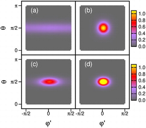
To further analyse the physical nature of the phases formed by components a and b, we present plots of $P_{\alpha }$ in Figure 7 for two thermodynamic state points in zones II and III, respectively. At T=1.20, where the corresponding plot of $S_b$ in Figure 3 indicates that component b is already in the nematic phase, the plot of $P_b$ in Figure 7(b) indicates that the odf is centred on the angles $\theta =\pi /2$ and ${\varphi }^{\mathrm{\prime }}=0$ where it has its maximum. The odf is radially symmetric and decreases fairly rapidly as a function of the ‘distance’ from its centre. The latter reflects a high degree of order in component b in agreement with the plot of $S_b$ in Figure 3.

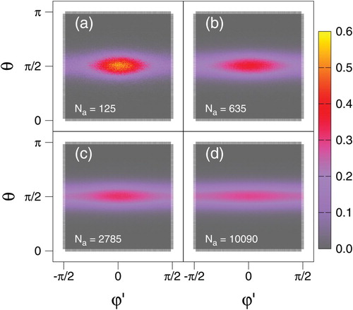
Figure 7. Plots of the orientation distribution function $P_{\alpha }\left(\omega \right)$ as functions of polar and azimuthal angles θ and ϕ. The magnitude of $P_{\alpha }$ is given by the colour bars attached to each pair of plots. Parts (a) and (c) refer to $\alpha =a$, whereas parts (b) and (d) of the figure pertain to $\alpha =b$; lower panel T=1.00, upper panel T=1.20. The higher temperature pertains to region II, whereas the lower one refers to a state point in region III in Figure 3). The azimuthal angle $\varphi ={\varphi }^{\mathrm{\prime }}+\pi$ so that $\varphi \in [0,2\pi ]$ according to its standard definition. The results in all four parts of the figure are based on simulations with N=20,000 mesogens ($x_a=0.5$).

The corresponding plot of $P_a$ in Figure 7(a) appears to be a relatively broad band centred on $\theta =\pi /2$; the band is nearly homogeneous along the ${\varphi }^{\mathrm{\prime }}$ axis at constant θ. Thus, $P_a$ characterises a nearly isotropic phase that is restricted more or less to a two-dimensional plane centred on the equator of the unit sphere mentioned in Section 3.

At T=1.00 plots in Figure 3 indicate that now the order in both components of the binary mixture is fairly substantial suggesting that now components a and b are nematic. This notion is corroborated by the plots in Figure 7(c,d). These two parts of the figure reveal that $P_a$ and $P_b$ are both centred on $\theta =\pi /2$ and ${\varphi }^{\mathrm{\prime }}=0$. The maximum of $P_b$ exceeds the one of $P_a$ which is consistent with the inequality $S_b>S_a$ that can be verified from the plots in Figure 3. Interestingly, $P_a$ and $P_b$ are no longer spherically symmetric with respect to their maxima but are elliptically deformed.

The ellipses representing $P_a$ and $P_b$ in Figure 7 are a consequence of the interaction potential between components a and b that favours a T-shaped alignment of mesogens of these two components. Hence, Figure 7(c, d) are direct evidence of the biaxiality of the globally nematic phase in region III (see Figure 3).

Therefore, the elliptic form of the odf in region III (see Figure 7) can be viewed as the analogue of the formation of the restricted isotropic phase of component a for thermodynamic states for which only component b is nematic. As mesogens of component a do not have any specific orientation in the restricted isotropic liquid, the odf of component b can still assume a spherical symmetry centred on the points ${\varphi }^{\mathrm{\prime }}=0$ and $\theta =\pi /2$ as the plots in Figure 7(a,b) clearly show.

However, it seems noteworthy that the odf in the restricted isotropic phase of component a exhibits a substantial finite-size effect. The system-size dependence of the odf is illustrated by plots in Figure 8 for various system sizes represented by the number of mesogens of component a of the mixture [at fixed composition and for the same thermodynamic state as the one for which data are shown in Figure 7(a)]. The plots in Figure 8 show that if $N_a$ is small, the odf exhibits an elliptic shape very similar to cases in which both components of the binary mixture are truly nematic [see Figure 7(c,d)]. The ellipse becomes less well defined the larger the system becomes; it vanishes completely if $N_a$ becomes sufficiently large as illustrated in Figure 7(a). In the thermodynamic limit, that is in the limit $\underset{N\to \mathrm{\infty }}{lim}\left({\lambda }_{+}^{\left(a\right)}/{\lambda }_0^{\left(a\right)}\right)=1$ (at fixed $x_a$); in any system of finite size these two eigenvalues will never be the same and the associated eigenvectors will not be degenerate.

Figure 8. As Figure 7(a), but for various system sizes indicated by the different values of $N_a$.

For completeness we demonstrate in Figure 9 that $S_a$ does not exhibit a strong finite-size effect for $N⪆5000$ [corresponding to the odf plotted in Figure 8(c)]. Noting that $S_a$ is related to an integral involving the odf, it turns out that for $N⪆5000$ a relatively small part of the odf, in which a finite-size effect is already weak, contributes to the value of $S_a$. Consequently, for these system sizes one anticipates a rather weak finite-size effect for $S_a$.

Figure 9. (a) Plots of the nematic-order parameter $S_a$ of component a in the fully interacting system as functions of the total number of mesogens N; T=1.20 (

), T=1.40 (

). (b) as (a), but in a double-logarithmic representation. The straight lines are obtained from fits assuming that $S_a-S_a^{\mathrm{\infty }}=\propto N^{{\beta }_{\mathrm{eff}}}$ where ${\beta }_{\mathrm{eff}}\approx -\frac{1}{2}$. The analysis is based upon assuming that $S_a^{\mathrm{eff}}$ can be read off part (a) of the figure for N=10000.

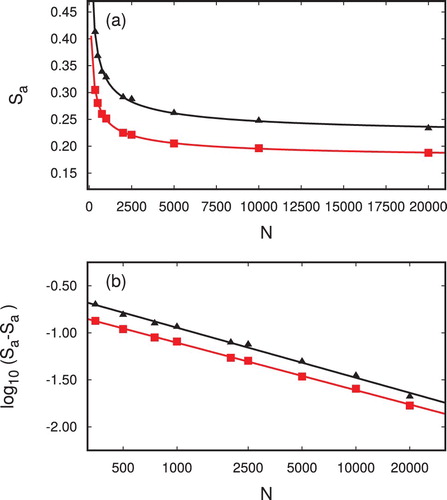
4.4. Theoretical analysis of the restricted isotropic liquid

To gain more detailed insight into the nature of the nonzero value of the nematic-order parameter of component a in the restricted isotropic liquid, we develop a simple theoretical model. Let us assume that component b is already nematic and that we take the coordinate system such that ${\hat{\mathit{n}}}_b$ coincides with the z axis. According to our above reasoning mesogens of component a will then prefer to organise themselves in the x–y plane orthogonal to the z axis. For the nematic-order parameter of component a, we adopt the alternative expression [32] (25) $S_a=\frac{1}{2N_a}⟨\sum _{i=1}^{N_a}\left(3{\cos }^2{\gamma }_i-1\right)⟩,$(25) where (26) $\cos {\gamma }_i=\hat{\mathit{u}}\left({\omega }_i\right)\cdot {\hat{\mathit{n}}}_a.$(26) The computation of $S_a$ from Equation (25(25) $S_a=\frac{1}{2N_a}⟨\sum _{i=1}^{N_a}\left(3{\cos }^2{\gamma }_i-1\right)⟩,$(25) ) is completely equivalent to the procedure based upon ${\mathbf{Q}}_a$ as was demonstrated by Eppenga and Frenkel [32]. However, the use of Equation (25(25) $S_a=\frac{1}{2N_a}⟨\sum _{i=1}^{N_a}\left(3{\cos }^2{\gamma }_i-1\right)⟩,$(25) ) tacitly assumes that ${\hat{\mathit{n}}}_a$ is both known (which is not normally the case a prior [32]) and that $\hat{\mathit{n}}\ne \mathbf{\text{0}}$. Here, we simply assume that both provisos are met.

Because of Equation (19(19) $\hat{\mathit{u}}\left({\tilde{\omega }}_i\right)={\mathbf{R}}_{\alpha }\hat{\mathit{u}}\left({\omega }_i\right),i=1,\dots ,N_{\alpha }.$(19) ), ${\hat{\mathit{n}}}_a={\hat{\mathit{e}}}_{\mathrm{x}}$. We may then rewrite the previous equation more explicitly as (27) $\cos {\gamma }_i=u_{\mathrm{x}i}=\sin {\vartheta }_i\cos {\phi }_i,$(27) using also Equation (6(6) $\widehat{\mathbf{\text{u}}}\left({\omega }_i\right)=\left(\begin{array}{c}{u}_{\mathrm{x}i}\\ u_{\mathrm{y}i}\\ u_{\mathrm{z}i}\end{array}\right)=\left(\begin{array}{c}\sin {\vartheta }_i\cos {\phi }_i\\ \sin {\vartheta }_i\sin {\phi }_i\\ \cos {\vartheta }_i\end{array}\right),i=1,2$(6) ). It is now convenient to adopt a geographical rather than the more commonly used spherical coordinate system. Accordingly, we transform coordinates such that ${\phi }_i\to {\phi }_i^{\mathrm{\prime }}={\phi }_i$ and ${\vartheta }_i\to {\vartheta }_i^{\mathrm{\prime }}={\vartheta }_i-\frac{\pi }{2}$ such that ${\phi }_i^{\mathrm{\prime }}\in [0,2\pi )$ and ${\vartheta }_i^{\mathrm{\prime }}\in [-\frac{\pi }{2},\frac{\pi }{2}]$ specify the longitude and latitude on the unit sphere, respectively. Because of this transformation we can rewrite Equation (26(26) $\cos {\gamma }_i=\hat{\mathit{u}}\left({\omega }_i\right)\cdot {\hat{\mathit{n}}}_a.$(26) ) as (28) $\cos {\gamma }_i=\sin \left({\vartheta }_i^{\mathrm{\prime }}+\pi /2\right)\cos {\phi }_i^{\mathrm{\prime }}=\cos {\vartheta }_i^{\mathrm{\prime }}\cos {\phi }_i^{\mathrm{\prime }},$(28) where we employed one of the well-known addition theorems for trigonometric functions.

Inserting the previous expression now into Equation (25(25) $S_a=\frac{1}{2N_a}⟨\sum _{i=1}^{N_a}\left(3{\cos }^2{\gamma }_i-1\right)⟩,$(25) ), the latter becomes (29) $\begin{array}{rl}{S}_a& =\frac{1}{2N_a}⟨\sum _{i=1}^{N_a}\left(3{\cos }^2{\vartheta }_i^{\mathrm{\prime }}{\cos }^2{\phi }_i^{\mathrm{\prime }}-1\right)⟩\\ & =\frac{1}{2N_a}⟨\sum _{i=1}^{N_a}\left\{\frac{3}{4}\left[1+\cos \left(2{\vartheta }_i^{\mathrm{\prime }}\right)\right]\right.\\ & \times \left.\left[1+\cos \left(2{\phi }_i^{\mathrm{\prime }}\right)\right]-1\phantom{\frac{3}{4}}\right\}\phantom{\sum _{i=1}^{N_a}}⟩,\end{array}$(29) where we have used yet another addition theorem. At this point, we introduce two new parameters, namely (30) $\begin{array}{rl}{S}_{\vartheta }& \equiv \frac{1}{N_a}⟨\sum _{i=1}^{N_a}\cos \left(2{\vartheta }_i^{\mathrm{\prime }}\right)⟩\end{array}$(30) (31) $\begin{array}{rl}{S}_{\phi }& \equiv \frac{1}{N_a}⟨\sum _{i=1}^{N_a}\cos \left(2{\phi }_i^{\mathrm{\prime }}\right)⟩.\end{array}$(31) In terms of these two parameters, Equation (29(29) $\begin{array}{rl}{S}_a& =\frac{1}{2N_a}⟨\sum _{i=1}^{N_a}\left(3{\cos }^2{\vartheta }_i^{\mathrm{\prime }}{\cos }^2{\phi }_i^{\mathrm{\prime }}-1\right)⟩\\ & =\frac{1}{2N_a}⟨\sum _{i=1}^{N_a}\left\{\frac{3}{4}\left[1+\cos \left(2{\vartheta }_i^{\mathrm{\prime }}\right)\right]\right.\\ & \times \left.\left[1+\cos \left(2{\phi }_i^{\mathrm{\prime }}\right)\right]-1\phantom{\frac{3}{4}}\right\}\phantom{\sum _{i=1}^{N_a}}⟩,\end{array}$(29) ) can then be cast as (32) $\begin{array}{rl}{S}_a& =\frac{3}{8}\left(S_{\vartheta }+S_{\phi }\right)+\frac{3}{8N_a}⟨\sum _{i=1}^{N_a}\cos \left(2{\phi }_i^{\mathrm{\prime }}\right)\cos \left(2{\vartheta }_i^{\mathrm{\prime }}\right)⟩-\frac{1}{8}\\ & \approx \frac{3}{8}\left(S_{\vartheta }+S_{\phi }+S_{\vartheta }{S}_{\phi }\right)-\frac{1}{8},\end{array}$(32) where the expression on the last line is based on the assumption that $\sum _{i=1}^{N_a}\cos \left(2{\vartheta }_i^{\mathrm{\prime }}\right)$ and $\sum _{i=1}^{N_a}\cos \left(2{\phi }_i^{\mathrm{\prime }}\right)$ are uncorrelated.

To test the robustness of this hypothesis, we introduce the covariance (33) $\begin{array}{rl}\chi & =\frac{1}{N_a}⟨\sum _{i=1}^{N_a}\cos \left(2{\phi }_i^{\mathrm{\prime }}\right)\cos \left(2{\vartheta }_i^{\mathrm{\prime }}\right)⟩\\ & -\frac{1}{N_a^2}⟨\sum _{i=1}^{N_a}\cos \left(2{\vartheta }_i^{\mathrm{\prime }}\right)⟩⟨\sum _{i=1}^{N_a}\cos \left(2{\phi }_i^{\mathrm{\prime }}\right)⟩,\end{array}$(33) where the ensemble averages are computed from the expression (34) $\begin{array}{rl}& \frac{1}{N_a}⟨\sum _{i=1}^{N_a}\left\{\begin{array}{c}\cos \left(2{\phi }_i^{\mathrm{\prime }}\right)\cos \left(2{\vartheta }_i^{\mathrm{\prime }}\right)\\ \cos \left(2{\vartheta }_i^{\mathrm{\prime }}\right)\\ \cos \left(2{\phi }_i^{\mathrm{\prime }}\right)\end{array}\right.⟩\\ & ={\int }_0^{2\pi }{\int }_{-\pi /2}^{\pi /2}\left.\begin{array}{c}\cos \left(2{\phi }^{\mathrm{\prime }}\right)\cos \left(2{\vartheta }^{\mathrm{\prime }}\right)\\ \cos \left(2{\vartheta }^{\mathrm{\prime }}\right)\\ \cos \left(2{\phi }^{\mathrm{\prime }}\right)\end{array}\right\}{P}_a\left({\vartheta }^{\mathrm{\prime }},{\phi }^{\mathrm{\prime }}\right)\\ & \times \cos {\vartheta }^{\mathrm{\prime }}\mathrm{d}{\vartheta }^{\mathrm{\prime }}\mathrm{d}{\phi }^{\mathrm{\prime }}.\end{array}$(34) Here, $\cos {\vartheta }^{\mathrm{\prime }}$ is the Jacobian determinant for the transformation from Cartesian to geographical coordinates. 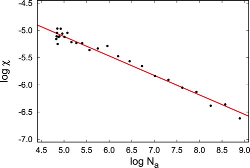In the above expressions, $P_a$ is taken from MC simulations for the fully interacting system. It is apparent from Figure 10 that indeed χ is a very small quantity indicating that the correlation between $\sum _{i=1}^{N_a}\cos \left(2{\vartheta }_i^{\mathrm{\prime }}\right)$ and $\sum _{i=1}^{N_a}\cos \left(2{\phi }_i^{\mathrm{\prime }}\right)$ is very small. Figure 10 also shows that the approximation becomes even better for larger system sizes but is already very good for the smallest ones considered.

Figure 10. Double logarithmic plot of the covariance defined in Equation (33(33) $\begin{array}{rl}\chi & =\frac{1}{N_a}⟨\sum _{i=1}^{N_a}\cos \left(2{\phi }_i^{\mathrm{\prime }}\right)\cos \left(2{\vartheta }_i^{\mathrm{\prime }}\right)⟩\\ & -\frac{1}{N_a^2}⟨\sum _{i=1}^{N_a}\cos \left(2{\vartheta }_i^{\mathrm{\prime }}\right)⟩⟨\sum _{i=1}^{N_a}\cos \left(2{\phi }_i^{\mathrm{\prime }}\right)⟩,\end{array}$(33) ) as a function of the number of particles of component a. Data are shown for T=1.40 pertaining to region II (see Figure 3). The symbols represent MC results and the continuous line is a fit to these data intended to guide the eye.

Let us now assume that the orientations of mesogens of component a are completely restricted to the x–y plane. In other words, ${\vartheta }_i$ is zero irrespective of i and therefore $S_{\vartheta }=1$ [see Equation (30(30) $\begin{array}{rl}{S}_{\vartheta }& \equiv \frac{1}{N_a}⟨\sum _{i=1}^{N_a}\cos \left(2{\vartheta }_i^{\mathrm{\prime }}\right)⟩\end{array}$(30) )]. In this case, Equation (32(32) $\begin{array}{rl}{S}_a& =\frac{3}{8}\left(S_{\vartheta }+S_{\phi }\right)+\frac{3}{8N_a}⟨\sum _{i=1}^{N_a}\cos \left(2{\phi }_i^{\mathrm{\prime }}\right)\cos \left(2{\vartheta }_i^{\mathrm{\prime }}\right)⟩-\frac{1}{8}\\ & \approx \frac{3}{8}\left(S_{\vartheta }+S_{\phi }+S_{\vartheta }{S}_{\phi }\right)-\frac{1}{8},\end{array}$(32) ) reduces to the expression (35) $S_a=\frac{1}{4}+\frac{3}{4}{S}_{\phi },$(35) where now $S_{\phi }$ is the two-dimensional nematic-order parameter evaluated by Frenkel and Eppenga [41]. If this two-dimensional system is isotropic, $P_a=1/2\pi \delta \left({\vartheta }^{\mathrm{\prime }}\right)$ such that (36) $\begin{array}{rl}{S}_{\phi }& ={\int }_0^{2\pi }{\int }_{-\pi /2}^{\pi /2}\cos \left(2{\phi }^{\mathrm{\prime }}\right)\cos {\vartheta }^{\mathrm{\prime }}{P}_a\left({\vartheta }^{\mathrm{\prime }},{\phi }^{\mathrm{\prime }}\right)\mathrm{d}{\vartheta }^{\mathrm{\prime }}\mathrm{d}{\phi }^{\mathrm{\prime }}\\ & =\frac{1}{2\pi }{\int }_0^{2\pi }\cos \left(2{\phi }^{\mathrm{\prime }}\right)\mathrm{d}{\phi }^{\mathrm{\prime }}=0\end{array}$(36) and the expression in Equation (35(35) $S_a=\frac{1}{4}+\frac{3}{4}{S}_{\phi },$(35) ) reduces to a constant $S_a=\frac{1}{4}$. For the toy model, it is clear from the plot of $S_a$ in Figure 6 that the threshold value of $\frac{1}{4}$ is appoached at sufficiently low T in region II. Similarly, $S_a=\frac{1}{4}$ is reached at $T\simeq 1.32$ in the fully interacting system as the relevant plot in Figure 3 illustrates.

But why does $S_a$ approach the threshold value of $\frac{1}{4}$ from below for both the toy and fully interacting models? Based upon the plot in Figure 7(a) one realises that the assumption of a strictly two-dimensional arrangement of mesogens of component a is too strong. Apparently, some molecules have orientations that are characterised by angles ${\vartheta }^{\mathrm{\prime }}$ slightly smaller or larger than $\pi /2$ (corresponding to ${\vartheta }^{\mathrm{\prime }}$ slightly smaller or larger than zero). In turn, $S_{\vartheta }<1$.

To account for this reduction in a bit more quantitative fashion, we introduce $S_{\vartheta }=1-ϵ$ where ε is a small, temperature dependent quantity. A lucid interpretation of ε is that of the variance of $P_a$ at constant ${\phi }^{\mathrm{\prime }}$ and variable ${\vartheta }^{\mathrm{\prime }}$ [see Figure 7(a)]. It is therefore plausible to expect $ϵ\to 0$ with decreasing T. This is because as T decreases, mesogens of component a are suffering an increasing loss in kinetic energy. This prevents them to an increasing degree from overcoming the energy penalty associated with aligning more with the z axis.

We are therefore in a postion to replace $S_{\vartheta }$ on the second line of Equation (29(29) $\begin{array}{rl}{S}_a& =\frac{1}{2N_a}⟨\sum _{i=1}^{N_a}\left(3{\cos }^2{\vartheta }_i^{\mathrm{\prime }}{\cos }^2{\phi }_i^{\mathrm{\prime }}-1\right)⟩\\ & =\frac{1}{2N_a}⟨\sum _{i=1}^{N_a}\left\{\frac{3}{4}\left[1+\cos \left(2{\vartheta }_i^{\mathrm{\prime }}\right)\right]\right.\\ & \times \left.\left[1+\cos \left(2{\phi }_i^{\mathrm{\prime }}\right)\right]-1\phantom{\frac{3}{4}}\right\}\phantom{\sum _{i=1}^{N_a}}⟩,\end{array}$(29) ) by $1-ϵ$ which yields (37) $S_a=\frac{1}{4}+\left(\frac{3}{4}-\frac{3}{8}ϵ\left(T\right)\right)S_{\phi }-\frac{3}{8}ϵ\left(T\right).$(37) If we now assume that the distribution of the $\left\{{\phi }_i^{\mathrm{\prime }}\right\}$ is isotropic Equation (37) reduces to $S_a=\frac{1}{4}-\frac{3}{8}ϵ\le \frac{1}{4}$ which indicates that if component a is not completely restricted to the x–y plane there will be a negative deviation of $S_a$ from the ideal two-dimensional threshold value and this is the reason for why the threshold value of $S_a=\frac{1}{4}$ in Figure 6; the deviation becomes smaller as T decreases.

The situation is a bit different for the fully interacting system because the relevant plot in Figure 3 reveals that for sufficiently low T, $S_a$ can also exceed the theoretical threshold value of $\frac{1}{4}$. This can be explained as follows.

Because in the fully interacting system the mesogens can align in principle, $S_{\phi }$ is not necessarily zero everywhere in region II and increases further with decreasing T. This notion is supported by the plot of $S_{\phi }$ in Figure 11. However, it is conceivable that for sufficiently high T in region II, $S_{\phi }$ is still small enough so that the third term on the righthand side of Equation (37(37) $S_a=\frac{1}{4}+\left(\frac{3}{4}-\frac{3}{8}ϵ\left(T\right)\right)S_{\phi }-\frac{3}{8}ϵ\left(T\right).$(37) ) outweighs the second one. Consequently, $S_a<\frac{1}{4}$ in this temperature range. Because ε decreases but $S_{\phi }$ increases (see Figure 11) with decreasing T, one can envision that at $T\simeq 1.32$ the two terms cancel exactly such that $S_a=\frac{1}{4}$. For even lower T the second term is always more significant energetically such that $S_a>\frac{1}{4}$ until eventually component a undergoes an isotropic nematic phase transition.

Figure 11. As Fig. 3, but for $S_{\phi }$ (

) and (

), and for $S_{\vartheta }$ (

) and (

). Dashed vertical lines are estimates of the temperatures for the phase transitions from isotropic to uniaxial nematic ($T\simeq 1.48$) and from uniaxial to biaxial nematic phases ($T\simeq 1.08$). The horizontal dashed line (

) corresponds to the threshold value $S_a=\frac{1}{4}$, while (

) refers to $S_{\vartheta }=\frac{1}{3}$ [see Equation 38(38) $\begin{array}{rl}{S}_{\vartheta }& ={\int }_0^{2\pi }{\int }_{-\pi /2}^{\pi /2}\cos \left(2{\vartheta }^{\mathrm{\prime }}\right)P_a\left({\vartheta }^{\mathrm{\prime }},{\phi }^{\mathrm{\prime }}\right)\cos {\vartheta }^{\mathrm{\prime }}\mathrm{d}{\vartheta }^{\mathrm{\prime }}\mathrm{d}{\phi }^{\mathrm{\prime }}\\ & =\frac{1}{2}{\int }_{-\pi /2}^{\pi /2}\cos \left(2{\vartheta }^{\mathrm{\prime }}\right)\cos {\vartheta }^{\mathrm{\prime }}\mathrm{d}{\vartheta }^{\mathrm{\prime }}=\frac{1}{3},\end{array}$(38) ]. Data for $S_a$ (

) and (

) are shown for comparison. Open and filled symbols refer to cooling and heating runs, respectively (see text). In all cases, data are obtained for systems comprising N=5000 mesogens (cf., Figure 9).

The plot of $S_{\vartheta }$ in Figure 11 indicates that this quantity is about $\frac{1}{3}$ for temperatures where both components are isotropic. This value is easy to understand because in the completely isotropic phase (region I), $S_{\vartheta }$ can be calculated analytically from the expression (38) $\begin{array}{rl}{S}_{\vartheta }& ={\int }_0^{2\pi }{\int }_{-\pi /2}^{\pi /2}\cos \left(2{\vartheta }^{\mathrm{\prime }}\right)P_a\left({\vartheta }^{\mathrm{\prime }},{\phi }^{\mathrm{\prime }}\right)\cos {\vartheta }^{\mathrm{\prime }}\mathrm{d}{\vartheta }^{\mathrm{\prime }}\mathrm{d}{\phi }^{\mathrm{\prime }}\\ & =\frac{1}{2}{\int }_{-\pi /2}^{\pi /2}\cos \left(2{\vartheta }^{\mathrm{\prime }}\right)\cos {\vartheta }^{\mathrm{\prime }}\mathrm{d}{\vartheta }^{\mathrm{\prime }}=\frac{1}{3},\end{array}$(38) where we employed the fact that in the isotropic phase in region I, $P_a=1/4\pi$. However, in any system of finite size, $S_{\vartheta }$ exceeds the value of $\frac{1}{3}$ slightly. At $T\simeq 1.48$, $S_{\vartheta }$ rises steeply. This is the same temperature at which component b becomes nematic (see Figure 3). This is not surprising either because an increase in $S_{\vartheta }$ signals the onset of the formation of the restricted isotropic liquid component a.

In Figure 11 we show two sets of data for each of the three quantities plotted. We computed $S_{\vartheta }$ and $S_{\varphi }$ from Equations (30(30) $\begin{array}{rl}{S}_{\vartheta }& \equiv \frac{1}{N_a}⟨\sum _{i=1}^{N_a}\cos \left(2{\vartheta }_i^{\mathrm{\prime }}\right)⟩\end{array}$(30) ), (31(31) $\begin{array}{rl}{S}_{\phi }& \equiv \frac{1}{N_a}⟨\sum _{i=1}^{N_a}\cos \left(2{\phi }_i^{\mathrm{\prime }}\right)⟩.\end{array}$(31) ), and (34(34) $\begin{array}{rl}& \frac{1}{N_a}⟨\sum _{i=1}^{N_a}\left\{\begin{array}{c}\cos \left(2{\phi }_i^{\mathrm{\prime }}\right)\cos \left(2{\vartheta }_i^{\mathrm{\prime }}\right)\\ \cos \left(2{\vartheta }_i^{\mathrm{\prime }}\right)\\ \cos \left(2{\phi }_i^{\mathrm{\prime }}\right)\end{array}\right.⟩\\ & ={\int }_0^{2\pi }{\int }_{-\pi /2}^{\pi /2}\left.\begin{array}{c}\cos \left(2{\phi }^{\mathrm{\prime }}\right)\cos \left(2{\vartheta }^{\mathrm{\prime }}\right)\\ \cos \left(2{\vartheta }^{\mathrm{\prime }}\right)\\ \cos \left(2{\phi }^{\mathrm{\prime }}\right)\end{array}\right\}{P}_a\left({\vartheta }^{\mathrm{\prime }},{\phi }^{\mathrm{\prime }}\right)\\ & \times \cos {\vartheta }^{\mathrm{\prime }}\mathrm{d}{\vartheta }^{\mathrm{\prime }}\mathrm{d}{\phi }^{\mathrm{\prime }}.\end{array}$(34) ); $S_a$ is computed from Equation (32(32) $\begin{array}{rl}{S}_a& =\frac{3}{8}\left(S_{\vartheta }+S_{\phi }\right)+\frac{3}{8N_a}⟨\sum _{i=1}^{N_a}\cos \left(2{\phi }_i^{\mathrm{\prime }}\right)\cos \left(2{\vartheta }_i^{\mathrm{\prime }}\right)⟩-\frac{1}{8}\\ & \approx \frac{3}{8}\left(S_{\vartheta }+S_{\phi }+S_{\vartheta }{S}_{\phi }\right)-\frac{1}{8},\end{array}$(32) ). Both sets in Fig 11 are obtained from restart runs in which T between successive restarts is lowered (cooling sequence) or raised (heating sequence). No significant difference between cooling and heating is detected. Thus, because of the absence of hysteresis in the plots of Figure 11, the formation of a uniaxial and a biaxial nematic phase appears to be a continuous rather than a first-order phase transitions.

However, for this class of models of nematic liquid crystals it has been established that the isotropic-nematic phase transition is very weakly first-order and that it follows a true discontinuous phase transition. This was demonstrated by Greschek [35] and by Greschek and Schoen a while ago who used concepts of finite-size scaling [39]; it was also demonstrated in a more recent density-functional study of a pure nematic liquid crystal also pertaining to the present class of model systems [30]. The reason for this very weak first-order phase transition is perhaps the spherically symmetric isotropic core of the mesogens.

5. Discussion and conclusion

In our work, we focus on binary mixtures of two liquid-crystalline compounds that are capable of forming nematic phases under favourable thermodynamic conditions. For each separate pure component, the orientation dependence of the anisotropic interactions is that of the well-known Maier-Saupe model. That is, for a fixed relative orientation of a pair of mesogens, the potential is isotropic and hence does not depend on the orientation of the distance vector connecting the centres of mass of the mesogens. If the coupling constant governing the anisotropic interactions is positive, a side-by-side arrangement of the mesogens (i.e., an angle of 0 or π between the unit vectors describing the orientations of the mesogens) is energetically the most favourable. Thus, if the pure components become nematic, these nematic phases have uniaxial symmetry.

For the interaction between the different components of the mixture, we maintain the Maier-Saupe orientation dependence but with a negative instead of a positive coupling constant. This way the different mesogens of the mixture prefer a T-shaped relative orientation. If the magnitude of the coupling constant is not made too small the demixing of the mixture into larger domains, in which mostly mesogens of one or the other component are found, is suppressed. This is advantageous because it enables us to study the formation of biaxial phases without having to deal with an accompanying demixing process that would be superimposed on the formation of a biaxially ordered phase and blur it.

For suitably chosen coupling constants ${\epsilon }_{aa}<{\epsilon }_{bb}$ (${\epsilon }_{aa}>0$) and ${\epsilon }_{ab}<0$ the formation of a biaxially ordered nematic phase is found to be a two-step process. Under these conditions and for a sufficiently low T, component b first forms a nematic structure of uniaxial symmetry. When this happens, the nematic-order parameter $S_a$ of component a increases by a fair amount which may seem puzzling because the value assumed $S_a\simeq 0.25$ is hardly large enough to indicate the formation of a nematic phase in component a as well. Even more puzzling is the fact that the biaxiality of the entire liquid crystal is close to zero indicating that no biaxially ordered phase has formed.

To understand these seemingly enigmatic observations, we analyse an idealised (toy) system in which mesogens of component a can be oriented but remain disordered because we set ${\epsilon }_{aa}=0$. Because there cannot be any correlation between orientations of mesogens of component a in our toy model, one can completely neglect the correlations between the orientations of the different mesogens of component a. However, a perfect restriction of these orientations to two dimensions will not happen in reality on account of thermal fluctuations. Within the framework of a simple theoretical approach, we are able to rationalise the threshold value of $S_a=\frac{1}{4}$, which is approached from below in the toy model, because of these thermal fluctuations.

In the fully interacting system, $S_a$ can be smaller or larger than the threshold value of $\frac{1}{4}$. This is because there are two contributions that counterbalance each other. The first is the nematic order parameter $S_{\phi }$ of the quasi-two-dimensional restricted phase and the variance of the odf at fixed azimuthal and variable out-of-plane (i.e., polar) angle. Whereas the first parameter tends to increase as T goes down, the variance of the odf decreases as the mesogens loose kinetic energy.

It should, however, be borne in mind that the nonzero value of $S_a$ is a consequence of the restriction of an isotropic liquid to a two-dimensional plane; neither does it indicate any nematic order nor does it reflect biaxiality in the sense of S and η which are defined for the mixture as a whole. In this sense, $S_a$ and ${\eta }_a$ reflect only that the original, three-dimensional isotropic liquid formed by component a (region I, see Figures 3 and 6) is suddenly forced to become quasi two-dimensional but remains isotropic while component b undergoes an isotropic-nematic transition.

Another quantity that we analyse in depth is a two-dimensional odf. To compute this odf with sufficient resolution and accuracy, it is advantageous to rotate the instantaneous eigensystem of ${\mathbf{Q}}_{\alpha }$ such that the eigenvector corresponding to the nematic order parameter (i.e., the largest one) always coincides with the x axis, say. Using such an instantaneous coordinate system rather than a space-fixed one is particularly benefitial in smaller systems in which the nematic director can exhibit a slow but permanent reorientation over the course of a simulation.

The odf gives clear evidence of the two-step process during which a globally nematic phase of biaxial symmetry forms and of the existence of an intermittent restricted isotropic liquid phase of component a. When this restricted isotropic liquid is stable but component b is already in the uniaxially symmetric nematic phase the odf of component a turns out to be a strip-like ‘cloud’ centred on the polar angle $\theta =\pi /2$ and independent of the azimuthal angle ${\varphi }^{\mathrm{\prime }}$; because phase b is embedded in this restricted isotropic liquid its odf is spherically symmetric and rather peaked at the angles $\theta =\pi /2$ and ${\varphi }^{\mathrm{\prime }}=0$.

If this novel restricted isotropic liquid phase finally becomes ordered as well (and when the global symmetry of the liquid crystal mixture is biaxial) the odf of both components is elliptically deformed. This is a consequence of the interaction potential because orientations of mesogens that are favourable for mesogens of one component are unfavourable for the other one and vice versa. It is this feature of our model that is ultimately responsible for the elliptic deformation of the odf of both components when a biaxially symmetric phase forms.

Disclosure statement

No potential conflict of interest was reported by the authors.

ORCID

George Jackson  http://orcid.org/0000-0002-8029-8868

Additional information

Funding

Three of us (L. L., S. P.-S., and M. S.) are grateful to the Deutsche Forschungsgemeinschaft for financial support within the International Graduate Research Training Group 1524. Support from the Engineering and Physical Sciences Research Council (EPSRC) of the UK to the Molecular Systems Engineering group at Imperial College London through Grants EP/EP016340 and EP/J014958 is gratefully acknowledged.

Appendix. Construction of the rotation tensor

To determine the orientation distribution function, we argue in Section 3 that the orientation of the mesogens is best analysed in a frame of reference spanned by the eigenvectors of ${\mathbf{Q}}_{\alpha }$. Because the orientations of the mesogens $\left\{{\hat{\mathit{u}}}_i\right\}$ are given in a space-fixed frame of reference that remains the same throughout the simulation, the analysis in the eigenvector frame of reference requires a rotation of the individual orientations of the mesogens between successive configurations.

In general and guided by the principles of linear algebra, a transformation of a (unit) vector $\hat{\mathit{a}}$ given in one frame of reference to its counterpart $\hat{\mathit{b}}$ in another such frame is effected by the equation (A1) $\hat{\mathit{b}}=\mathbf{R}(\hat{\mathit{k}},\phi )\hat{\mathit{a}},$(A1) where φ is the angle of rotation about an axis $\stackrel{\mathbf{ˆ}}{\mathbf{k}}$ defined by (A2) $\hat{\mathit{k}}=\frac{\hat{\mathit{a}}\times \hat{\mathit{b}}}{\parallel \hat{\mathit{a}}\times \hat{\mathit{b}}\parallel },$(A2) and $\parallel \dots \parallel$ is the vector norm. The rotation tensor $\mathbf{R}$ in Equation (A1(A1) $\hat{\mathit{b}}=\mathbf{R}(\hat{\mathit{k}},\phi )\hat{\mathit{a}},$(A1) ) satisfies ${\mathbf{R}}^{\mathrm{T}}={\mathbf{R}}^{-1}$ such that $\mathbf{R}{\mathbf{R}}^{\mathrm{T}}=\mathbf{1}$. In addition, $\det \mathbf{R}=1$ where ‘$\det$’ indicates the determinant. Because we are working in three-dimensional space, $\mathbf{R}$ is a second-rank tensor that can be represented by a $3\times 3$ matrix.

An alternative version of Equation (A1(A1) $\hat{\mathit{b}}=\mathbf{R}(\hat{\mathit{k}},\phi )\hat{\mathit{a}},$(A1) ) is given by the so-called Euler-Rodrigues equation [42] which states that (A3) $\hat{\mathit{b}}=\hat{\mathit{a}}+2q_0\mathit{q}\times \hat{\mathit{a}}+2\mathit{q}\times \left(\mathit{q}\times \hat{\mathit{a}}\right),$(A3) where $(q_0,\mathit{q})$ is a four-dimensional vector known as a quaternion first introduced into classical mechanics by Hamilton [43]; the scalar $q_0$ and the vector ${\mathit{q}}^{\mathrm{T}}=(q_1,q_2,q_3)$ are given by the expressions (A4a) $\begin{array}{rl}{q}_0& =\cos \left(\frac{\phi }{2}\right)\end{array}$(A4a) (A4b) $\begin{array}{rl}\mathit{q}& =\hat{\mathit{k}}\sin \left(\frac{\phi }{2}\right).\end{array}$(A4b) The angle of rotation is obtained from the expression (A5) $\cos \phi =\hat{\mathit{a}}\cdot \hat{\mathit{b}}.$(A5) Inserting Equations (A4a(A4a) $\begin{array}{rl}{q}_0& =\cos \left(\frac{\phi }{2}\right)\end{array}$(A4a) ) and (A4b(A4b) $\begin{array}{rl}\mathit{q}& =\hat{\mathit{k}}\sin \left(\frac{\phi }{2}\right).\end{array}$(A4b) ) into Equation (A3(A3) $\hat{\mathit{b}}=\hat{\mathit{a}}+2q_0\mathit{q}\times \hat{\mathit{a}}+2\mathit{q}\times \left(\mathit{q}\times \hat{\mathit{a}}\right),$(A3) ) allows us to rewrite the latter as (A6) $\begin{array}{rl}\hat{\mathit{b}}& =\hat{\mathit{a}}+2\cos \left(\frac{\phi }{2}\right)\sin \left(\frac{\phi }{2}\right)\hat{\mathit{k}}\times \hat{\mathit{a}}\\ & +2{\sin }^2\left(\frac{\phi }{2}\right)\hat{\mathit{k}}\times \left(\hat{\mathit{k}}\times \hat{\mathit{a}}\right)\\ & =\left[\mathbf{1}+\mathbf{K}\sin \phi +{\mathbf{K}}^2\left(1-\cos \phi \right)\right]\hat{\mathit{a}},\end{array}$(A6) where we used the well-known textbook expressions for trigonometric functions of half-angle arguments and $\mathbf{K}$ is given by the traceless skew-symmetric tensor (A7) $\begin{array}{r}\mathbf{K}=\left(\begin{array}{ccc}0& -k_3& k_2\\ k_3& 0& -k_1\\ -k_2& k_1& 0\end{array}\right)\end{array}$(A7) of components of $\hat{\mathit{k}}$. Because of this form of $\mathbf{K}$ and because $\parallel \hat{\mathit{k}}\parallel =1$, it follows that (A8) ${\mathbf{K}}^2=-\mathbf{1}+\hat{\mathit{k}}\otimes \hat{\mathit{k}}.$(A8) With this expression, it is easy to see that Equation (A6(A9) $\begin{array}{rl}\hat{\mathit{b}}& =(\mathbf{K}\sin \phi +\mathbf{1}\cos \phi +\hat{\mathit{k}}\otimes \hat{\mathit{k}})\hat{\mathit{a}}\\ & =(\mathbf{K}\sin \phi +\mathbf{1}\cos \phi )\hat{\mathit{a}}+(\hat{\mathit{k}}\cdot \hat{\mathit{a}})\hat{\mathit{k}}\\ & =\left(\mathbf{K}\sin \phi +\mathbf{1}\cos \phi \right)\hat{\mathit{a}},\end{array}$(A9) ) can be recast as (A9) $\begin{array}{rl}\hat{\mathit{b}}& =(\mathbf{K}\sin \phi +\mathbf{1}\cos \phi +\hat{\mathit{k}}\otimes \hat{\mathit{k}})\hat{\mathit{a}}\\ & =(\mathbf{K}\sin \phi +\mathbf{1}\cos \phi )\hat{\mathit{a}}+(\hat{\mathit{k}}\cdot \hat{\mathit{a}})\hat{\mathit{k}}\\ & =\left(\mathbf{K}\sin \phi +\mathbf{1}\cos \phi \right)\hat{\mathit{a}},\end{array}$(A9) where we have used the identity $(\hat{\mathit{k}}\otimes \hat{\mathit{k}})\hat{\mathit{a}}=(\hat{\mathit{k}}\cdot \hat{\mathit{a}})\hat{\mathit{k}}$ that is also easy to prove. The last line of the previous expression follows because $\hat{\mathit{k}}\cdot \hat{\mathit{a}}=0$. This is clear from Equation (A2(A2) $\hat{\mathit{k}}=\frac{\hat{\mathit{a}}\times \hat{\mathit{b}}}{\parallel \hat{\mathit{a}}\times \hat{\mathit{b}}\parallel },$(A2) ) because the rotation axis is always orthogonal to the vector $\hat{\mathit{a}}$. Thus, by comparison with Equation (A1(A1) $\hat{\mathit{b}}=\mathbf{R}(\hat{\mathit{k}},\phi )\hat{\mathit{a}},$(A1) ), one realises that (A10) $\mathbf{R}(\hat{\mathit{k}},\phi )=\mathbf{K}\sin \phi +\mathbf{1}\cos \phi .$(A10) As a brief demonstration of the validity of Equation (A10(A10) $\mathbf{R}(\hat{\mathit{k}},\phi )=\mathbf{K}\sin \phi +\mathbf{1}\cos \phi .$(A10) ), let us consider two special cases. In the first of these, we take $\phi =0$ and therefore $\mathbf{R}=\mathbf{1}$. From Equation (A10(A10) $\mathbf{R}(\hat{\mathit{k}},\phi )=\mathbf{K}\sin \phi +\mathbf{1}\cos \phi .$(A10) ), we readily obtain $\hat{\mathit{b}}=\hat{\mathit{a}}$, that is the ‘rotation’ leaves the vector $\hat{\mathit{a}}$ unchanged. In the second case, we take the angle of rotation to be given by $\phi =\pi$. Again, from Equation (A10(A10) $\mathbf{R}(\hat{\mathit{k}},\phi )=\mathbf{K}\sin \phi +\mathbf{1}\cos \phi .$(A10) ), it is easy to see that now $\mathbf{R}=-\mathbf{1}$ and therefore $\hat{\mathit{b}}=-\hat{\mathit{a}}$. Thus, in this case the vector $\stackrel{\mathbf{ˆ}}{\mathbf{a}}$ suffers its inversion by the application of the tensor $\mathbf{R}$ as it should. Notice, that in both cases, the specific axis of rotation does not matter because $\sin \phi =0$ in Equation (A10(A10) $\mathbf{R}(\hat{\mathit{k}},\phi )=\mathbf{K}\sin \phi +\mathbf{1}\cos \phi .$(A10) ). In fact, $\hat{\mathit{k}}$ is even undefined because $\hat{\mathit{a}}\times r\hat{\mathit{a}}=\mathbf{\text{0}}$ in Equation (A2(A2) $\hat{\mathit{k}}=\frac{\hat{\mathit{a}}\times \hat{\mathit{b}}}{\parallel \hat{\mathit{a}}\times \hat{\mathit{b}}\parallel },$(A2) ) for any number $r\in \mathbb{R}$ and therefore the norm in the denominator of the expression on the righthand side of Equation (A2(A2) $\hat{\mathit{k}}=\frac{\hat{\mathit{a}}\times \hat{\mathit{b}}}{\parallel \hat{\mathit{a}}\times \hat{\mathit{b}}\parallel },$(A2) ) would vanish as well. Another interpretation of this observation is that an infinite manifold of axes $\hat{\mathit{k}}$ exists that can be employed to invert a vector by rotation.

References

- P.H. Poole, T. Grande, C.A. Angell and P.F. McMillan, Science 275, 322–323 (1997). doi: 10.1126/science.275.5298.322
- T. Kato, Science 295, 2414–2418 (2002). doi: 10.1126/science.1070967
- P.G. de Gennes and J. Prost, The Physics of Liquid Crystals 2nd ed. (Oxford University Press, Oxford, 1995).
- F. Reinitzer, Monatsh. Chem. 9, 421–441 (1888). doi: 10.1007/BF01516710
- O. Lehmann, Z. Phys. Chem. 4, 462–472 (1889).
- A.V. Kityk, M. Wolff, K. Knorr, D. Morineau, R. Lefort and P. Huber, Phys. Rev. Lett. 101, 187801 (2008). doi: 10.1103/PhysRevLett.101.187801
- M.J. Freiser, Phys. Rev. Lett. 24, 1041–1043 (1970). doi: 10.1103/PhysRevLett.24.1041
- G.R. Luckhurst, Thin Solid Films 393, 40–52 (2001). doi: 10.1016/S0040-6090(01)01091-4
- G.R. Luckhurst, Nature 430 (6998), 413–414 (2004). doi: 10.1038/430413a
- L.A. Madsen, T.J. Dingemans, M. Nakata and E.T. Samulski, Phys. Rev. Lett. 92, 145505 (2004).
- J.J. Hunt, R.W. Date, B.A. Timimi, G.R. Luckhurst and D.W. Bruce, J. Am. Chem. Soc. 123, 10115–10116 (2001). doi: 10.1021/ja015943q
- T. Hegmann, J. Kain, S. Diele, G. Pelzl and C. Tschierske, Angew. Chemie 113, 911–914 (2001). doi: 10.1002/1521-3757(20010302)113:5<911::AID-ANGE911>3.0.CO;2-S
- L.J. Yu and A. Saupe, Phys. Rev. Lett. 45, 1000–1003 (1980). doi: 10.1103/PhysRevLett.45.1000
- E.A. Oliveira, L. Liebert and A.M. Figueiredo Neto, Liq. Cryst. 5, 1669–1675 (1989). doi: 10.1080/02678298908045677
- R. Berardi and C. Zannoni, J. Chem. Phys. 113, 5971–5979 (2000). doi: 10.1063/1.1290474
- P.J. Camp and M.P. Allen, J. Chem. Phys. 106, 6681–6688 (1997). doi: 10.1063/1.473665
- A.G. Vanakaras, M.A. Bates and D.J. Photinos, Phys. Chem. Chem. Phys. 5, 3700–3706 (2003). doi: 10.1039/b306271f
- R. Alben, J. Chem. Phys. 59, 4299–4304 (1973). doi: 10.1063/1.1680625
- A. Stroobants and H.N.W. Lekkerkerker, J. Phys. Chem. 88, 3669–3674 (1984). doi: 10.1021/j150660a058
- H.H. Wensink, G.J. Vroege and H.N.W. Lekkerkerker, Phys. Rev. E 66, 041704 (2002). doi: 10.1103/PhysRevE.66.041704
- S.R. Sharma, P. Palffy-Muhoray, B. Bergersen and D.A. Dunmur, Phys. Rev. A 32, 3752–3755 (1985). doi: 10.1103/PhysRevA.32.3752
- J. Delhommelle and P. Millié, Mol. Phys. 99, 619–625 (2001). doi: 10.1080/00268970010020041
- P. Palffy-Muhoray, J.R. de Bruyn and D.A. Dunmur, J. Chem. Phys. 82, 5294–5295 (1985). doi: 10.1063/1.448609
- A.G. Vanakaras and D.J. Photinos, Mol. Cryst. Liq. Cryst. 299, 65–71 (1997). doi: 10.1080/10587259708041975
- F.M. van der Kooij and H. Lekkerkerker, Phys. Rev. Lett. 84 (4), 781–784 (2000). doi: 10.1103/PhysRevLett.84.781
- A.G. Vanakaras, S.C. McGrother, G. Jackson and D.J. Photinos, Mol. Cryst. Liq. Cryst. 323, 199–209 (1998). doi: 10.1080/10587259808048442
- W. Maier and A. Saupe, Z. Naturforsch. A 14, 882–889 (1959). doi: 10.1515/zna-1959-1005
- A. Cuetos, A. Galindo and G. Jackson, Phys. Rev. Lett. 101, 237802 (2008). doi: 10.1103/PhysRevLett.101.237802
- Y. Rabin, W.E. McMullen and W.M. Gelbart, Mol. Cryst. Liq. Cryst. 89, 67–76 (1982). doi: 10.1080/00268948208074470
- M. Schoen, A.J. Haslam and G. Jackson, Langmuir 33, 11345–11365 (2017). doi: 10.1021/acs.langmuir.7b01849
- C.G. Gray and K.E. Gubbins, Theory of Molecular Fluids (Clarendon Press, Oxford, 1984). Vol. 1
- R. Eppenga and D. Frenkel, Mol. Phys. 52, 1303–1334 (1984). doi: 10.1080/00268978400101951
- A. Sonnet, A. Kilian and S. Hess, Phys. Rev. E 52, 718–722 (1995). doi: 10.1103/PhysRevE.52.718
- G. Arfken, Mathematical Methods for Physicists, 3rd ed (Academic Press, San Diego, CA, 1985).
- M. Greschek, Ph. D. thesis, Technische Universität Berlin, 2012.
- D. Frenkel and B. Smit, Understanding Molecular Simulation: From Algorithms to Applications, 2nd ed. (Academic Press, San Diego, 2001). Vol. 1.
- M.P. Allen and D.J. Tildesley, Computer Simulation of Liquids, 2nd ed. (Oxford university press, Oxford, 2017).
- A. Richter and T. Gruhn, J. Chem Phys. 125, 064908 (2006). doi: 10.1063/1.2232179
- M. Greschek and M. Schoen, Phys. Rev. E 83, 011704 (2011). doi: 10.1103/PhysRevE.83.011704
- M. Schoen and C. Hoheisel, Mol. Phys. 57, 65–79 (1986). doi: 10.1080/00268978600100051
- D. Frenkel and R. Eppenga, Phys. Rev. A 31, 1776–1787 (1985). doi: 10.1103/PhysRevA.31.1776
- O.A. Bauchau and L. Trainelli, Nonlinear Dyn. 32, 71–92 (2003). doi: 10.1023/A:1024265401576
- W.R. Hamilton, Proc. Royal Ir. Acad. 3, 273–292 (1847).