Temperature dependent anomalous fluctuations in water: shift of ≈1 kbar between experiment and classical force field simulations

Abstract

Here we report on the temperature dependence of the anomalous behaviour of water in terms of (i) its growth in tetrahedral structures, (ii) instantaneous spatial correlations from small angle x-ray scattering (SAXS) data, (iii) estimates of thermodynamic response functions of isothermal compressibility and (iv) thermal expansion coefficient. Water’s thermal expansion coefficient is estimated for the first time at supercooled conditions from liquid water’s structure factor. We used previously published data from classical force-fields of TIP4P/2005 and iAMOEBA to compare experimental data with molecular dynamics simulations and observe that these force-fields underestimate water’s anomalous behaviour but perform better upon increasing pressure. We demonstrate that the molecular dynamics simulations can describe better the temperature dependent anomalous behaviour of ambient pressure water if simulated at 1 kbar. The deviation in anomalous fluctuations in the simulations is not restricted to ≈228 K but extends all the way to ambient temperatures.

GRAPHICAL ABSTRACT

KEYWORDS:

• Supercooled water
• molecular modelling
• x-ray scattering
• thermal expansion coefficient
• isothermal compressibility

Introduction

Water is one of the most anomalous liquids at conditions where essential physical, chemical, biological, and geological processes occur in nature [1]. It is a key component of life and a lot of effort has been made to understand it’s peculiar properties [1–8]. In particular, water exhibits unique anomalous behaviour in terms of increase in compressibility [5] (κ_T) and specific heat capacity [9] (C_p) upon cooling water from 320 K to colder temperatures. These properties are thermodynamic response functions and become even more enhanced in the supercooled regime. The source of these anomalies lies in the intermolecular structure of water – the nature of the H-bonding network and its collective fluctuations [10–14].

There are indications that the structure of water is related to structural fluctuations around two local configurations, high-density liquid (HDL) and low-density liquid (LDL) [1,8,11,15,16]. The latter corresponds to a tetrahedral structure similar to what is seen locally in hexagonal ice, whereas the former is characterised by a collapse of the tetrahedral structure allowing for higher density [17] featuring distortions in the H-bonding of the first coordination shell. LDL and HDL local configurations have also been denoted by S and ρ states, and these were shown to have a temperature and pressure dependent population in a way that described many of the water properties [12,18,19]. The anomalous behaviour of water is explained by the transient and competing nature of these structures where LDL is preferred at supercooled temperatures and HDL at higher temperatures [11,19]. Upon cooling water from ambient conditions, H-bonding becomes stronger and LDL population increases at the expense of HDL resulting in higher volume and entropy fluctuations until these fluctuations reach a maximum. Soper et al. [7] extracted the pair distribution functions for pure phases of HDL and LDL using trends in temperature and pressure from neutron scattering experiments.

What ignited a large interest is that the power-law fits of thermodynamic response functions appear to diverge towards a temperature (T_S) of about 228 K [5,20]. The scenario that best describes most of the existing experimental and theoretical data are a hypothesis that at high pressure and low temperature the LDL and HDL exist as pure phases, separated through a liquid–liquid transition (LLT) line that ends in a liquid–liquid critical point (LLCP) at positive pressure [21] or very close to ambient pressure [19]. In this scenario, the Widom line, defined as the locus of correlation length maxima in the P-T plane, emanates from the LLCP as a continuation of the LLT line into the one-phase region [22]. Maxima in isothermal compressibility for supercooled water has been recently observed experimentally by Kim et al. [23] as well as Holten et al. [24]. The locus of points based on maxima in volume or entropy fluctuations may deviate slightly at regions away from a critical point, but they eventually coincide at a critical point, as also shown for simulated supercritical water [25].

In the present study, we discuss at what pressure the LLCP would be located if it truly exists, based on a comparison of recent x-ray scattering data against different force field molecular dynamic (MD) simulations. We will base our estimate on measurements of the tetrahedral structure, small angle x-ray scattering (SAXS) data and the thermodynamic response functions of isothermal compressibility and thermal expansion coefficient as function of temperature. The LLCP has not been seen based on experiments but some water models show clear evidence of its existence, in particular TIP4P/2005 [26,27], iAMOEBA [23,28], E3B3 [29], WAIL [30] and ST2 [31]. The response functions become higher in magnitude and more sensitive to pressure and temperature close to the critical point. We investigate the iAMOEBA and TIP4P/2005 force-fields of water since they accurately predict the temperature dependence of tetrahedrality of real water [28]. Coincidentally, they also have almost similar LLCP location of around 1700 bars and 182 K for TIP4P/2005 [27] and around 1750 bar and 185 K for iAMOEBA [28]. We demonstrate that the simulated results give a qualitative close resemblance to the experimental data at ambient pressures if the simulations are conducted at ≈ 1 kbar. This deviation is not only with respect to the enhancement close to the Widom line but extends all the way up to ambient temperatures.

Methods

Tetrahedral structure

Kim et al. [23] measured small and wide angle x-ray scattering (SAXS and WAXS) of supercooled water droplets at PAL-XFEL in a similar manner as the previous work done at LCLS [32] and observed the maxima in κ_T and correlation length for both H₂O and D₂O. It is well known [33–35] that the strongest feature of the structure factor in water is split into two peaks denoted by S₁ at peak position, q₁ ≈ 2 Å⁻¹ and S₂ at peak position, q₂ ≈ 3 Å⁻¹ where q is the magnitude of the scattering vector. The distance between the two peaks, q₂–q₁ = Δq is correlated to water’s tetrahedrality, defined by the second peak at r ≈ 4.5 Å of the O-O pair correlation function, where a high value of Δq corresponds to a high degree of tetrahedrality [28,32].

The measurement at PAL-XFEL [23] had a limited q-range where it was possible to measure only the first peak, S₁ but not the second peak. This was because the experiment was optimised for small angle scattering and the detector covered a q-range from 0.12 to 1.92 Å⁻¹. As shown earlier, Δq increases on supercooling due to a decrease in q₁ as well as an increase in q₂. However, the decrease in q₁ is the major contributing factor for Δq for temperatures T < 300 K [32]. A plot of q₁ vs T is shown in Figure 1 where we can see that q₁ decreases with lowering of the temperature. The data in Figure 1 summarises various measurements done at different x-ray facilities such as Linac Coherent Light Source (LCLS) [32,37], Stanford Synchrotron Radiation Lightsource (SSRL) [32], Pohang Accelerator Lab XFEL (PAL-XFEL) [23] and Advanced Photon Source (APS) [36]. The measurements at these facilities are slightly offset from each other. This is due to errors in absolute q-calibration. The SSRL data have been obtained on a static liquid sample, experiments at PAL-XFEL and LCLS were performed with a microdroplet train whereas the APS data are obtained on different sample environments, which include acoustically levitated droplets, flowing water stream and water in thin glass capillaries. Although the absolute value of q₁ may be slightly inaccurate, the relative change of q₁ position and hence, its derivative with respect to temperature, is accurate within the same dataset.

Figure 1. The peak positions q₁ as a function of temperature for experiments and simulations at ambient pressure. The LCLS and SSRL data are taken from ref. [32], the PAL-XFEL data are taken from ref. [23] and APS data are taken from ref. [36]. The figure in the inset is S(q) simulated from the iAMOEBA force-field model of water for the temperature range of 218 K (blue) to 298 K (red) in steps of 20 K and it clearly shows the sharp variation of peak position of S₁ with temperature.

The experimental data are compared to simulation results from the iAMOEBA and TIP4P/2005 water model. Details of the simulation are given in ref [28]. There is a good agreement in q₁ between experiments and TIP4P/2005 but an offset when compared to data from iAMOEBA at T > 255 K. At lower temperatures, the experimental data are closer to that from iAMOEBA rather than TIP4P/2005. Overall, we observe that q₁ is more sensitive to temperature at supercooled temperatures rather than at ambient temperatures. A more accurate way to quantify this is by measuring the slope, (∂q₁/∂T)_P.

Figure 2 compares the measured temperature dependent (∂q₁/∂T)_P from the PAL-XFEL data at 1 bar in comparison to results from molecular dynamics simulations at different pressures. We observe that (∂q₁/∂T)_P increases as temperature is decreased until a temperature of 229.2 K where it reaches a maximum of 0.0093 Å⁻¹ K⁻¹ and then decreases with decrease in temperature [23]. On the other hand, simulation data from TIP4P/2005 and iAMOEBA at 1 bar have a much broader maximum in a temperature range of 221–235 K and the maximum value is about half compared to experiments. For the experimental data, the existence of a maxima in (∂q₁/∂T)_P and the temperature where it occurs is similar to the existence of maxima in κ_T [23,24]. With q₁ being correlated to water’s tetrahedrality, the maximum of (∂q₁/∂T)_P indicates a maximum in temperature dependence of growth of tetrahedral structures. For the iAMOEBA model at higher pressures, we see that the maxima of (∂q₁/∂T)_P moves to lower temperatures and the value of the maximum increases as we increase the pressure. We observe that the maximum for the isobar of 1000 bar has a value of around 0.01 Å⁻¹ K⁻¹ and is located at ≈203 K. This value of maxima is similar to the experimental data measured at 1 bar. The rise in (∂q₁/∂T)_P becomes sharper with increase in pressure. Experimental data have a resolution of ≈ 0.5 K near the maximum of (∂q₁/∂T)_P but the simulation data have only a resolution of 5 K (iAMOEBA) and 10 K (TIP4P/2005).

Figure 2. (∂q₁/∂T)_P from experiments at 1 bar compared to simulation data from iAMOEBA and TIP4P/2005 models of water at pressures indicated in the figure legend. The experimental data are taken from data measured at PAL-XFEL [23].

Small angle X-ray scattering

Small angle x-ray scattering (SAXS) measures the structure factor at small q values. For a liquid, it has a sensitivity to the instantaneous density fluctuations [15,20,39]. SAXS is a volumetric probe and a slope towards low q is obtained if the instantaneous density over a distance d is non-uniform, where $d=2\pi /q$. Figure 3(a) shows temperature dependent SAXS data [23] and it is observed that the structure factor starts to increase at low values of q as the temperature decreases and becomes rather high at 231 K. What is most interesting is that all the structure factor curves cross each other around q ≈ 0.4 Å⁻¹ indicating an isosbestic point. The question is if the simulations would capture such an isosbestic point and thereby describe the long-range structure of the fluctuating liquid as the temperature varies.

Figure 3. Temperature dependent small angle x-ray scattering of water (a) experimental data [23] clearly shows an isosbestic point illustrated by an arrow. (b) TIP4P/2005 simulations [38] of 45000 molecules at 1 bar do not show an isosbestic point (c) TIP4P/2005 simulations [38] of 45000 molecules at 1 kbar show an isosbestic point illustrated by an arrow.

In order to calculate the low q structure factor from simulations, a large box size is necessary. This was done in the past with TIP4P/2005 simulations using a box size of 45000 molecules [38]. Figure 3(b,c) show the temperature dependent SAXS curve for TIP4P/2005 simulations at 1 bar and 1 kbar, respectively [38]. In all SAXS curves there is a decrease in the structure factor at q values above 0.5 Å⁻¹ with decreasing temperature. However, if there is a structural heterogeneity that is increasing upon cooling, there will be a stronger enhancement at lower q. This structural heterogeneity is due to a result of tetrahedral structures surrounded by patches of H-bond distorted structures. The average length-scale of such structures is around 2 nm near the Widom line [23], which is close to the length scales of $2\pi /q$ probed at low q. We see an isosbestic point when the loss of contrast at high q and increase of contrast at low q exactly balance each other allowing for a q where the intensity is constant. For the 1 bar simulation as shown in Figure 3(b), clearly the development of structural heterogeneity is not strong enough and thereby no isosbestic point is seen. On the other hand, the 1 kbar simulation illustrated in Figure 3(c) has a narrow q-range where the S(q) curves cross close to the experimental isosbestic point indicating that the structural heterogeneities develop close to real water at 1 bar. The fact that there is a narrow q-range in 1 kbar simulations rather than an isosbestic point would indicate that the loss of contrast at high q and increase of contrast at low q closely rather than exactly balance each other. Again, this represents a shift of ≈ 1 kbar between SAXS experiments and force field simulations to obtain a good agreement.

Thermodynamic response functions

Isothermal compressibility (κ_T): Thermodynamic response functions represent how a system reacts to changes in temperature and pressure. κ_T is a thermodynamic function that measures the relative change in density on application of pressure at constant temperature. It is proportional to local density fluctuations. Kim et al. recently observed a maxima in κ_T [23] in supercooled water along an isobar of 1 bar. Although some aspects of this study were not unanimously accepted by other researchers [40,41] in this field, such a maximum value in κ_T has also been observed in other experiments of stretched water by Holten et al. [24] and has been seen in molecular dynamics simulations of the iAMOEBA [28,42], E3B3 [29] and TIP4P/2005 [38,43,44] and ST2 [45] water models for different pressures. It was recently pointed out that when talking about maxima in the P-T plane, it is important to define the path taken. This aspect is not generally discussed in supercooled water literature and was recently pointed out in recent studies [46–48]. In all of the cases discussed here, the maxima are always determined along the isobar at a given pressure.

κ_T increases with decrease in temperature from ambient conditions until it reaches a maximum, interpreted as the Widom line shown in Figure 4. Note that the maximum in the experimental data are seen in the inset of Figure 4. Clearly we observe that the simulations at 1 bar underestimate the sharpness of the maximum and its absolute value whereas the 1 kbar simulation data are close to the experimental data. Späh et al. [49] quantified the slope of κ_T with respect to temperature and fitted the experimental data as well as the iAMOEBA water model with a power law (1) ${\kappa }_T={\kappa }_{T,0}{ϵ}^{-\gamma }$(1) where $ϵ=(T-T_S)/T_S$ is the reduced temperature, T_S is the singularity temperature and it is close to the temperature of the observed maxima of isothermal compressibility. γ in Equation (1) correlates with the slope of κ_T with respect to temperature where a steep slope corresponds to a high value of γ. The behaviour of κ_T with respect to temperature gets sharper and the value of the maximum is increased as we approach a critical point from a single-phase region, which in this case, means increase in pressure. We observe in Figure 5 that γ increases as a function of pressure. When we fit experimental data to Equation (1), we get γ = 0.40 ± 0.01 and it is shown as a red dashed line in Figure 5. This value lies between the value for isobars of 500 and 1000 bar for the iAMOEBA model [49].

Figure 4. κ_T with respect to temperature for different force-fields of water and experiments. The figure in the inset is the zoomed version of the maxima observed in experiment. The figure is adapted from [23,28,49].

Figure 5. Isothermal compressibility maxima (κ_T,max) [23] and gamma (γ) [49] from the iAMOEBA model calculated for different isobars. The dashed lines are experimental values obtained at 1 bar [23,49].

The value of the compressibility maximum (κ_T,max) increases as a function of pressure for different force-fields of water [23,29,43] and is shown for iAMOEBA water model in Figure 5. The experimental value of κ_T,max for H₂O is ≈105 × 10⁻⁶ bar⁻¹ and is shown as a black dashed line in Figure 5 and it corresponds to pressures between 700 and 1000 bar in simulations [46]. So, we conclude that there is a good agreement between experiment and simulations if simulations are shifted by ≈ 0.7–1 kbar.

Thermal expansion coefficient (α): Here we discuss this property based on a new analysis where we estimate the thermal expansion coefficient (α). Thermal expansion coefficient is proportional to a combined effect of density and entropy fluctuations. Although for most liquids, density and entropy fluctuations are positively correlated, but for liquid water at 1 bar and colder than 277 K, these are anti-correlated. This results in a negative thermal expansion coefficient for supercooled water. Here we attempt to relate the structure factor of water to its thermal expansion coefficient since the decrease in density originates from the growth of tetrahedral structures with its open network. In the section ‘Tetrahedral structure’, we discussed about the observation of a maxima in (∂q₁/∂T)_P.

(∂q₁/∂T)_P can be related to thermal expansion coefficient (α) through Equation (2) (2) $\alpha =-\frac{1}{\rho }\times {\left(\frac{\mathrm{\partial }\rho }{\mathrm{\partial }T}\right)}_P=-\frac{1}{\rho }\times {\left(\frac{\mathrm{\partial }{q}_1}{\mathrm{\partial }T}\right)}_P\times {\left(\frac{\mathrm{\partial }\rho }{\mathrm{\partial }{q}_1}\right)}_P$(2) (∂q₁/∂T)_P is an experimentally measured quantity that represents the change in structure with respect to temperature. (1/ρ) × (∂ρ/∂q₁)_P represents the relative change in bulk density with respect to structure and has not been measured experimentally but its trend can be extracted from MD simulations.

The density of supercooled water and α has been measured before down to a temperature of 240 K by Hare and Sorenson [50] in glass capillaries. This density data were fit with a 6th-degree polynomial with a very low standard deviation of 2 × 10⁻⁴ g/cc. However, extrapolation of the fit to lower temperatures was not recommended by Hare and Sorenson [50]. Wölk et al. [51] conducted her studies on water nucleation at temperatures less than 223 K and found that such extrapolation of the density at T < 223 K results in densities lower than 0.91 g/cc, which is lower than densities of amorphous and hexagonal ice. Wölk et al. [51] found these density estimates unreasonable and found a way to extrapolate density from Kell’s data [52] to 218 K without the predicted density being lower than that of amorphous ice by using her own fit function. These different extrapolations of density for our temperature range of interest of T > 227 K from Wölk et al. [51] and Sorenson et al. [50] give density values differing by no more than 3% but differ almost by a factor of 5 in α. For best estimates of α at 227 K < T < 240 K, we rely on estimates of (1/ρ) × (∂ρ/∂q₁)_P rather than extrapolated or estimated density fits.

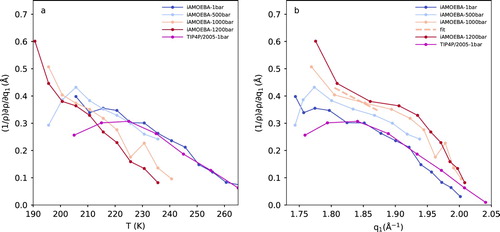
Figure 6 shows (1/ρ) × (∂ρ/∂q₁)_P for iAMOEBA and TIP4P/2005 simulations as a function of temperature as well as q₁. Figure 6(a) shows that there is a trend of continuous rise in (1/ρ) × (∂ρ/∂q₁)_P with decrease in temperature. There are no sharp changes in (1/ρ) × (∂ρ/∂q₁)_P corresponding to the maxima in (∂q₁/∂T)_P. This means that the temperature dependence of α is mostly determined by the temperature dependence of (∂q₁/∂T)_P, which is an important observation. One can also plot (1/ρ) × (∂ρ/∂q₁)_P with respect to q₁ as shown in Figure 6(b). Figure 6(b) shows that (1/ρ) × (∂ρ/∂q₁)_P increases with decrease in q₁ and for a given value of q₁, there is a general trend of higher (1/ρ) × (∂ρ/∂q₁)_P for higher pressures.

Figure 6. (1/ρ) × (∂ρ/∂q₁)_P, which is proportional to the thermal expansion coefficient as a function of (a) temperature and (b) first peak position (q₁) for simulations with a force–field of TIP4P/2005 at 1 bar and iAMOEBA at 1, 500, 1000 and 1200 bar. The q-range shown here covers the temperature range illustrated in Figure 6(a). Linear fit to the 1000 isobar is shown as a dashed line.

A linear fit to (1/ρ) × (∂ρ/∂q₁)_P for the 1000 bar isobar from Figure 6(b) is used together with Equation (2) in order to calculate α. We choose the 1 kbar isobar since it shows a close similarity to experimental (∂q₁/∂T)_P as shown in Figure 2. The resultant α is shown as ‘estimate1000bar’ in Figure 7. For comparison, α estimated from a linear fit from the isobar of 500 and 1200 bar from Figure 6(b) is also shown as ‘estimate500bar’ and ‘estimate1200bar’ respectively. In Figure 7, we illustrate that α shows a clear minimum for isobars of molecular dynamics simulations for the TIP4P/2005³⁸ and iAMOEBA force fields of water at ambient pressure. For iAMOEBA force field, the minimum shifts to lower temperatures as the pressure is increased and its location in terms of temperature coincides with the maxima observed in isothermal compressibility [23]. The estimates of α from 500, 1000 and 1200 bar are close to each other and we observe that α rapidly decreases with decrease in temperature until 229.2 K. Although this is an approximate way of determining α, the temperature dependence of α is accurately captured by these estimates. Figure 7 also illustrates the α determined by Hare and Sorenson [50] who fitted their density data to a 6th-degree polynomial equation down to 239.14 K. The temperature dependence of α is much steeper at colder temperatures and it is not accurately captured by ambient pressure isobars of iAMOEBA or TIP4P/2005 force-fields. However, the temperature dependence of α for 1 kbar iAMOEBA is close to our estimates. We see a rise in α for the two coldest temperatures where T < 229.2 K. However, we are aware that the possible error in our estimates of α is too high to definitely say if there exists a minimum at 229.2 K.

Figure 7. Thermal expansion coefficient (α) of water. Simulation data for iAMOEBA is shown for isobars of 1, 500, 1000 and 1200 bar respectively. TIP4P/2005 data are from ref. [38] (pink). The dashed line is the measurement from Hare and Sorenson [50]. ‘estimate500bar’, ‘estimate1000bar’ and ‘estimate1200bar’ are our estimations of α based on measured x-ray scattering spectra and estimated (1/ρ) × (∂ρ/∂q₁)_P from iAMOEBA curves in Figure 6(b).

Discussion

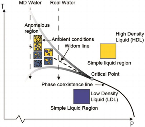
Figure 8 summarises the hypothesis that is consistent with all current experimental data [23]. There could exist two separate liquid phases, HDL and LDL, with a phase coexistence line in the P-T diagram deep in the supercooled regime and at elevated pressure [2,21]. This liquid–liquid transition (LLT) line terminates in the LLCP and its equivalent in the one-phase region corresponds to the Widom line [53]. At the Widom line, the density fluctuations would reach a maximum consistent with equal population of molecules in HDL and LDL [54]. Note that HDL is on the ambient temperature side of the Widom-line, whereas LDL is on the low temperature side. This explains why the high density, H-bond distorted species dominate at ambient conditions. The fluctuating anomalous region around the Widom line becomes wider on decreasing the pressure thereby, moving further away from the LLCP. The closer we are to the critical point, the narrower the region becomes and the stronger the anomalous behaviour will be, leading to steeper rise in the response functions. What is unique with water is that at ambient pressure, the location of the LLCP is such that the anomalous region with fluctuations extends up to around 320 K. At 320 K, water’s isothermal compressibility starts to increase with decreasing temperature.

Figure 8. Schematic picture of a hypothetical phase diagram of liquid water showing the liquid-liquid coexistence line between LDL and HDL in terms of simple liquid regions, the critical point (LLCP), the Widom line in the one-phase region and fluctuations on different length scales emanating from the critical point giving rise to local spatially separated regions in the anomalous region [11]. The shaded lines envelope the region where water behaves anomalously. The vertical dashed lines illustrate the cooling isobars of MD water (iAMOEBA and TIP4P/2005) and real water.

All experimental data presented here shows evidence of stronger anomalous fluctuations in comparison to the two force fields iAMOEBA and TIP4P/2005 used in the current study. Similar arguments have also been given regarding the E3B3 model [46]. What we note is that the deviation is not only for the coldest temperatures but all the way to ambient temperatures. The two vertical arrows in Figure 8 indicate the pressure relative to the LLCP of real water and simulated water. This means that real water is more anomalous than most MD water models because it is closer to the LLCP. Most likely this means that the fluctuating regions are less well defined in the simulations in comparison to real water [11]. There are further evidences for this in some recent X-ray spectroscopy investigations of ambient water with other comparisons between experiment and simulations [55] as well in recent intermediate scattering function measurements using speckle visibility spectroscopy [56]. It was observed that the timescale for the cage effects in real water becomes much shorter than what is seen in the TIP4P/2005 model, which is also reflected in the temperature dependence of the isothermal compressibility. Since the anomalous fluctuations are observed to be correlated with the growth of tetrahedral structures that form patches of around 1–2 nm size [11,20,23,39] depending on temperature, we assume that collective many body forces are essential to improve the simulation models [11].

In order to quantify the differences in anomalous fluctuations observed in simulations as compared to experiments, we have used the fact that the simulations show an enhancement in anomalous behaviour with increasing pressures towards the LLCP. The closer water is to a critical point, the stronger critical fluctuations are to be expected. Here we observe that the simulations qualitatively agree with the experimental data when shifted by ≈1 kbar. iAMOEBA and TIP4P/2005 have their critical point at 1750 [28] and 1700 bar [27] respectively. This means that for real water the LLCP, if it exists, would be located at ≈ 700 bar. This is consistent with recent estimates of LLCP, which were also derived by comparing experiments to simulations [23,46,49].

Conclusion

We have looked at experimental data of supercooled water and compared it to molecular simulations of two different force-fields of water, namely TIP4P/2005 and iAMOEBA. We have focused on the temperature dependent anomalous fluctuations related to the growth of tetrahedral structure, spatial correlation obtained from SAXS, thermodynamic response functions including isothermal compressibility and thermal expansion coefficients. Water’s thermal expansion coefficient has been estimated for the first time at deeply supercooled conditions from liquid water’s structure factor. Based on our observations, we conclude that ambient pressure water is best represented by molecular dynamics force-fields when simulated at ≈ 1 kbar pressure. This means that classical force field simulations underestimate the anomalous fluctuations in water extending from the Widom line to ambient temperatures.

Acknowledgements

We thank Dr. Lee-Ping Wang for providing thermodynamic properties of the iAMOEBA simulations in the deeply supercooled region.

Disclosure statement

No potential conflict of interest was reported by the authors.

Data availability statement

The authors confirm that the data supporting the findings of this study are available within the supplementary materials. Namely, the thermal expansion coefficient estimate for water depicted in Figure 7 is available.

ORCID

Harshad Pathak http://orcid.org/0000-0002-9284-4774

Additional information

Funding

This work was supported by H2020 European Research Council [grant number 667205]; Vetenskapsrådet [grant number 2013-8823].

References

- P. Gallo, K. Amann-Winkel, C.A. Angell, M.A. Anisimov, F.d.r. Caupin, C. Chakravarty, E. Lascaris, T. Loerting, A.Z. Panagiotopoulos and J. Russo, Chem. Rev. 116, 7463 (2016). doi: 10.1021/acs.chemrev.5b00750
- O. Mishima and H.E. Stanley, Nature. 396, 329 (1998). doi: 10.1038/24540
- H.E. Stanley, S.V. Buldyrev, O. Mishima, M.R. Sadr-Lahijany, A. Scala and F.W. Starr, J. Phys. Cond. Mat. 12, A403 (2000). doi: 10.1088/0953-8984/12/8A/355
- H.E. Stanley, S.V. Buldyrev, M. Canpolat, O. Mishima, M.R. Sadr-Lahijany, A. Scala and F.W. Starr, Phys. Chem. Chem. Phys. 2, 1551 (2000). doi: 10.1039/b000058m
- R.J. Speedy and C.A. Angell, J. Chem. Phys. 65, 851 (1976). doi: 10.1063/1.433153
- C.A. Angell, Ann. Rev. Phys. Chem. 34, 593 (1983). doi: 10.1146/annurev.pc.34.100183.003113
- P.G. Debenedetti, J. Phys. Cond. Matt. 15, R1669 (2003). doi: 10.1088/0953-8984/15/45/R01
- A. Nilsson and L.G.M. Pettersson, Chem. Phys. 389, 1 (2011). doi: 10.1016/j.chemphys.2011.07.021
- A. Angell, W.J. Sichina and M. Oguni, J. Phys. Chem. 86, 998 (1982). doi: 10.1021/j100395a032
- L.G.M. Pettersson and A. Nilsson, J. Non-Cryst. Solids. 407, 399 (2015). doi: 10.1016/j.jnoncrysol.2014.08.026
- A. Nilsson and L.G. Pettersson, Nat. Commun. 6, 8998 (2015). doi: 10.1038/ncomms9998
- J. Russo and H. Tanaka, Nat. Commun. 5, 3556 (2014). doi: 10.1038/ncomms4556
- P.G. Debenedetti, Metastable Liquids: Concepts and Principles (Princeton University Press, Princeton, New Jersey, USA, 1996).
- P. Ball, Chem. Rev. 108, 74 (2008). doi: 10.1021/cr068037a
- A. Nilsson, C. Huang and L.G.M. Pettersson, J. Mol. Liq. 176, 2 (2012). doi: 10.1016/j.molliq.2012.06.021
- L.G.M. Pettersson and A. Nilsson, J. Non-Cryst. Solids 407, 399–417 (2015). doi: 10.1016/j.jnoncrysol.2014.08.026
- A.K. Soper and M.A. Ricci, Phys. Rev. Lett. 84, 2881 (2000). doi: 10.1103/PhysRevLett.84.2881
- J. Russo, K. Akahane and H. Tanaka, Proc. Natl. Acad. Sci. U.S.A. 115, E3333 (2018). doi: 10.1073/pnas.1722339115
- V. Holten and M.A. Anisimov, Sci. Reps. 2, 713 (2012). doi: 10.1038/srep00713
- C. Huang, T.M. Weiss, D. Nordlund, K.T. Wikfeldt, L.G.M. Pettersson and A. Nilsson, J. Chem. Phys. 133, 134504 (2010). doi: 10.1063/1.3495974
- P.H. Poole, F. Sciortino, U. Essmann and H.E. Stanley, Nature. 360, 324 (1992). doi: 10.1038/360324a0
- P. Kumar, S.V. Buldyrev, S.V. Becker, P.H. Poole, F.W. Starr and H.E. Stanley, Proc. Natl. Acad. Sci. USA. 104, 9575 (2007). doi: 10.1073/pnas.0702608104
- K.H. Kim, A. Späh, H. Pathak, F. Perakis, D. Mariedahl, K. Amann-Winkel, J.A. Sellberg, J.H. Lee, S. Kim, J. Park, K.H. Nam, T. Katayama and A. Nilsson, Science. 358, 1589 (2017). doi: 10.1126/science.aap8269
- V. Holten, C. Qiu, E. Guillerm, M. Wilke, J. Rička, M. Frenz and F. Caupin, J. Phys. Chem. Lett. 8, 5519 (2017). doi: 10.1021/acs.jpclett.7b02563
- P. Gallo, D. Corradini and M. Rovere, Nat. Commun. 5, 5806 (2014). doi: 10.1038/ncomms6806
- J.L.F. Abascal and C. Vega, J. Chem. Phys. 133, 234502 (2010). doi: 10.1063/1.3506860
- R.S. Singh, J.W. Biddle, P.G. Debenedetti and M.A. Anisimov, J. Chem. Phys. 144, 144504 (2016). doi: 10.1063/1.4944986
- H. Pathak, J.C. Palmer, D. Schlesinger, K.T. Wikfeldt, J.A. Sellberg, L.G.M. Pettersson and A. Nilsson, J. Chem. Phys. 145, 134507 (2016). doi: 10.1063/1.4963913
- Y. Ni and J.L. Skinner, J. Chem. Phys. 144, 214501 (2016). doi: 10.1063/1.4952991
- Y. Li, J. Li and F. Wang, Proc. Natl. Acad. Sci. USA. 110, 12209 (2013). doi: 10.1073/pnas.1309042110
- J.C. Palmer, F. Martelli, Y. Liu, R. Car, A.Z. Panagiotopoulos and P.G. Debenedetti, Nature. 510, 385 (2014). doi: 10.1038/nature13405
- J.A. Sellberg, C. Huang, T.A. McQueen, N.D. Loh, H. Laksmono, D. Schlesinger, R.G. Sierra, D. Nordlund, C.Y. Hampton, D. Starodub, D.P. DePonte, M. Beye, C. Chen, A.V. Martin, A. Barty, K.T. Wikfeldt, T.M. Weiss, C. Caronna, J. Feldkamp, L.B. Skinner, M.M. Seibert, M. Messerschmidt, G.J. Williams, S. Boutet, L.G.M. Pettersson, M.J. Bogan and A. Nilsson, Nature. 510, 381 (2014). doi: 10.1038/nature13266
- L.B. Skinner, C. Huang, D. Schlesinger, L.G.M. Pettersson, A. Nilsson and C.J. Benmore, J. Chem. Phys. 138, 074506 (2013). doi: 10.1063/1.4790861
- T. Head-Gordon and G. Hura, Chem. Rev. 102, 2651 (2002). doi: 10.1021/cr0006831
- A.H. Narten and H.A. Levy, J. Chem. Phys. 55, 2263 (1971). doi: 10.1063/1.1676403
- L.B. Skinner, C.J. Benmore, J.C. Neuefeind and J.B. Parise, J. Chem. Phys. 141, 214507 (2014). doi: 10.1063/1.4902412
- H. Laksmono, T.A. McQueen, J.A. Sellberg, N.D. Loh, C. Huang, D. Schlesinger, R.G. Sierra, C.Y. Hampton, D. Nordlund, M. Beye, A.V. Martin, A. Barty, M.M. Seibert, M. Messerschmidt, G.J. Williams, S. Boutet, L.G.M. Pettersson, M.J. Bogan and A. Nilsson, J. Phys. Chem. Letters. 6, 2826–2832 (2015). doi: 10.1021/acs.jpclett.5b01164
- K.T. Wikfeldt, C. Huang, A. Nilsson and L.G.M. Pettersson, J. Chem. Phys. 134, 214506 (2011). doi: 10.1063/1.3594545
- C. Huang, K.T. Wikfeldt, T. Tokushima, D. Nordlund, Y. Harada, U. Bergmann, M. Niebuhr, T.M. Weiss, Y. Horikawa, M. Leetmaa, M.P. Ljungberg, O. Takahashi, A. Lenz, L. Ojamäe, A.P. Lyubartsev, S. Shin, L.G.M. Pettersson and A. Nilsson, Proc. Natl. Acad. Sci. U.S.A. 106, 15214 (2009). doi: 10.1073/pnas.0904743106
- F. Caupin, V. Holten, C. Qiu, E. Guillerm, M. Wilke, M. Frenz, J. Teixeira and A.K. Soper, Science. 360, eaat1634 (2018). doi: 10.1126/science.aat1634
- K.H. Kim, A. Späh, H. Pathak, F. Perakis, D. Mariedahl, K. Amann-Winkel, J.A. Sellberg, J.H. Lee, S. Kim, J. Park, K.H. Nam, T. Katayama and A. Nilsson, Science. 360, eaat1729 (2018). doi: 10.1126/science.aat1729
- L.-P. Wang, T. Head-Gordon, J.W. Ponder, P. Ren, J.D. Chodera, P.K. Eastman, T.J. Martinez and V.S. Pande, J. Phys. Chem. B. 117, 9956 (2013). doi: 10.1021/jp403802c
- J.W. Biddle, R.S. Singh, E.M. Sparano, F. Ricci, M.A. González, C. Valeriani, J.L.F. Abascal, P.G. Debenedetti, M.A. Anisimov and F. Caupin, J. Chem. Phys. 146, 034502 (2017). doi: 10.1063/1.4973546
- M.A. González, C. Valeriani, F. Caupin and J.L.F. Abascal, J. Chem. Phys. 145, 054505 (2016). doi: 10.1063/1.4960185
- V. Holten, J.C. Palmer, P.H. Poole, P.G. Debenedetti and M.A. Anisimov, J. Chem. Phys. 140, 104502 (2014). doi: 10.1063/1.4867287
- N.J. Hestand and J.L. Skinner, J. Chem. Phys. 149, 140901 (2018). doi: 10.1063/1.5046687
- Y.D. Fomin, V.N. Ryzhov, E.N. Tsiok and V.V. Brazhkin, Phys. Rev. E Stat. Nonlin. Soft Matter Phys. 91, 022111 (2015). doi: 10.1103/PhysRevE.91.022111
- P. Schienbein and D. Marx, Phys. Rev. E. 98, 022104 (2018). doi: 10.1103/PhysRevE.98.022104
- A. Späh, H. Pathak, K.H. Kim, F. Perakis, D. Mariedahl, K. Amann-Winkel, J.A. Sellberg, J.H. Lee, S. Kim, J. Park, K.H. Nam, T. Katayama and A. Nilsson, Phys. Chem. Chem. Phys. 21, 26 (2019). doi: 10.1039/C8CP05862H
- D.E. Hare and C.M. Sorensen, J. Chem. Phys. 87, 4840 (1987). doi: 10.1063/1.453710
- J. Wölk and R. Strey, J. Phys. Chem. B. 105, 11683 (2001).2O and D2O in Comparison: The Isotope Effect†. 11701 > doi: 10.1021/jp0115805
- G.S. Kell, J. Chem. Eng. Data. 20, 97 (1975). doi: 10.1021/je60064a005
- L. Xu, P. Kumar, S.V. Buldyrev, S.-H. Chen, P.H. Poole, F. Sciortino and H.E. Stanley, Proc. Natl. Acad. Sci. U.S.A. 102, 16558 (2005). doi: 10.1073/pnas.0507870102
- K.T. Wikfeldt, A. Nilsson and L.G.M. Pettersson, Phys. Chem. Chem. Phys. 13, 19918 (2011). doi: 10.1039/c1cp22076d
- I. Zhovtobriukh, N.A. Besley, T. Fransson, A. Nilsson and L.G.M. Pettersson, J. Chem. Phys. 148, 144507 (2018). doi: 10.1063/1.5009457
- F. Perakis, G. Camisasca, T.J. Lane, A. Späh, K.T. Wikfeldt, J.A. Sellberg, F. Lehmkühler, H. Pathak, K.H. Kim, K. Amann-Winkel, S. Schreck, S. Song, T. Sato, M. Sikorski, A. Eilert, T. McQueen, H. Ogasawara, D. Nordlund, W. Roseker, J. Koralek, S. Nelson, P. Hart, R. Alonso-Mori, Y. Feng, D. Zhu, A. Robert, G. Grübel, L.G.M. Pettersson and A. Nilsson, Nat. Commun. 9, 1917 (2018). doi: 10.1038/s41467-018-04330-5