Excited-state dynamics of molecules with classically driven trajectories and Gaussians

ABSTRACT

Simulating the dynamics of a molecule initiated in an excited electronic state constitutes a rather challenging task for theoretical and computational chemistry, as such dynamics leads to a strong coupling between nuclear motion and electronic states, that is, a breakdown of the Born–Oppenheimer approximation. This New Views article proposes a brief overview on recent theoretical developments aiming at simulating the excited-state dynamics of molecules – nonadiabatic molecular dynamics – focusing in particular on strategies employing travelling basis functions to portray the dynamics of nuclear wavefunctions. We start by discussing the central equations for nonadiabatic molecular dynamics in a Born–Huang representation. We then propose a comparison between two commonly employed strategies to simulate the excited-state dynamics of molecular systems in their full configuration space, Ab Initio Multiple Spawning (AIMS) and Trajectory Surface Hopping (TSH). The equations of motion for the two techniques are compared and used to contrast their respective description of phenomena involving the decoherence of nuclear wavepackets. Some recent works and developments of the AIMS method are then summarised. This New Views article ends with a highlight on the Exact Factorisation of the molecular wavefunction and how this approach contrasts with the more conventional Born–Huang picture when it comes to the description of photophysical and photochemical processes.

GRAPHICAL ABSTRACT

KEYWORDS:

• Excited-state dynamics
• nonadiabatic dynamics
• computational photochemistry
• surface hopping
• ab initio multiple spawning

1. Introduction

Many parts of our way to picture a molecule and its chemistry have been heavily influenced by the Born–Oppenheimer Approximation (BOA). Chemical structures, properties and reactivity are in many cases discussed mostly in terms of the evolution of nuclear degrees of freedom in a single electronic eigenstate – a direct result of the BOA, which completely decouples the motion of electrons and nuclei and thus introduces the concept of potential energy surfaces (PESs) [1,2]. As long as a molecule evolves in only one electronic eigenstate (usually the electronic ground state), the BOA provides a reliable framework for the theoretical treatment of its properties and reactivity. However, as soon as this molecule owns sufficient energy to encounter regions of the configuration space where nuclear motion can induce a change of electronic eigenstate, the BOA will break down. This occurs usually when the dynamics is initiated in an excited electronic state. During the relaxation process following this electronic excitation, the molecule will likely reach regions of nonadiabaticity, that is, regions where nuclear motion can potentially couple different electronic states, eventually leading to a change of electronic state. Consequently, a theoretical investigation of the time evolution of any photoexcited system is inherently connected with a molecular description that goes beyond the BOA – a challenge that has been actively tackled over the past decades [3].

The dynamics of a molecule in its excited electronic states is not just a curiosity for theoretical chemists, but is central for our understanding of photochemistry and its application in energy-related devices (light-emitting or photovoltaic materials), for example. A theoretical understanding of nonadiabatic processes is also central to support new experimental techniques, like ultrafast dynamics based on diffraction techniques (ultrafast electron and X-ray diffraction) that are directly sensitive to the spatial distribution of atoms. Through ultrafast electron diffraction, it was achieved to measure the nuclear motion in photoexcited molecular crystals with femtosecond resolution [4,5]. The time-resolved structural information obtained experimentally allows direct comparison with the results of simulations of nonadiabatic dynamics, as demonstrated in recent work [6–10]. Hence, these advances in experimental techniques also induced an increase in the importance of quantum dynamical simulations. The general interest for theoretical photochemistry is also reflected in the recent publication of several new textbooks on the topic – see , for example [11–14].

Different strategies have been proposed to describe the nuclear dynamics of an electronically excited molecule. The multiconfigurational time-dependent Hartree (MCTDH) [15–18] constitutes one of the most accurate methods available and alleviates the exponential cost of grid-based quantum dynamics strategies by using time-dependent single particle basis functions, propagated according to the Dirac–Frenkel principle. Although MCDTH still scales exponentially with the number of degrees of freedom, the base of the exponentiation is reduced to the number of single particle basis functions per degree of freedom (compared to the number of grid points in the standard method). Another strategy consists in expressing the nuclear wavefunctions using trajectory basis functions (TBFs). TBFs are 3$N_{\mathrm{N}}$-dimensional Gaussian functions (with $N_{\mathrm{N}}$ being the number of nuclei of the system) which can travel in position and momentum space, and form therefore a sort of moving grid of Gaussian functions. This idea is inspired by Heller's earlier work on expressing a nuclear wavepacket in terms of frozen Gaussians [19–22]. Following the idea of MCTDH, the equations of motion for the Gaussian functions can be determined through the Dirac–Frenkel variational principle, leading to the method called variational multiconfigurational Gaussian (vMCG) that offers a quantum propagation of the Gaussian parameters [23–25]. In multiconfigurational Ehrenfest (MCE), the Gaussian functions are propagated classically, following Ehrenfest trajectories [26–28]. As a result, the TBFs follow an average PES in regions of strong nonadiabaticity, composed of a linear combination of the adiabatic surfaces weighted by electronic coefficients. Alternatively, the method called full multiple spawning (FMS) proposes to evolve the Gaussian functions classically on adiabatic PESs [29–31]. The number of TBFs can, however, be expanded when nonadiabatic regions are encountered during the dynamics by using a spawning algorithm. More information on the FMS strategy will be provided in this New Views article.

While the methods mentioned above all formally incorporate the quantum nature of nuclei, the family of techniques coined mixed quantum/classical proposes to greatly simplify the dynamics by enforcing a classical approximation for the nuclei, while the electrons are still treated quantum-mechanically. In Ehrenfest dynamics, a mean-field potential energy is used to propagate the purely classical nuclei [32–34]. An extensively used mixed quantum/classical method is trajectory surface hopping (TSH), which represents the dynamics of a nuclear wavepacket by a swarm of independent classical trajectories that can hop between electronic states in regions of high nonadiabaticity [35,36]. The hopping probability is governed by electronic amplitudes integrated on the support of the classical trajectory, with the most commonly used hopping criterion being the fewest switches algorithm [37–39]. More information on TSH will be given below.

Note that apart from these strategies, a variety of other formalisms has been developed to describe non-Born–Oppenheimer dynamics, such as semiclassical approaches [40–42], including e.g. mapping approaches [43–47], quantum-classical Liouville methods [48–50], Bohmian dynamics [51–54] or quantum trajectory mean-field dynamics [55].

In this New Views article, we propose an introduction to the central equations of nonadiabatic molecular dynamics, highlighting the key required quantities for their solution – electronic structure and nuclear dynamics. We focus on the FMS framework and its current developments, also highlighting how its formalism compares to the commonly employed TSH strategy. We finally discuss new perspectives on excited-state dynamics offered by the so-called Exact Factorisation of the molecular wavefunction.

2. Born–Huang approach to nonadiabatic dynamics

In the following, we will introduce the central equations for nonadiabatic quantum dynamics within the so-called Born–Huang representation of the molecular wavefunction. These equations constitute the cornerstone for the FMS method that will be described later in this New Views article. Solving the nonadiabatic quantum dynamics equations requires specific information about the electronic structure of the molecule, and we briefly discuss some of the main techniques employed for this purpose and the limitations of their approximations. Last but not least, we highlight the link between the Born–Huang representation and concepts of photochemistry.

2.1. Time-dependent molecular wavefunction

Any urge towards a quantum-mechanical description of a (pure state) system is indispensably connected to a treatment of its wavefunction. The wavefunction is an element of the Hilbert space of square-integrable functions and contains the information on all properties of the system. If the system under consideration is a molecule, one needs to consider its molecular wavefunction $\mathrm{\Psi }(\mathit{r},\mathit{R},t)$, which depends on the 3$N_{\mathrm{e}\mathrm{l}}$ electronic and 3$N_{\mathrm{N}}$ nuclear coordinates, collected in $\mathit{r}$ and $\mathit{R}$, respectively, and the time t. Characterising the time dependence of the molecular wavefunction, sometimes referred to as its ‘quantum molecular dynamics’, implies the solution of the time-dependent molecular Schrödinger equation. Within a nonrelativistic framework, the time-dependent Schrödinger equation for a molecule, in atomic units, reads (1) $i\frac{\mathrm{\partial }}{\mathrm{\partial }t}\mathrm{\Psi }(\mathit{r},\mathit{R},t)=\hat{H}(\mathit{r},\mathit{R})\mathrm{\Psi }(\mathit{r},\mathit{R},t).$(1) The molecular Hamiltonian $\hat{H}(\mathit{r},\mathit{R})$ can be separated into a sum of a nuclear kinetic energy operator ${\hat{T}}_{\mathrm{N}}\left(\mathit{R}\right)$ and an electronic Hamiltonian ${\hat{\mathcal{H}}}_{\mathrm{e}\mathrm{l}}(\mathit{r},\mathit{R})$, taking the form (2) $\begin{array}{rl}\hat{H}(\mathit{r},\mathit{R})& =-\sum _{\gamma }^{N_{\mathrm{N}}}\frac{1}{2M_{\gamma }}{\mathrm{\nabla }}_{\gamma }^2-\sum _i^{N_{\mathrm{e}\mathrm{l}}}\frac{1}{2}{\mathrm{\nabla }}_i^2+\sum _{i<j}\frac{1}{|{\mathit{r}}_i-{\mathit{r}}_j|}\\ & -\sum _{\gamma ,i}\frac{Z_{\gamma }}{|{\mathit{R}}_{\gamma }-{\mathit{r}}_i|}+\sum _{\gamma <\text{β}}\frac{Z_{\gamma }{Z}_{\text{β}}}{|{\mathit{R}}_{\gamma }-{\mathit{R}}_{\text{β}}|}\\ & =-\sum _{\gamma }^{N_{\mathrm{N}}}\frac{1}{2M_{\gamma }}{\mathrm{\nabla }}_{\gamma }^2+{\hat{\mathcal{H}}}_{\mathrm{e}\mathrm{l}}(\mathit{r},\mathit{R})\\ & ={\hat{T}}_{\mathrm{N}}\left(\mathit{R}\right)+{\hat{\mathcal{H}}}_{\mathrm{e}\mathrm{l}}(\mathit{r},\mathit{R}).\end{array}$(2) ${\hat{\mathcal{H}}}_{\mathrm{e}\mathrm{l}}$ includes the kinetic energy operator for the electrons as well as all the operators for Coulombic interactions related to the electrons and nuclei. For a given nuclear configuration $\mathit{R}$, the time-independent electronic Schrödinger equation provides an eigenvalue equation for the ${\hat{\mathcal{H}}}_{\mathrm{e}\mathrm{l}}$ Hamiltonian, (3) ${\hat{\mathcal{H}}}_{\mathrm{e}\mathrm{l}}(\mathit{r},\mathit{R}){\mathrm{\Phi }}_J(\mathit{r};\mathit{R})=E_J^{\mathrm{e}\mathrm{l}}\left(\mathit{R}\right){\mathrm{\Phi }}_J(\mathit{r};\mathit{R}),$(3) producing a set of orthonormal electronic basis functions, $\left\{{\mathrm{\Phi }}_J\right(\mathit{r};\mathit{R}\left)\right\}$, called electronic (adiabatic) wavefunctions with J being a label denoting the electronic state, and associated with the electronic energies $E_J^{\mathrm{e}\mathrm{l}}\left(\mathit{R}\right)$. Using this orthonormal basis to expand our molecular wavefunction leads to the so-called Born–Huang (BH) representation [56] (4) $\mathrm{\Psi }(\mathit{r},\mathit{R},t)=\sum _J^{\mathrm{\infty }}{\mathrm{\Phi }}_J(\mathit{r};\mathit{R}){\chi }_J(\mathit{R},t).$(4) (Note that the sum can run over explicit quantum numbers or over states.) It is important to realise that the BH representation groups all the time dependence of the molecular wavefunction in the expansion coefficients ${\chi }_J(\mathit{R},t)$, which correspond to time-dependent nuclear wavefunctions for each electronic state J.

By inserting the BH representation (Equation 4(4) $\mathrm{\Psi }(\mathit{r},\mathit{R},t)=\sum _J^{\mathrm{\infty }}{\mathrm{\Phi }}_J(\mathit{r};\mathit{R}){\chi }_J(\mathit{R},t).$(4) ) into the time-dependent Schrödinger equation (Equation 1(1) $i\frac{\mathrm{\partial }}{\mathrm{\partial }t}\mathrm{\Psi }(\mathit{r},\mathit{R},t)=\hat{H}(\mathit{r},\mathit{R})\mathrm{\Psi }(\mathit{r},\mathit{R},t).$(1) ), one obtains a series of coupled equations of motion for the nuclear amplitudes (upon left multiplication by ${\mathrm{\Phi }}_I^{\ast }(\mathit{r};\mathit{R})$ and integration over all electronic coordinates $\mathit{r}$), (5) $\begin{array}{rl}i\frac{\mathrm{\partial }{\chi }_I(\mathit{R},t)}{\mathrm{\partial }t}& =\left[{\hat{T}}_{\mathrm{N}}\left(\mathit{R}\right)+E_I^{\mathrm{e}\mathrm{l}}\left(\mathit{R}\right)\right]{\chi }_I(\mathit{R},t)\\ & -\sum _J^{\mathrm{\infty }}\left[\sum _{\rho }^{3N_{\mathrm{N}}}\left[\phantom{\sum _{\rho }^{3N_{\mathrm{N}}}}\frac{1}{M_{\rho }}⟨{\mathrm{\Phi }}_I|\frac{\mathrm{\partial }}{\mathrm{\partial }{R}_{\rho }}|{\mathrm{\Phi }}_J{⟩}_{\mathit{r}}\frac{\mathrm{\partial }}{\mathrm{\partial }{R}_{\rho }}\right.\right.\\ & +\left.\left.\frac{1}{2M_{\rho }}⟨{\mathrm{\Phi }}_I|\frac{{\mathrm{\partial }}^2}{\mathrm{\partial }{R}_{\rho }^2}|{\mathrm{\Phi }}_J{⟩}_{\mathit{r}}\right]\right]{\chi }_J(\mathit{R},t).\end{array}$(5) The first square-bracket term on the right-hand side of Equation (5(5) $\begin{array}{rl}i\frac{\mathrm{\partial }{\chi }_I(\mathit{R},t)}{\mathrm{\partial }t}& =\left[{\hat{T}}_{\mathrm{N}}\left(\mathit{R}\right)+E_I^{\mathrm{e}\mathrm{l}}\left(\mathit{R}\right)\right]{\chi }_I(\mathit{R},t)\\ & -\sum _J^{\mathrm{\infty }}\left[\sum _{\rho }^{3N_{\mathrm{N}}}\left[\phantom{\sum _{\rho }^{3N_{\mathrm{N}}}}\frac{1}{M_{\rho }}⟨{\mathrm{\Phi }}_I|\frac{\mathrm{\partial }}{\mathrm{\partial }{R}_{\rho }}|{\mathrm{\Phi }}_J{⟩}_{\mathit{r}}\frac{\mathrm{\partial }}{\mathrm{\partial }{R}_{\rho }}\right.\right.\\ & +\left.\left.\frac{1}{2M_{\rho }}⟨{\mathrm{\Phi }}_I|\frac{{\mathrm{\partial }}^2}{\mathrm{\partial }{R}_{\rho }^2}|{\mathrm{\Phi }}_J{⟩}_{\mathit{r}}\right]\right]{\chi }_J(\mathit{R},t).\end{array}$(5) ) describes the evolution of the nuclear wavefunction ${\chi }_I(\mathit{R},t)$ on the Ith electronic state, with the corresponding PES arising from $E_I^{\mathrm{e}\mathrm{l}}\left(\mathit{R}\right)$. The second square-bracket term introduces couplings between nuclear amplitudes evolving on different electronic states through the first- and second-order nonadiabatic derivative couplings, ${\mathit{d}}_{IJ}\left(\mathit{R}\right)=⟨{\mathrm{\Phi }}_I|{\mathrm{\nabla }}_{\mathit{R}}|{\mathrm{\Phi }}_J{⟩}_{\mathit{r}}$ and $D_{IJ}\left(\mathit{R}\right)=⟨{\mathrm{\Phi }}_I|{\mathrm{\nabla }}_{\mathit{R}}^2|{\mathrm{\Phi }}_J{⟩}_{\mathit{r}}$, respectively. The notation $⟨\cdots {⟩}_{\mathit{r}}$ means integration over $\mathit{r}$. (We note that $D_{II}\left(\mathit{R}\right)$ is non-zero and also contributes an additional term within a given electronic state I.)

2.2. Electronic structure for nonadiabatic dynamics

The previously derived set of equations of motion for nuclear amplitudes, Equation (5(5) $\begin{array}{rl}i\frac{\mathrm{\partial }{\chi }_I(\mathit{R},t)}{\mathrm{\partial }t}& =\left[{\hat{T}}_{\mathrm{N}}\left(\mathit{R}\right)+E_I^{\mathrm{e}\mathrm{l}}\left(\mathit{R}\right)\right]{\chi }_I(\mathit{R},t)\\ & -\sum _J^{\mathrm{\infty }}\left[\sum _{\rho }^{3N_{\mathrm{N}}}\left[\phantom{\sum _{\rho }^{3N_{\mathrm{N}}}}\frac{1}{M_{\rho }}⟨{\mathrm{\Phi }}_I|\frac{\mathrm{\partial }}{\mathrm{\partial }{R}_{\rho }}|{\mathrm{\Phi }}_J{⟩}_{\mathit{r}}\frac{\mathrm{\partial }}{\mathrm{\partial }{R}_{\rho }}\right.\right.\\ & +\left.\left.\frac{1}{2M_{\rho }}⟨{\mathrm{\Phi }}_I|\frac{{\mathrm{\partial }}^2}{\mathrm{\partial }{R}_{\rho }^2}|{\mathrm{\Phi }}_J{⟩}_{\mathit{r}}\right]\right]{\chi }_J(\mathit{R},t).\end{array}$(5) ), makes it clear that a solution of the time-dependent Schrödinger equation in the adiabatic representation requires knowledge of the following electronic information: electronic energies $E_I^{\mathrm{e}\mathrm{l}}\left(\mathit{R}\right)$, nonadiabatic coupling vectors ${\mathit{d}}_{IJ}\left(\mathit{R}\right)$, and potentially the gradients of the electronic energies and second-order nonadiabatic couplings $D_{IJ}\left(\mathit{R}\right)$, for and between all electronic states considered. These quantities can be obtained from a vast range of methods that aim at approximating the time-independent electronic Schrödinger equation  (3(3) ${\hat{\mathcal{H}}}_{\mathrm{e}\mathrm{l}}(\mathit{r},\mathit{R}){\mathrm{\Phi }}_J(\mathit{r};\mathit{R})=E_J^{\mathrm{e}\mathrm{l}}\left(\mathit{R}\right){\mathrm{\Phi }}_J(\mathit{r};\mathit{R}),$(3) ), with critical caveats and limitations existing for any of these electronic structure methods. It goes beyond the scope of this New Views article to detail all electronic structure techniques that can be used for excited electronic states, and we invite the interested reader to consult some of the numerous reviews or book chapters available on this subject [57–67]. We only provide here a brief list of the most commonly employed electronic structure methods: (SA-)CASSCF [68,69] (state-averaged complete active space self-consistent field), MRCI [70] (multireference configuration interaction), MS-CASPT2 [71] (multistate complete active space perturbation of second order), ADC(2) [72,73] (algebraic diagrammatic construction of second order), LR-TDDFT [74–76] (linear-response time-dependent density functional theory), FOMO-CASCI [77,78] (floating occupation molecular orbital complete active space configuration interaction) or MRCI-OM2 [79] (MRCI based on the orthogonalisation method 2).

Ideally, an electronic structure method would (i) provide all the quantities we need for the nuclear dynamics, (ii) describe equally well the different electronic states of interest, (iii) be able to describe accurately the couplings between electronic states, (iv) be efficient if used in combination with on-the-fly (direct) dynamics (see below), (v) be robust enough when visiting different regions of the configuration space, (vi) capable of describing (or at least detecting) multiconfigurational character of the electronic wavefunction(s). Unfortunately, none of the methods listed above offers an optimal compromise for nonadiabatic molecular dynamics and we highlight here some of the most serious issues for different methods.

While being one of the most commonly employed methods for trajectory-based nonadiabatic dynamics, (SA-)CASSCF suffers from its neglect of dynamic correlation, leading to a potentially imbalanced description of electronic states [59].

LR-TDDFT, within the adiabatic approximation for the exchange-correlation kernel [61], can fail to describe electronic states with a charge-transfer character [80–86], conical intersections between the ground and first excited state [87], electronic states with double-excitation character [87–91], and can formally only be used to describe ground-to-excited-state quantities like nonadiabatic coupling vectors [92–99] (or spin–orbit coupling matrix elements [100]), even if linear-response theory already offers a good approximation [101] (quadratic response theory can be used but unstable within the adiabatic approximation [99,102,103]). Different benchmarks of LR-TDDFT and exchange/correlation functionals for the description of electronic energies have been proposed in the literature (see , e.g. [104] for a review of benchmarks), and we highlight here only more specific benchmarks related to oscillator strengths [105], singlet/triplet splitting [106], spin–orbit couplings [107] and nonadiabatic dynamics [108].

ADC(2), in its standard formulation, cannot be used to describe the coupling between the ground and first excited state but a spin-flip variant has recently been proposed [109]. CC2 (second-order approximate coupled cluster) suffers from instabilities in regions where electronic states are degenerate [103,108] and work to solve this issue recently appeared in the literature [110,111].

Besides its computational cost, (MS-)CASPT2 may suffer from the appearance of intruder states and instabilities near conical intersection [59,112].

Nonadiabatic dynamics techniques can be classified into two families based on when the electronic structure quantities are calculated. Some nuclear dynamics strategies require a global knowledge of the PESs and couplings over the entire nuclear configuration space considered. Therefore, such methods necessitate the precalculation of all electronic structure quantities prior to the actual nuclear propagation. They also often rely on the fitting of the electronic structure quantities to certain functional forms or on the use of a model Hamiltonian [113,114]. Contrarily, other nonadiabatic methods only require the electronic structure information to be known locally, allowing for on-the-fly nonadiabatic dynamics (also called ‘direct’ or ‘ab initio’ dynamics). In this case, the electronic quantities are computed at each nuclear propagation time step or when required.¹ The cost of electronic structure calculations can become a serious bottleneck when performing on-the-fly excited-state dynamics of molecular systems. Recent developments could achieve a dramatic reduction of this computational cost, for instance by combining nonadiabatic dynamics with quantum chemical calculations accelerated on graphics processing units (GPUs) (see for example Refs. [117–120]) or by employing machine (or deep-) learning strategies [121,122,123].

Finally, it is crucial to highlight the importance of carefully testing the different quantum-chemical methods available to describe the electronic structure of a molecule, prior to any excited-state dynamics and beyond the Franck–Condon region. Critical points of the PES(s) – minima, minimum-energy conical intersections, minimum energy crossing points, branching space of important conical intersections – should be first located at the highest level of theory possible. Pathways produced by linear interpolations in internal coordinates (LIICs) can be employed to connect critical points (see , e.g. [124] and its supporting information) and to ensure the electronic structure method of interest for the dynamics reproduces the trends of higher level methods. The first trajectories then calculated with the chosen best compromise for the electronic structure – efficiency vs accuracy – can be used to once more check the adequacy of the electronic structure technique. A similar protocol can be employed for other electronic structure quantities that may be required, for example when trying to reproduce theoretically experimental observables for comparison.

2.3. Side note – Born–Huang representation and photochemistry

Our understanding of photochemical and photophysical processes is rooted in the previously introduced Born–Huang representation: one often thinks about excited-state molecular processes in terms of a molecule transferring between different electronic states during nonradiative relaxation processes – exactly what the set of coupled equations (5(5) $\begin{array}{rl}i\frac{\mathrm{\partial }{\chi }_I(\mathit{R},t)}{\mathrm{\partial }t}& =\left[{\hat{T}}_{\mathrm{N}}\left(\mathit{R}\right)+E_I^{\mathrm{e}\mathrm{l}}\left(\mathit{R}\right)\right]{\chi }_I(\mathit{R},t)\\ & -\sum _J^{\mathrm{\infty }}\left[\sum _{\rho }^{3N_{\mathrm{N}}}\left[\phantom{\sum _{\rho }^{3N_{\mathrm{N}}}}\frac{1}{M_{\rho }}⟨{\mathrm{\Phi }}_I|\frac{\mathrm{\partial }}{\mathrm{\partial }{R}_{\rho }}|{\mathrm{\Phi }}_J{⟩}_{\mathit{r}}\frac{\mathrm{\partial }}{\mathrm{\partial }{R}_{\rho }}\right.\right.\\ & +\left.\left.\frac{1}{2M_{\rho }}⟨{\mathrm{\Phi }}_I|\frac{{\mathrm{\partial }}^2}{\mathrm{\partial }{R}_{\rho }^2}|{\mathrm{\Phi }}_J{⟩}_{\mathit{r}}\right]\right]{\chi }_J(\mathit{R},t).\end{array}$(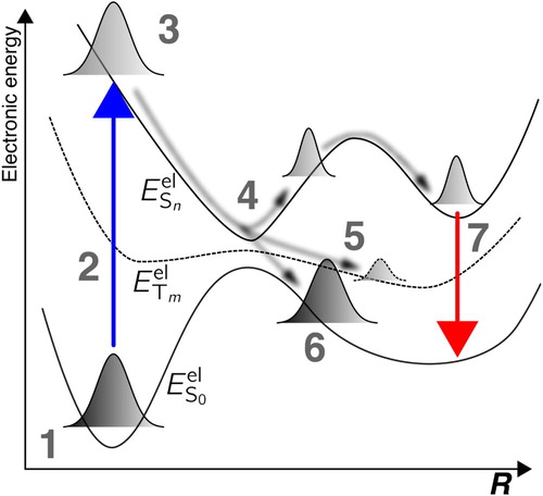5) ) describes. A typical Born–Huang picture of photochemistry is represented schematically in Figure 1. A molecule is originally in its ground electronic and vibrational state (1) when an ultrashort pulse of light triggers an electronic excitation (2) towards a certain excited electronic state S${}_n$, based on the interaction between the light pulse and the molecule. If the pulse is short enough, the original nuclear wavefunction in S${}_0$ is projected onto the excited electronic state to form a nuclear wavepacket (3) – the original nuclear wavefunction is represented in excited state S${}_n$ as a linear combination of the nuclear eigenstates of this new electronic state. The nuclear wavepacket in electronic state S${}_n$, ${\chi }_{{\mathrm{S}}_n}(\mathit{R},t)$, relaxes (4) and is likely to reach regions of strong nonadiabaticity, i.e. regions where electronic states are close in energy and can be coupled by nuclear motion, as described above. In such regions, the nuclear wavepacket will transfer amplitude towards the coupled electronic states, leading to a splitting or a branching on a different electronic state with same (6) or different (5) spin multiplicity. Such a relaxation process is called nonradiative decay, and more precisely internal conversion if the electronic states considered all share the same spin multiplicity or intersystem crossings whenever they have different spin multiplicities. If the nuclear wavepacket is trapped in a region (minimum) of an excited state² for a time long enough, luminescence can be observed: the molecule relaxes to the ground state via light emission (7). Let us note at this stage that solving the Schrödinger equation with the Hamiltonian introduced in Equation (2(2) $\begin{array}{rl}\hat{H}(\mathit{r},\mathit{R})& =-\sum _{\gamma }^{N_{\mathrm{N}}}\frac{1}{2M_{\gamma }}{\mathrm{\nabla }}_{\gamma }^2-\sum _i^{N_{\mathrm{e}\mathrm{l}}}\frac{1}{2}{\mathrm{\nabla }}_i^2+\sum _{i<j}\frac{1}{|{\mathit{r}}_i-{\mathit{r}}_j|}\\ & -\sum _{\gamma ,i}\frac{Z_{\gamma }}{|{\mathit{R}}_{\gamma }-{\mathit{r}}_i|}+\sum _{\gamma <\text{β}}\frac{Z_{\gamma }{Z}_{\text{β}}}{|{\mathit{R}}_{\gamma }-{\mathit{R}}_{\text{β}}|}\\ & =-\sum _{\gamma }^{N_{\mathrm{N}}}\frac{1}{2M_{\gamma }}{\mathrm{\nabla }}_{\gamma }^2+{\hat{\mathcal{H}}}_{\mathrm{e}\mathrm{l}}(\mathit{r},\mathit{R})\\ & ={\hat{T}}_{\mathrm{N}}\left(\mathit{R}\right)+{\hat{\mathcal{H}}}_{\mathrm{e}\mathrm{l}}(\mathit{r},\mathit{R}).\end{array}$(2) ) does not allow to observe the processes of light absorption (2), light emission (7) or intersystem crossings (6) – see Section 3.2.4 for more details. The discussion of photochemical processes in terms of static and coupled PESs on which nuclear wavepackets evolve is a direct by-product of the Born–Huang representation of the molecular wavefunction.

Figure 1. Schematic representation of a molecular photoexcitation and the subsequent photochemical and photophysical processes. The different steps are discussed in the main text.

3. Nonadiabatic molecular dynamics

Now that the main equations and ingredients for nonadiabatic dynamics have been defined, let us discuss how such a dynamics can be performed in practice for molecular systems. We start from the full description of nuclear quantum effects, moving then to an expansion of the nuclear amplitudes in a basis of TBFs, and finishing with a more approximate description of nuclear probability densities as a swarm of classical independent trajectories.

3.1. Expressing the nuclear amplitudes in a basis of time-dependent functions

Let us start by considering the nuclear wavefunction in electronic state J, ${\chi }_J(\mathit{R},t)$, and expand it in a basis of $N_{\mathrm{B}\mathrm{F}\mathrm{s}}^J$ basis functions, $\{{\tilde{\chi }}_k^J{\}}_{k=1}^{N_{\mathrm{B}\mathrm{F}\mathrm{s}}^J}$, with ${\tilde{\chi }}_k^{\left(J\right)}:={\tilde{\chi }}_k^{\left(J\right)}(\mathit{R};a_{k,1}^{\left(J\right)}(t),\dots ,a_{k,N_{\mathrm{P}}}^{\left(J\right)}(t\left)\right)$ (with $\left\{a_{k,i}^{\left(J\right)}\right(t){\}}_{i=1}^{N_{\mathrm{P}}}$ being a set of $N_{\mathrm{P}}$ time-dependent parameters). Inserting this basis expansion into the BH representation results in the following form of the molecular wavefunction: (6) $\begin{array}{rl}\mathrm{\Psi }(\mathit{r},\mathit{R},t)& =\sum _J^{\mathrm{\infty }}\sum _k^{N_{\mathrm{B}\mathrm{F}\mathrm{s}}^J}{C}_k^{\left(J\right)}\left(t\right){\tilde{\chi }}_k^{\left(J\right)}(\mathit{R};a_{k,1}^{\left(J\right)}(t),\dots ,a_{k,N_{\mathrm{P}}}^{\left(J\right)}(t\left)\right){\mathrm{\Phi }}_J(\mathit{r};\mathit{R}),\end{array}$(6) with $\{C_k^{\left(J\right)}{\}}_{k=1}^{N_{\mathrm{B}\mathrm{F}\mathrm{s}}^J}$ being complex time-dependent expansion coefficients associated with the electronic state J. If one inserts this form of the BH representation into the TDSE (Equation 1(1) $i\frac{\mathrm{\partial }}{\mathrm{\partial }t}\mathrm{\Psi }(\mathit{r},\mathit{R},t)=\hat{H}(\mathit{r},\mathit{R})\mathrm{\Psi }(\mathit{r},\mathit{R},t).$(1) ), left-multiplies the result by $\left({\tilde{\chi }}_{k^{\prime }}^{\left(I\right)}\right(\mathit{R};a_{k^{\prime },1}^{\left(I\right)}\left(t\right),\dots ,a_{k^{\prime },N_{\mathrm{P}}}^{\left(I\right)}\left(t\right)\left){\mathrm{\Phi }}_I\right(\mathit{r};\mathit{R}){)}^{\ast }$ and integrates over all electronic ($\mathit{r}$) as well as nuclear coordinates ($\mathit{R}$), a set of equations of motion for the complex expansion coefficients can be deduced and reads, in matrix form, (7) $\dot{\mathit{C}}=-i{\mathit{S}}^{-1}\left[\right(\mathit{H}-i\dot{\mathit{S}}\left)\mathit{C}\right].$(7) This is nothing but the time-dependent molecular Schrödinger equation expressed within a basis of electronic eigenfunctions ($\left\{{\mathrm{\Phi }}_J\right(\mathit{r};\mathit{R}\left)\right\}$) and a basis of nonorthogonal functions ($\{{\tilde{\chi }}_k^J{\}}_{k=1}^{N_{\mathrm{B}\mathrm{F}\mathrm{s}}^J}$). One finds in Equation (7(7) $\dot{\mathit{C}}=-i{\mathit{S}}^{-1}\left[\right(\mathit{H}-i\dot{\mathit{S}}\left)\mathit{C}\right].$(7) ) the overlap matrix $(\mathit{S}{)}_{k{k}^{\prime }}^{IJ}=⟨{\tilde{\chi }}_k^{\left(I\right)}|{\tilde{\chi }}_{k^{\prime }}^{\left(J\right)}{⟩}_{\mathit{R}}{\delta }_{IJ}$, the Hamiltonian matrix $(\mathit{H}{)}_{k{k}^{\prime }}^{IJ}=⟨{\mathrm{\Phi }}_I{\tilde{\chi }}_k^{\left(I\right)}|\hat{H}|{\tilde{\chi }}_{k^{\prime }}^{\left(J\right)}{\mathrm{\Phi }}_J{⟩}_{\mathit{r},\mathit{R}}$ and an overlap matrix including the time derivatives of the basis functions $(\dot{\mathit{S}}{)}_{k{k}^{\prime }}^{IJ}=⟨{\tilde{\chi }}_k^{\left(I\right)}|(\mathrm{\partial }/\mathrm{\partial }t){\tilde{\chi }}_{k^{\prime }}^{\left(J\right)}{⟩}_{\mathit{R}}{\delta }_{IJ}$. Importantly, the form of Equation (7(7) $\dot{\mathit{C}}=-i{\mathit{S}}^{-1}\left[\right(\mathit{H}-i\dot{\mathit{S}}\left)\mathit{C}\right].$(7) ) indicates that all the basis functions are coupled in an intra- as well as an interstate manner.

The definition of the basis functions $\{{\tilde{\chi }}_k^{\left(J\right)}{\}}_{k=1}^{N_{\mathrm{B}\mathrm{F}\mathrm{s}}^J}$, the approach to describe the evolution of its time-dependent parameters as well as the way to compute or approximate the matrix elements of Equation (7(7) $\dot{\mathit{C}}=-i{\mathit{S}}^{-1}\left[\right(\mathit{H}-i\dot{\mathit{S}}\left)\mathit{C}\right].$(7) ) are what differentiates the various methods for nonadiabatic quantum molecular dynamics. The variational Multiconfigurational Gaussian (vMCG) method proposes to employ the Dirac–Frenkel variational principle to propagate the basis functions, taken as multidimensional Gaussians, and their parameters [23–25,125–127]. In multiconfigurational Ehrenfest (MCE), the (frozen) Gaussians follow Ehrenfest trajectories [26–28,128]. Other alternative formulations of the total molecular wavefunction using TBFs were proposed more recently [129,130]. In the following, we will focus on the Full (FMS) and Ab Initio Multiple Spawning (AIMS) methods that utilise a basis of frozen multidimensional Gaussian functions which evolve according to classical laws of motion.

3.2. Full- and ab initio multiple spawning

3.2.1. Equations of motion

FMS [29,31,131–136] is based on the idea of expanding the nuclear wavefunctions into a basis of moving multidimensional Gaussian functions (the basis functions described earlier and now called trajectory basis functions – TBFs), (8) $\begin{array}{rl}{\chi }_J(\mathit{R},t)& :=\sum _k^{N_{\mathrm{T}\mathrm{B}\mathrm{F}\mathrm{s}}^J}{C}_k^{\left(J\right)}\left(t\right){\tilde{\chi }}_k^{\left(J\right)}\left(\mathit{R};{\overline{\mathit{R}}}_k^{\left(J\right)}\left(t\right),{\overline{\mathit{P}}}_k^{\left(J\right)}\left(t\right),{\overline{\gamma }}_k^{\left(J\right)}\left(t\right),\mathit{\alpha }\right).\end{array}$(8) The time dependence of the basis set is apparent in the definition of the position, ${\overline{\mathit{R}}}_k^{\left(J\right)}\left(t\right)$, and momentum, ${\overline{\mathit{P}}}_k^{\left(J\right)}\left(t\right)$, of the centre of the TBF, as well as a phase, ${\overline{\gamma }}_k^{\left(J\right)}\left(t\right)$. Since FMS utilises an ansatz of frozen Gaussians, their width, $\mathit{\alpha }$, will be time independent. Each $3N_{\mathrm{N}}$-dimensional TBF is constructed as a product of 3$N_{\mathrm{N}}$ one-dimensional Gaussian functions, i.e. (9) $\begin{array}{rl}& {\tilde{\chi }}_k^{\left(J\right)}\left(\mathit{R};{\overline{\mathit{R}}}_k^{\left(J\right)}\left(t\right),{\overline{\mathit{P}}}_k^{\left(J\right)}\left(t\right),{\overline{\gamma }}_k^{\left(J\right)}\left(t\right),\mathit{\alpha }\right)\\ & =e^{i{\overline{\gamma }}_k^{\left(J\right)}\left(t\right)}\prod _{\rho }^{3N_{\mathrm{N}}}{\tilde{\chi }}_{k\rho }^{\left(J\right)}(R_{\rho };{\overline{R}}_{k\rho }^{\left(J\right)}(t),{\overline{P}}_{k\rho }^{\left(J\right)}(t),{\alpha }_{\rho })\end{array}$(9) (10) $\begin{array}{rl}& {\tilde{\chi }}_{k\rho }^{\left(J\right)}(R_{\rho };{\overline{R}}_{k\rho }^{\left(J\right)}(t),{\overline{P}}_{k\rho }^{\left(J\right)}(t),{\alpha }_{\rho })\\ & ={\left(\frac{2{\alpha }_{\rho }}{\pi }\right)}^{1/4}\exp \left[-{\alpha }_{\rho }{\left(R_{\rho }-{\overline{R}}_{k\rho }^{\left(J\right)}\left(t\right)\right)}^2\right.\\ & +\left.i{\overline{P}}_{k\rho }^{\left(J\right)}\left(t\right)\left(R_{\rho }-{\overline{R}}_{k\rho }^{\left(J\right)}\left(t\right)\right)\phantom{\sum }\right],\end{array}$(10) and their centre in position and momentum space will evolve based on Hamilton's equations of motion [134,136].

In FMS, the initial molecular wavefunction of the system is expressed as a linear combination of $N_{\mathrm{i}\mathrm{n}\mathrm{i}}$ coupled parent wavefunctions. For each of these parent molecular wavefunctions, one can write an FMS version of the BH representation, leading to the following representation of the molecular wavefunction: (11) $\begin{array}{rl}\mathrm{\Psi }(\mathit{r},\mathit{R},t)& =\sum _{\text{β}}^{N_{\mathrm{i}\mathrm{n}\mathrm{i}}}{\tilde{\mathrm{\Psi }}}_{\text{β}}(\mathit{r},\mathit{R},t)\\ & =\sum _{\text{β}}^{N_{\mathrm{i}\mathrm{n}\mathrm{i}}}\sum _J^{\mathrm{\infty }}\sum _k^{N_{\mathrm{T}\mathrm{B}\mathrm{F}\mathrm{s}J,\text{β}}}{C}_{k\text{β}}^{\left(J\right)}\left(t\right){\tilde{\chi }}_{k\text{β}}^{\left(J\right)}\left(\mathit{R};{\overline{\mathit{R}}}_{k\text{β}}^{\left(J\right)}\left(t\right),{\overline{\mathit{P}}}_{k\text{β}}^{\left(J\right)}\left(t\right),{\overline{\gamma }}_{k\text{β}}^{\left(J\right)}\left(t\right),\mathit{\alpha }\right){\mathrm{\Phi }}_J(\mathit{r};\mathit{R}).\end{array}$(11) Inserting this expansion into the time-dependent Schrödinger equation and analogously applying the operations performed to obtain Equation (7(7) $\dot{\mathit{C}}=-i{\mathit{S}}^{-1}\left[\right(\mathit{H}-i\dot{\mathit{S}}\left)\mathit{C}\right].$(7) ) yields a similar set of equations of motion for the nuclear amplitudes as described in Equation (7(7) $\dot{\mathit{C}}=-i{\mathit{S}}^{-1}\left[\right(\mathit{H}-i\dot{\mathit{S}}\left)\mathit{C}\right].$(7) ), but that we now rewrite for the amplitude of a given electronic state I: (12) $\frac{\mathrm{d}{\mathit{C}}^I}{\mathrm{d}t}=-i\left({\mathit{S}}_{II}^{-1}\right)\left[\left({\mathit{H}}_{II}-i{\dot{\mathit{S}}}_{II}\right){\mathit{C}}^I+\sum _{J\ne I}^{\mathrm{\infty }}{\mathit{H}}_{IJ}{\mathit{C}}^J\right].$(12) Here again, the overlap matrices read $(\mathit{S}{)}_{k\text{β},k^{\prime }{\text{β}}^{\prime }}^{II}=⟨{\tilde{\chi }}_{k\text{β}}^{\left(I\right)}|{\tilde{\chi }}_{k^{\prime }{\text{β}}^{\prime }}^{\left(I\right)}{⟩}_{\mathit{R}}$ and $(\dot{\mathit{S}}{)}_{k\text{β},k^{\prime }{\text{β}}^{\prime }}^{II}=⟨{\tilde{\chi }}_{k\text{β}}^{\left(I\right)}|(\mathrm{\partial }/\mathrm{\partial }t){\tilde{\chi }}_{k^{\prime }{\text{β}}^{\prime }}^{\left(I\right)}{⟩}_{\mathit{R}}$. The Hamiltonian matrix elements between TBF k (from parent branch β) evolving in state I and TBF $k^{\prime }$ (from parent branch ${\text{β}}^{\prime }$) evolving in state J are given by (13) $\begin{array}{rl}& {\left(\mathit{H}\right)}_{k\text{β},k^{\prime }{\text{β}}^{\prime }}^{IJ}\\ & =⟨{\mathrm{\Phi }}_I{\tilde{\chi }}_{k\text{β}}^{\left(I\right)}|\hat{H}|{\tilde{\chi }}_{k^{\prime }{\text{β}}^{\prime }}^{\left(J\right)}{\mathrm{\Phi }}_J{⟩}_{\mathit{r},\mathit{R}}\\ & =⟨{\tilde{\chi }}_{k\text{β}}^{\left(I\right)}|{\hat{T}}_{\mathrm{N}}|{\tilde{\chi }}_{k^{\prime }{\text{β}}^{\prime }}^{\left(J\right)}{⟩}_{\mathit{R}}{\delta }_{IJ}+⟨{\tilde{\chi }}_{k\text{β}}^{\left(I\right)}|E_J^{\mathrm{e}\mathrm{l}}|{\tilde{\chi }}_{k^{\prime }{\text{β}}^{\prime }}^{\left(J\right)}{⟩}_{\mathit{R}}{\delta }_{IJ}\\ & -\sum _{\rho }^{3N_{\mathrm{N}}}\frac{1}{M_{\rho }}{⟨{\tilde{\chi }}_{k\text{β}}^{\left(I\right)}\left|{⟨{\mathrm{\Phi }}_I\left|\frac{\mathrm{\partial }}{\mathrm{\partial }{R}_{\rho }}\right|{\mathrm{\Phi }}_J⟩}_{\mathit{r}}\frac{\mathrm{\partial }}{\mathrm{\partial }{R}_{\rho }}\right|{\tilde{\chi }}_{k^{\prime }{\text{β}}^{\prime }}^{\left(J\right)}⟩}_{\mathit{R}}\\ & -\sum _{\rho }^{3N_{\mathrm{N}}}\frac{1}{2M_{\rho }}{⟨{\tilde{\chi }}_{k\text{β}}^{\left(I\right)}\left|{⟨{\mathrm{\Phi }}_I\left|\frac{{\mathrm{\partial }}^2}{\mathrm{\partial }{R}_{\rho }^2}\right|{\mathrm{\Phi }}_J⟩}_{\mathit{r}}\right|{\tilde{\chi }}_{k^{\prime }{\text{β}}^{\prime }}^{\left(J\right)}⟩}_{\mathit{R}}.\end{array}$(13) Equation (13(13) $\begin{array}{rl}& {\left(\mathit{H}\right)}_{k\text{β},k^{\prime }{\text{β}}^{\prime }}^{IJ}\\ & =⟨{\mathrm{\Phi }}_I{\tilde{\chi }}_{k\text{β}}^{\left(I\right)}|\hat{H}|{\tilde{\chi }}_{k^{\prime }{\text{β}}^{\prime }}^{\left(J\right)}{\mathrm{\Phi }}_J{⟩}_{\mathit{r},\mathit{R}}\\ & =⟨{\tilde{\chi }}_{k\text{β}}^{\left(I\right)}|{\hat{T}}_{\mathrm{N}}|{\tilde{\chi }}_{k^{\prime }{\text{β}}^{\prime }}^{\left(J\right)}{⟩}_{\mathit{R}}{\delta }_{IJ}+⟨{\tilde{\chi }}_{k\text{β}}^{\left(I\right)}|E_J^{\mathrm{e}\mathrm{l}}|{\tilde{\chi }}_{k^{\prime }{\text{β}}^{\prime }}^{\left(J\right)}{⟩}_{\mathit{R}}{\delta }_{IJ}\\ & -\sum _{\rho }^{3N_{\mathrm{N}}}\frac{1}{M_{\rho }}{⟨{\tilde{\chi }}_{k\text{β}}^{\left(I\right)}\left|{⟨{\mathrm{\Phi }}_I\left|\frac{\mathrm{\partial }}{\mathrm{\partial }{R}_{\rho }}\right|{\mathrm{\Phi }}_J⟩}_{\mathit{r}}\frac{\mathrm{\partial }}{\mathrm{\partial }{R}_{\rho }}\right|{\tilde{\chi }}_{k^{\prime }{\text{β}}^{\prime }}^{\left(J\right)}⟩}_{\mathit{R}}\\ & -\sum _{\rho }^{3N_{\mathrm{N}}}\frac{1}{2M_{\rho }}{⟨{\tilde{\chi }}_{k\text{β}}^{\left(I\right)}\left|{⟨{\mathrm{\Phi }}_I\left|\frac{{\mathrm{\partial }}^2}{\mathrm{\partial }{R}_{\rho }^2}\right|{\mathrm{\Phi }}_J⟩}_{\mathit{r}}\right|{\tilde{\chi }}_{k^{\prime }{\text{β}}^{\prime }}^{\left(J\right)}⟩}_{\mathit{R}}.\end{array}$(13) ) makes it apparent that intrastate couplings, i.e. couplings between TBFs evolving on the same electronic state, are mediated by the nuclear kinetic energy operator, the electronic energy and the diagonal Born–Oppenheimer terms (first, second and fourth terms on the r.h.s of Equation 13(13) $\begin{array}{rl}& {\left(\mathit{H}\right)}_{k\text{β},k^{\prime }{\text{β}}^{\prime }}^{IJ}\\ & =⟨{\mathrm{\Phi }}_I{\tilde{\chi }}_{k\text{β}}^{\left(I\right)}|\hat{H}|{\tilde{\chi }}_{k^{\prime }{\text{β}}^{\prime }}^{\left(J\right)}{\mathrm{\Phi }}_J{⟩}_{\mathit{r},\mathit{R}}\\ & =⟨{\tilde{\chi }}_{k\text{β}}^{\left(I\right)}|{\hat{T}}_{\mathrm{N}}|{\tilde{\chi }}_{k^{\prime }{\text{β}}^{\prime }}^{\left(J\right)}{⟩}_{\mathit{R}}{\delta }_{IJ}+⟨{\tilde{\chi }}_{k\text{β}}^{\left(I\right)}|E_J^{\mathrm{e}\mathrm{l}}|{\tilde{\chi }}_{k^{\prime }{\text{β}}^{\prime }}^{\left(J\right)}{⟩}_{\mathit{R}}{\delta }_{IJ}\\ & -\sum _{\rho }^{3N_{\mathrm{N}}}\frac{1}{M_{\rho }}{⟨{\tilde{\chi }}_{k\text{β}}^{\left(I\right)}\left|{⟨{\mathrm{\Phi }}_I\left|\frac{\mathrm{\partial }}{\mathrm{\partial }{R}_{\rho }}\right|{\mathrm{\Phi }}_J⟩}_{\mathit{r}}\frac{\mathrm{\partial }}{\mathrm{\partial }{R}_{\rho }}\right|{\tilde{\chi }}_{k^{\prime }{\text{β}}^{\prime }}^{\left(J\right)}⟩}_{\mathit{R}}\\ & -\sum _{\rho }^{3N_{\mathrm{N}}}\frac{1}{2M_{\rho }}{⟨{\tilde{\chi }}_{k\text{β}}^{\left(I\right)}\left|{⟨{\mathrm{\Phi }}_I\left|\frac{{\mathrm{\partial }}^2}{\mathrm{\partial }{R}_{\rho }^2}\right|{\mathrm{\Phi }}_J⟩}_{\mathit{r}}\right|{\tilde{\chi }}_{k^{\prime }{\text{β}}^{\prime }}^{\left(J\right)}⟩}_{\mathit{R}}.\end{array}$(13) , respectively). Interaction of TBFs belonging to different electronic states is due to the nonadiabatic coupling terms (third and fourth terms on the r.h.s of Equation 13(13) $\begin{array}{rl}& {\left(\mathit{H}\right)}_{k\text{β},k^{\prime }{\text{β}}^{\prime }}^{IJ}\\ & =⟨{\mathrm{\Phi }}_I{\tilde{\chi }}_{k\text{β}}^{\left(I\right)}|\hat{H}|{\tilde{\chi }}_{k^{\prime }{\text{β}}^{\prime }}^{\left(J\right)}{\mathrm{\Phi }}_J{⟩}_{\mathit{r},\mathit{R}}\\ & =⟨{\tilde{\chi }}_{k\text{β}}^{\left(I\right)}|{\hat{T}}_{\mathrm{N}}|{\tilde{\chi }}_{k^{\prime }{\text{β}}^{\prime }}^{\left(J\right)}{⟩}_{\mathit{R}}{\delta }_{IJ}+⟨{\tilde{\chi }}_{k\text{β}}^{\left(I\right)}|E_J^{\mathrm{e}\mathrm{l}}|{\tilde{\chi }}_{k^{\prime }{\text{β}}^{\prime }}^{\left(J\right)}{⟩}_{\mathit{R}}{\delta }_{IJ}\\ & -\sum _{\rho }^{3N_{\mathrm{N}}}\frac{1}{M_{\rho }}{⟨{\tilde{\chi }}_{k\text{β}}^{\left(I\right)}\left|{⟨{\mathrm{\Phi }}_I\left|\frac{\mathrm{\partial }}{\mathrm{\partial }{R}_{\rho }}\right|{\mathrm{\Phi }}_J⟩}_{\mathit{r}}\frac{\mathrm{\partial }}{\mathrm{\partial }{R}_{\rho }}\right|{\tilde{\chi }}_{k^{\prime }{\text{β}}^{\prime }}^{\left(J\right)}⟩}_{\mathit{R}}\\ & -\sum _{\rho }^{3N_{\mathrm{N}}}\frac{1}{2M_{\rho }}{⟨{\tilde{\chi }}_{k\text{β}}^{\left(I\right)}\left|{⟨{\mathrm{\Phi }}_I\left|\frac{{\mathrm{\partial }}^2}{\mathrm{\partial }{R}_{\rho }^2}\right|{\mathrm{\Phi }}_J⟩}_{\mathit{r}}\right|{\tilde{\chi }}_{k^{\prime }{\text{β}}^{\prime }}^{\left(J\right)}⟩}_{\mathit{R}}.\end{array}$(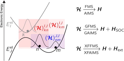13) ). Such interstate coupling terms are what accounts for the non-Born–Oppenheimer effects, that is, the fact that nuclear motion causes transfer of nuclear amplitude between electronic states. Figure 2 proposes a schematic representation of intrastate (blue) and interstate (red) couplings between TBFs in FMS.

Figure 2. Schematic representation of the different possible couplings between TBFs. Intrastate couplings are highlighted by a blue area, while interstates ones are depicted in red. The physics encapsulated in the Hamiltonian varies if one uses FMS/AIMS (molecular Hamiltonian – internal conversion), GFMS/GAIMS (molecular Hamiltonian plus spin–orbit coupling Hamiltonian – internal conversion and intersystem crossings) or XFFMS/XFAIMS (molecular Hamiltonian plus dipolar-coupling Hamiltonian – photo-triggered processes and internal conversion).

3.2.2. Spawning algorithm

One of the most important characteristics of the FMS strategy is its use of an adaptive basis set to describe nonadiabatic processes. As stated above, an FMS run starts with a linear combination of $N_{\mathrm{i}\mathrm{n}\mathrm{i}}$ coupled parent TBFs. In FMS, the number of TBFs describing the nuclear wavefunction in electronic state I will change over time due to so-called spawning events [134]. Each of the initial TBFs has the possibility to trigger the creation of new TBFs on coupled electronic states, whenever it evolves in regions characterised by a strong nonadiabaticity. At each step of the FMS dynamics, an effective nonadiabatic coupling between the state driving the TBF and all other electronic states is computed at the position of the TBF. This effective coupling is usually defined as the modulus of the nonadiabatic coupling vector, $|{\mathit{d}}_{IJ}|$, or the projection of the nonadiabatic coupling vector onto the classical velocity of the TBF, $|{\mathit{d}}_{IJ}\cdot \dot{\phantom{a}}{\overline{\mathit{R}}}_{k\text{β}}^{\left(I\right)}|$. If this effective coupling between the driving and any other electronic state at the current position of the TBF exceeds a predefined threshold, the propagation of the complex amplitudes is stopped and only the respective TBF is propagated until the point where a maximum in the effective coupling is reached. At this point, a new child TBF is spawned on the coupled state, if certain additional criteria are met [134,137,138]. In the case of a successful spawn, the child TBF with a complex amplitude of 0 and the parent TBF will be propagated back in time, until the time when the parent TBF entered into the coupling region. The FMS dynamics can then be resumed with the equations of motion defined by Equation (12(12) $\frac{\mathrm{d}{\mathit{C}}^I}{\mathrm{d}t}=-i\left({\mathit{S}}_{II}^{-1}\right)\left[\left({\mathit{H}}_{II}-i{\dot{\mathit{S}}}_{II}\right){\mathit{C}}^I+\sum _{J\ne I}^{\mathrm{\infty }}{\mathit{H}}_{IJ}{\mathit{C}}^J\right].$(12) ) extended by a new (child) TBF. The extended set of TBFs will allow for exchange of amplitude between the coupled electronic states. The spawning algorithm implies that the number of TBFs in state J (from branch β) in Equation (11(11) $\begin{array}{rl}\mathrm{\Psi }(\mathit{r},\mathit{R},t)& =\sum _{\text{β}}^{N_{\mathrm{i}\mathrm{n}\mathrm{i}}}{\tilde{\mathrm{\Psi }}}_{\text{β}}(\mathit{r},\mathit{R},t)\\ & =\sum _{\text{β}}^{N_{\mathrm{i}\mathrm{n}\mathrm{i}}}\sum _J^{\mathrm{\infty }}\sum _k^{N_{\mathrm{T}\mathrm{B}\mathrm{F}\mathrm{s}J,\text{β}}}{C}_{k\text{β}}^{\left(J\right)}\left(t\right){\tilde{\chi }}_{k\text{β}}^{\left(J\right)}\left(\mathit{R};{\overline{\mathit{R}}}_{k\text{β}}^{\left(J\right)}\left(t\right),{\overline{\mathit{P}}}_{k\text{β}}^{\left(J\right)}\left(t\right),{\overline{\gamma }}_{k\text{β}}^{\left(J\right)}\left(t\right),\mathit{\alpha }\right){\mathrm{\Phi }}_J(\mathit{r};\mathit{R}).\end{array}$(11) ) is actually time dependent: $N_{\mathrm{T}\mathrm{B}\mathrm{F}\mathrm{s}J,\text{β}}\to N_{\mathrm{T}\mathrm{B}\mathrm{F}\mathrm{s}J,\text{β}}\left(t\right)$. More details about the spawning algorithm can be found in Refs. [134,136,137,139].

3.2.3. Ab initio multiple spawning

The FMS framework described in the previous section would be in principle exact in the limit of a large number of TBFs and an exact evaluation of the matrix elements of its equations of motion (Equation 13(13) $\begin{array}{rl}& {\left(\mathit{H}\right)}_{k\text{β},k^{\prime }{\text{β}}^{\prime }}^{IJ}\\ & =⟨{\mathrm{\Phi }}_I{\tilde{\chi }}_{k\text{β}}^{\left(I\right)}|\hat{H}|{\tilde{\chi }}_{k^{\prime }{\text{β}}^{\prime }}^{\left(J\right)}{\mathrm{\Phi }}_J{⟩}_{\mathit{r},\mathit{R}}\\ & =⟨{\tilde{\chi }}_{k\text{β}}^{\left(I\right)}|{\hat{T}}_{\mathrm{N}}|{\tilde{\chi }}_{k^{\prime }{\text{β}}^{\prime }}^{\left(J\right)}{⟩}_{\mathit{R}}{\delta }_{IJ}+⟨{\tilde{\chi }}_{k\text{β}}^{\left(I\right)}|E_J^{\mathrm{e}\mathrm{l}}|{\tilde{\chi }}_{k^{\prime }{\text{β}}^{\prime }}^{\left(J\right)}{⟩}_{\mathit{R}}{\delta }_{IJ}\\ & -\sum _{\rho }^{3N_{\mathrm{N}}}\frac{1}{M_{\rho }}{⟨{\tilde{\chi }}_{k\text{β}}^{\left(I\right)}\left|{⟨{\mathrm{\Phi }}_I\left|\frac{\mathrm{\partial }}{\mathrm{\partial }{R}_{\rho }}\right|{\mathrm{\Phi }}_J⟩}_{\mathit{r}}\frac{\mathrm{\partial }}{\mathrm{\partial }{R}_{\rho }}\right|{\tilde{\chi }}_{k^{\prime }{\text{β}}^{\prime }}^{\left(J\right)}⟩}_{\mathit{R}}\\ & -\sum _{\rho }^{3N_{\mathrm{N}}}\frac{1}{2M_{\rho }}{⟨{\tilde{\chi }}_{k\text{β}}^{\left(I\right)}\left|{⟨{\mathrm{\Phi }}_I\left|\frac{{\mathrm{\partial }}^2}{\mathrm{\partial }{R}_{\rho }^2}\right|{\mathrm{\Phi }}_J⟩}_{\mathit{r}}\right|{\tilde{\chi }}_{k^{\prime }{\text{β}}^{\prime }}^{\left(J\right)}⟩}_{\mathit{R}}.\end{array}$(13) ). However, neither requirement can be strictly met if one is interested in the excited-state dynamics of molecules in their full dimensionality, and two key approximations have to be introduced and will define the AIMS method. These approximations are summarised below and the interested reader can consult Ref. [140] for their test and a more detailed discussion.

The Hamiltonian matrix elements described in Equation (13(13) $\begin{array}{rl}& {\left(\mathit{H}\right)}_{k\text{β},k^{\prime }{\text{β}}^{\prime }}^{IJ}\\ & =⟨{\mathrm{\Phi }}_I{\tilde{\chi }}_{k\text{β}}^{\left(I\right)}|\hat{H}|{\tilde{\chi }}_{k^{\prime }{\text{β}}^{\prime }}^{\left(J\right)}{\mathrm{\Phi }}_J{⟩}_{\mathit{r},\mathit{R}}\\ & =⟨{\tilde{\chi }}_{k\text{β}}^{\left(I\right)}|{\hat{T}}_{\mathrm{N}}|{\tilde{\chi }}_{k^{\prime }{\text{β}}^{\prime }}^{\left(J\right)}{⟩}_{\mathit{R}}{\delta }_{IJ}+⟨{\tilde{\chi }}_{k\text{β}}^{\left(I\right)}|E_J^{\mathrm{e}\mathrm{l}}|{\tilde{\chi }}_{k^{\prime }{\text{β}}^{\prime }}^{\left(J\right)}{⟩}_{\mathit{R}}{\delta }_{IJ}\\ & -\sum _{\rho }^{3N_{\mathrm{N}}}\frac{1}{M_{\rho }}{⟨{\tilde{\chi }}_{k\text{β}}^{\left(I\right)}\left|{⟨{\mathrm{\Phi }}_I\left|\frac{\mathrm{\partial }}{\mathrm{\partial }{R}_{\rho }}\right|{\mathrm{\Phi }}_J⟩}_{\mathit{r}}\frac{\mathrm{\partial }}{\mathrm{\partial }{R}_{\rho }}\right|{\tilde{\chi }}_{k^{\prime }{\text{β}}^{\prime }}^{\left(J\right)}⟩}_{\mathit{R}}\\ & -\sum _{\rho }^{3N_{\mathrm{N}}}\frac{1}{2M_{\rho }}{⟨{\tilde{\chi }}_{k\text{β}}^{\left(I\right)}\left|{⟨{\mathrm{\Phi }}_I\left|\frac{{\mathrm{\partial }}^2}{\mathrm{\partial }{R}_{\rho }^2}\right|{\mathrm{\Phi }}_J⟩}_{\mathit{r}}\right|{\tilde{\chi }}_{k^{\prime }{\text{β}}^{\prime }}^{\left(J\right)}⟩}_{\mathit{R}}.\end{array}$(13) ) imply the evaluation of integrals over all nuclear coordinates, with integrands containing electronic-structure quantities that precisely depend on the nuclear position. As such, computing Hamiltonian matrix elements in FMS requires a knowledge of these electronic-structure quantities at each possible nuclear configuration, implying the precomputation of all electronic-structure quantities over the entire nuclear configuration space. A strategy employed in AIMS to alleviate this issue is to approximate the integrals in the Hamiltonian elements. Let us consider that one wants to evaluate an integral between TBF k in state I and TBF $k^{\prime }$ in J with the generic electronic-structure quantity ${\theta }_{IJ}\left(\mathit{R}\right)=⟨{\mathrm{\Phi }}_I|\hat{\theta }\left(\mathit{R}\right)|{\mathrm{\Phi }}_J{⟩}_{\mathit{r}}$, (14) ${\left(\mathit{\theta }\right)}_{k\text{β},k^{\prime }{\text{β}}^{\prime }}^{IJ}=⟨{\tilde{\chi }}_{k\text{β}}^{\left(I\right)}|⟨{\mathrm{\Phi }}_I|\hat{\theta }|{\mathrm{\Phi }}_J{⟩}_{\mathit{r}}|{\tilde{\chi }}_{k^{\prime }{\text{β}}^{\prime }}^{\left(J\right)}{⟩}_{\mathit{R}}.$(14) One can start by expanding the electronic-structure quantity around the centroid position of the product of the two TBFs, ${\overline{\mathit{R}}}_{k\text{β},k^{\prime }{\text{β}}^{\prime }}^{\left(IJ\right)}=\frac{1}{2}({\overline{\mathit{R}}}_{k\text{β}}^{\left(I\right)}+{\overline{\mathit{R}}}_{k^{\prime }{\text{β}}^{\prime }}^{\left(J\right)})$: (15) $\begin{array}{rl}{\theta }_{IJ}\left(\mathit{R}\right)& ={\theta }_{IJ}\left({\overline{\mathit{R}}}_{k\text{β},k^{\prime }{\text{β}}^{\prime }}^{\left(IJ\right)}\right)\\ & +\sum _{\rho }^{3N_{\mathrm{N}}}(R_{\rho }-{\overline{R}}_{\rho ,k\text{β},k^{\prime }{\text{β}}^{\prime }}^{\left(IJ\right)}){\left.\frac{\mathrm{\partial }{\theta }_{IJ}\left(\mathit{R}\right)}{\mathrm{\partial }{R}_{\rho }}\right|}_{R_{\rho }={\overline{R}}_{\rho ,k\text{β},k^{\prime }{\text{β}}^{\prime }}^{\left(IJ\right)}}\\ & +\frac{1}{2}\sum _{\rho \tilde{\rho }}^{3N_{\mathrm{N}}}(R_{\rho }-{\overline{R}}_{\rho ,k\text{β},k^{\prime }{\text{β}}^{\prime }}^{\left(IJ\right)})\\ & \times {\left.\frac{{\mathrm{\partial }}^2{\theta }_{IJ}\left(\mathit{R}\right)}{\mathrm{\partial }{R}_{\rho }\mathrm{\partial }{R}_{\tilde{\rho }}}\right|}_{R_{\rho }={\overline{R}}_{\rho ,k\text{β},k^{\prime }{\text{β}}^{\prime }}^{\left(IJ\right)},R_{\tilde{\rho }}={\overline{R}}_{\tilde{\rho },k\text{β},k^{\prime }{\text{β}}^{\prime }}^{\left(IJ\right)}}\\ & \times (R_{\tilde{\rho }}-{\overline{R}}_{\tilde{\rho }k\text{β},k^{\prime }{\text{β}}^{\prime }}^{\left(IJ\right)})+\cdots \end{array}$(15) Considering the spatial localisation of the TBFs, the electronic-structure quantity of interest is assumed to be only slightly varying in the region of non-zero overlap between the two TBFs [134,139,141]. As a result, one assumes that the above Taylor expansion can be truncated after zeroth order, leading to the following (approximate) integrals: (16) $\begin{array}{rl}{\left(\mathit{\theta }\right)}_{k\text{β},k^{\prime }{\text{β}}^{\prime }}^{IJ}& =⟨{\tilde{\chi }}_{k\text{β}}^{\left(I\right)}|⟨{\mathrm{\Phi }}_I|\hat{\theta }|{\mathrm{\Phi }}_J{⟩}_{\mathit{r}}|{\tilde{\chi }}_{k^{\prime }{\text{β}}^{\prime }}^{\left(J\right)}{⟩}_{\mathit{R}}\\ & \approx {\theta }_{IJ}\left({\overline{\mathit{R}}}_{k\text{β},k^{\prime }{\text{β}}^{\prime }}^{\left(IJ\right)}\right)⟨{\tilde{\chi }}_{k\text{β}}^{\left(I\right)}|{\tilde{\chi }}_{k^{\prime }{\text{β}}^{\prime }}^{\left(J\right)}{⟩}_{\mathit{R}}.\end{array}$(16) Applying this so-called saddle-point approximation of order zero (SPA0) to the definition of the FMS Hamiltonian matrix elements (Equation 13(13) $\begin{array}{rl}& {\left(\mathit{H}\right)}_{k\text{β},k^{\prime }{\text{β}}^{\prime }}^{IJ}\\ & =⟨{\mathrm{\Phi }}_I{\tilde{\chi }}_{k\text{β}}^{\left(I\right)}|\hat{H}|{\tilde{\chi }}_{k^{\prime }{\text{β}}^{\prime }}^{\left(J\right)}{\mathrm{\Phi }}_J{⟩}_{\mathit{r},\mathit{R}}\\ & =⟨{\tilde{\chi }}_{k\text{β}}^{\left(I\right)}|{\hat{T}}_{\mathrm{N}}|{\tilde{\chi }}_{k^{\prime }{\text{β}}^{\prime }}^{\left(J\right)}{⟩}_{\mathit{R}}{\delta }_{IJ}+⟨{\tilde{\chi }}_{k\text{β}}^{\left(I\right)}|E_J^{\mathrm{e}\mathrm{l}}|{\tilde{\chi }}_{k^{\prime }{\text{β}}^{\prime }}^{\left(J\right)}{⟩}_{\mathit{R}}{\delta }_{IJ}\\ & -\sum _{\rho }^{3N_{\mathrm{N}}}\frac{1}{M_{\rho }}{⟨{\tilde{\chi }}_{k\text{β}}^{\left(I\right)}\left|{⟨{\mathrm{\Phi }}_I\left|\frac{\mathrm{\partial }}{\mathrm{\partial }{R}_{\rho }}\right|{\mathrm{\Phi }}_J⟩}_{\mathit{r}}\frac{\mathrm{\partial }}{\mathrm{\partial }{R}_{\rho }}\right|{\tilde{\chi }}_{k^{\prime }{\text{β}}^{\prime }}^{\left(J\right)}⟩}_{\mathit{R}}\\ & -\sum _{\rho }^{3N_{\mathrm{N}}}\frac{1}{2M_{\rho }}{⟨{\tilde{\chi }}_{k\text{β}}^{\left(I\right)}\left|{⟨{\mathrm{\Phi }}_I\left|\frac{{\mathrm{\partial }}^2}{\mathrm{\partial }{R}_{\rho }^2}\right|{\mathrm{\Phi }}_J⟩}_{\mathit{r}}\right|{\tilde{\chi }}_{k^{\prime }{\text{β}}^{\prime }}^{\left(J\right)}⟩}_{\mathit{R}}.\end{array}$(13) ) yields, after neglecting the second-order couplings, the AIMS Hamiltonian matrix elements: (17) $\begin{array}{rl}{\left(\mathit{H}\right)}_{k\text{β},k^{\prime }{\text{β}}^{\prime }}^{IJ}& \approx ⟨{\tilde{\chi }}_{k\text{β}}^{\left(I\right)}|{\hat{T}}_{\mathrm{N}}|{\tilde{\chi }}_{k^{\prime }{\text{β}}^{\prime }}^{\left(J\right)}{⟩}_{\mathit{R}}{\delta }_{IJ}\\ & +E_J^{\mathrm{e}\mathrm{l}}\left({\overline{\mathit{R}}}_{k\text{β},k^{\prime }{\text{β}}^{\prime }}^{\left(IJ\right)}\right)⟨{\tilde{\chi }}_{k\text{β}}^{\left(I\right)}|{\tilde{\chi }}_{k^{\prime }{\text{β}}^{\prime }}^{\left(J\right)}{⟩}_{\mathit{R}}{\delta }_{IJ}\\ & -\sum _{\rho }^{3N_{\mathrm{N}}}\frac{1}{M_{\rho }}{\left({\mathit{d}}_{IJ}\left({\overline{\mathit{R}}}_{k\text{β},k^{\prime }{\text{β}}^{\prime }}^{\left(IJ\right)}\right)\right)}_{\rho }\\ & \times ⟨{\tilde{\chi }}_{k\text{β}}^{\left(I\right)}\left|\frac{\mathrm{\partial }}{\mathrm{\partial }{R}_{\rho }}\right|{\tilde{\chi }}_{k^{\prime }{\text{β}}^{\prime }}^{\left(J\right)}{⟩}_{\mathit{R}}.\end{array}$(17) Calculating Hamiltonian matrix elements using the saddle-point approximation of order zero allows for the on-the-fly propagation of the AIMS equations of motion. TBFs are propagated based on ab initio molecular dynamics, while the equations for the complex amplitudes (Equation 12(12) $\frac{\mathrm{d}{\mathit{C}}^I}{\mathrm{d}t}=-i\left({\mathit{S}}_{II}^{-1}\right)\left[\left({\mathit{H}}_{II}-i{\dot{\mathit{S}}}_{II}\right){\mathit{C}}^I+\sum _{J\ne I}^{\mathrm{\infty }}{\mathit{H}}_{IJ}{\mathit{C}}^J\right].$(12) ) require additional electronic-structure calculations at the centroid position between each pair of TBFs, coupling them together.

The second approximation is the so-called independent first generation approximation (IFGA). In FMS, the dynamics is usually initialised with a linear combination of $N_{\mathrm{i}\mathrm{n}\mathrm{i}}$ coupled parent TBFs mimicking an initial nuclear wavepacket. In the high-dimensional case of a molecule, a nuclear wavepacket is expected to rapidly spread in configuration space after photoexcitation, hence the initial parent TBFs are expected to uncouple rapidly and, as a result, evolve independently shortly after the beginning of the dynamics. Within the framework of the IFGA, the initial parent TBFs are considered uncoupled from the very beginning of the dynamics [133,134]. Within the IFGA, one can sample the initial conditions for each parent TBF from a Wigner distribution and run them independently. Consequently, it is assumed that all TBFs from a branch β will evolve completely independently from any TBFs coming from a different branch ${\text{β}}^{\prime }$.

Applying the SPA0 and the IFGA to the FMS equations of motion leads to the AIMS method,³ which allows for the description of the nonadiabatic dynamics of molecules in full dimensionality. AIMS has been successfully employed to elucidate the photochemistry of numerous molecules (see Refs. [7,117,119,143–147] for example and Refs. [136,148] for a more detailed list of applications).

3.2.4. Extension of full- and ab initio multiple spawning

The FMS equations of motion introduced above describe the nonadiabatic dynamics of a molecule in an in principle exact way under the assumption that such excited-state dynamics can be fully described by the molecular Hamiltonian given in Equation (2(2) $\begin{array}{rl}\hat{H}(\mathit{r},\mathit{R})& =-\sum _{\gamma }^{N_{\mathrm{N}}}\frac{1}{2M_{\gamma }}{\mathrm{\nabla }}_{\gamma }^2-\sum _i^{N_{\mathrm{e}\mathrm{l}}}\frac{1}{2}{\mathrm{\nabla }}_i^2+\sum _{i<j}\frac{1}{|{\mathit{r}}_i-{\mathit{r}}_j|}\\ & -\sum _{\gamma ,i}\frac{Z_{\gamma }}{|{\mathit{R}}_{\gamma }-{\mathit{r}}_i|}+\sum _{\gamma <\text{β}}\frac{Z_{\gamma }{Z}_{\text{β}}}{|{\mathit{R}}_{\gamma }-{\mathit{R}}_{\text{β}}|}\\ & =-\sum _{\gamma }^{N_{\mathrm{N}}}\frac{1}{2M_{\gamma }}{\mathrm{\nabla }}_{\gamma }^2+{\hat{\mathcal{H}}}_{\mathrm{e}\mathrm{l}}(\mathit{r},\mathit{R})\\ & ={\hat{T}}_{\mathrm{N}}\left(\mathit{R}\right)+{\hat{\mathcal{H}}}_{\mathrm{e}\mathrm{l}}(\mathit{r},\mathit{R}).\end{array}$(2) ) (Figure 2). Hence, the FMS framework described until now only allows for the description of nonradiative deexcitation of molecules via internal conversion pathways (events 4 and 6 in Figure 1). As indicated earlier, other physical processes related to excited states can be of importance like intersystem crossings (event 5 in Figure 1) or the explicit interaction of a molecule with an external electromagnetic field to produce photoexcitation (event 2 in Figure 1) or phototriggered processes. The description of such events can easily be included within an FMS (or AIMS) framework by adding the necessary supplementary terms to the molecular Hamiltonian, leading to additional couplings between the TBFs resulting from the presence of extra physical processes (in the following, we denote the modified molecular Hamiltonian by $\hat{\mathcal{H}}$).

In the Generalised FMS method (GFMS) [149], a spin–orbit coupling Hamiltonian [150,151] is added to the molecular Hamiltonian: (18) $\hat{\mathcal{H}}(\mathit{x},\mathit{R})=\hat{H}(\mathit{r},\mathit{R})+{\hat{H}}_{\mathrm{S}\mathrm{O}\mathrm{C}}(\mathit{x},\mathit{R}),$(18) where $\mathit{x}=(\mathit{r},s)$ (we indicate here the spin component for the electronic degrees of freedom only). Thanks to this additional term and an alteration of the spawning algorithm, GFMS (and its approximate version GAIMS) can be used to describe internal conversion and intersystem crossing events on an equal footing. An alternative implementation of spin–orbit coupling in FMS is presented in Refs. [152,153].

In the eXternal Field FMS (XFFMS or XFAIMS in its AIMS approximation) [154], the molecular Hamiltonian is supplemented by a dipolar coupling term, allowing for couplings between TBFs mediated by an external electromagnetic field $\underset{\_}{\mathit{E}}\left(t\right)$ (an underlined bold symbol indicates a 3D vector): (19) $\hat{\mathcal{H}}(\mathit{r},\mathit{R},t)=\hat{H}(\mathit{r},\mathit{R})-\underset{\_}{\hat{\mathit{\mu }}}(\mathit{r},\mathit{R})\cdot \underset{\_}{\mathit{E}}\left(t\right),$(19) where $\underset{\_}{\hat{\mathit{\mu }}}(\mathit{r},\mathit{R})={\underset{\_}{\hat{\mathit{\mu }}}}^{\mathrm{e}\mathrm{l}}\left(\mathit{r}\right)+{\underset{\_}{\hat{\mathit{\mu }}}}^{\mathrm{N}}\left(\mathit{R}\right)$ is the molecular dipole moment, composed of an electronic and a nuclear part. Photo(de)excitation processes with laser pulses as well as more complex in silico experiments like pump-dump [155] or control [156] can be achieved within this framework. The effect of an external field in FMS has also been included in a Floquet-type approach [157,158].

Figure 2 summarises the different types of couplings in FMS (AIMS) and its extensions.

3.3. Trajectory surface hopping

TSH belongs to the family of mixed quantum/classical methods for nonadiabatic dynamics [159]. TSH proposes to portray the nonadiabatic dynamics of nuclear wavepackets by using swarms of independent classical trajectories – within the so-called independent trajectory approximation (ITA) – that can hop from one electronic state to the other in case of strong nonadiabaticity [35,160].

In TSH, the nuclei of a molecule are propagated classically based on Newton's equations of motion. Hence, the nuclear force felt by the molecule at time t along a certain trajectory, labelled α, is given by (20) ${\mathbf{F}}^{\alpha }\left(t\right)=-{\mathbf{\nabla }}_{\mathit{R}}{E}_{\ast }^{\mathrm{e}\mathrm{l}}\left(\mathit{R}\right){|}_{\mathit{R}={\mathit{R}}^{\alpha }\left(t\right)}.$(20) The notation $E_{\ast }^{\mathrm{e}\mathrm{l}}\left(\mathit{R}\right)$ indicates that the classical force is obtained from a given (adiabatic) electronic state that can change during the dynamics to reproduce nonadiabatic transitions. How can the driving state of the dynamics at each nuclear time step be determined? Tully proposed an algorithm, coined Fewest Switches, which limits the number of hopping events to a minimum in a TSH run [37]. (In the following, we will use the acronym TSH to denote surface hopping within the fewest switches algorithm.) Each trajectory α is assigned a time-dependent electronic wavefunction given by (21) $\tilde{\mathrm{\Phi }}(\mathit{r};{\mathit{R}}^{\alpha },t)=\sum _I{c}_I^{\alpha }\left(t\right){\mathrm{\Phi }}_I(\mathit{r};{\mathit{R}}^{\alpha }),$(21) with ${\mathrm{\Phi }}_I(\mathit{r};{\mathit{R}}^{\alpha })$ being a solution of the time-independent Schrödinger equation (3(3) ${\hat{\mathcal{H}}}_{\mathrm{e}\mathrm{l}}(\mathit{r},\mathit{R}){\mathrm{\Phi }}_J(\mathit{r};\mathit{R})=E_J^{\mathrm{e}\mathrm{l}}\left(\mathit{R}\right){\mathrm{\Phi }}_J(\mathit{r};\mathit{R}),$(3) ) for nuclear configuration $\mathit{R}={\mathit{R}}^{\alpha }\left(t\right)$, and $c_I^{\alpha }\left(t\right)$ a set of complex coefficients. A set of equations of motion for the complex amplitudes can be obtained by inserting Equation (21(21) $\tilde{\mathrm{\Phi }}(\mathit{r};{\mathit{R}}^{\alpha },t)=\sum _I{c}_I^{\alpha }\left(t\right){\mathrm{\Phi }}_I(\mathit{r};{\mathit{R}}^{\alpha }),$(21) ) into the time-dependent electronic Schrödinger equation (plus some algebra), (22) ${\dot{c}}_J^{\alpha }\left(t\right)=-i{E}_J^{\mathrm{e}\mathrm{l}}\left({\mathit{R}}^{\alpha }\right)c_J^{\alpha }\left(t\right)-\sum _I{\dot{\mathit{R}}}^{\alpha }\left(t\right)\cdot {\mathit{d}}_{JI}\left({\mathit{R}}^{\alpha }\right)c_I^{\alpha }\left(t\right).$(22) We note the presence of the nonadiabatic coupling vectors ${\mathit{d}}_{JI}\left({\mathit{R}}^{\alpha }\right)$ in Equation (22(22) ${\dot{c}}_J^{\alpha }\left(t\right)=-i{E}_J^{\mathrm{e}\mathrm{l}}\left({\mathit{R}}^{\alpha }\right)c_J^{\alpha }\left(t\right)-\sum _I{\dot{\mathit{R}}}^{\alpha }\left(t\right)\cdot {\mathit{d}}_{JI}\left({\mathit{R}}^{\alpha }\right)c_I^{\alpha }\left(t\right).$(22) ), which are projected onto the nuclear velocity vector (at time t), ${\dot{\mathit{R}}}^{\alpha }\left(t\right)$.

A TSH run typically starts by selecting the initial conditions (positions and momenta) for a given trajectory α and the initial driving state. At time $t_0$, all the complex coefficients are set to zero, except for the one corresponding to the initial driving state which is initiated to one. The nuclear degrees of freedom are propagated according to Equation (20(20) ${\mathbf{F}}^{\alpha }\left(t\right)=-{\mathbf{\nabla }}_{\mathit{R}}{E}_{\ast }^{\mathrm{e}\mathrm{l}}\left(\mathit{R}\right){|}_{\mathit{R}={\mathit{R}}^{\alpha }\left(t\right)}.$(20) ), with the electronic energy being that of the initial state. After each nuclear integration time step, (i) the amplitudes are propagated (with a smaller time step) based on Equation (22(22) ${\dot{c}}_J^{\alpha }\left(t\right)=-i{E}_J^{\mathrm{e}\mathrm{l}}\left({\mathit{R}}^{\alpha }\right)c_J^{\alpha }\left(t\right)-\sum _I{\dot{\mathit{R}}}^{\alpha }\left(t\right)\cdot {\mathit{d}}_{JI}\left({\mathit{R}}^{\alpha }\right)c_I^{\alpha }\left(t\right).$(22) ), (ii) a probability for the trajectory α to jump from the driving electronic state to another one is computed and (iii) a stochastic algorithm is employed to determine whether the trajectory should change state. The fewest-switches probability to hop from state J to any other electronic state I between time t and $t+\mathrm{d}t$ is given by [37], (23) $\begin{array}{rl}{\mathcal{P}}_{J\to I}^{\alpha }& =max\left[0,\frac{-2\mathrm{d}t}{{\left|c_J^{\alpha }\left(t\right)\right|}^2}\mathrm{\Re }\left[c_J^{\alpha \ast }\left(t\right)c_I^{\alpha }\left(t\right)\right]{\dot{\mathit{R}}}^{\alpha }\left(t\right)\right.\\ & \cdot \left.{\mathit{d}}_{IJ}\left({\mathit{R}}^{\alpha }\right)\phantom{\frac{-2\mathrm{d}t}{{\left|c_J^{\alpha }\left(t\right)\right|}^2}}\right].\end{array}$(23) A hop occurs from J to another electronic state I if (24) $\sum _K^{I-1}{\mathcal{P}}_{J\to K}^{\alpha }\le \zeta \le \sum _K^I{\mathcal{P}}_{J\to K}^{\alpha },$(24) where ζ is a random number generated uniformly in the interval $[0:1]$. The trajectory is propagated until the predetermined completion criterion. This summarises the main steps for the propagation of a single trajectory α, but it is critical to realise that a large number of independent trajectories, or independent TSH runs, are required to converge the hopping algorithm and the sampling of initial conditions. We note that new flavours of TSH have recently been proposed [161].

3.4. Ab initio multiple spawning vs trajectory surface hopping

In the following, we aim at comparing the two different ansätze for nonadiabatic dynamics proposed by TSH and AIMS. To achieve this goal, it is necessary to compare the respective equations of motion for the complex amplitudes. Let us consider a system consisting of two electronic states I and J.

In TSH the equations of motion for a certain trajectory α read (25) $\left(\begin{array}{c}{\dot{c}}_I^{\alpha }\left(t\right)\\ {\dot{c}}_J^{\alpha }\left(t\right)\end{array}\right)=-i\left(\begin{array}{cc}{H}_{II}^{\alpha }& H_{IJ}^{\alpha }\\ H_{JI}^{\alpha }& H_{JJ}^{\alpha }\end{array}\right)\left(\begin{array}{c}{c}_I^{\alpha }\left(t\right)\\ c_J^{\alpha }\left(t\right)\end{array}\right),$(25) with the Hamiltonian elements being defined as $H_{II}^{\alpha }=E_I\left({\mathit{R}}^{\alpha }\right)$ and $H_{IJ}^{\alpha }=-i{\mathit{d}}_{IJ}\left({\mathit{R}}^{\alpha }\right)\cdot \dot{\phantom{a}}{\mathit{R}}^{\alpha }\left(t\right)$ following Equation (22(22) ${\dot{c}}_J^{\alpha }\left(t\right)=-i{E}_J^{\mathrm{e}\mathrm{l}}\left({\mathit{R}}^{\alpha }\right)c_J^{\alpha }\left(t\right)-\sum _I{\dot{\mathit{R}}}^{\alpha }\left(t\right)\cdot {\mathit{d}}_{JI}\left({\mathit{R}}^{\alpha }\right)c_I^{\alpha }\left(t\right).$(22) ).

In AIMS, assuming the simple case of two TBFs evolving on state I and one TBF on state J, we will obtain the following equations of motion: (26) $\begin{array}{rl}& \left(\begin{array}{ccc}{S}_{11}^{II}& S_{12}^{II}& 0\\ S_{21}^{II}& S_{22}^{II}& 0\\ 0& 0& S_{11}^{JJ}\end{array}\right)\left(\begin{array}{c}{\dot{C}}_1^I\left(t\right)\\ {\dot{C}}_2^I\left(t\right)\\ {\dot{C}}_1^J\left(t\right)\end{array}\right)\\ & =-i\left[\left(\begin{array}{ccc}{H}_{11}^{II}& H_{12}^{II}& H_{11}^{IJ}\\ H_{21}^{II}& H_{22}^{II}& H_{21}^{IJ}\\ H_{11}^{JI}& H_{12}^{JI}& H_{11}^{JJ}\end{array}\right)\right.\\ & -\left.i\left(\begin{array}{ccc}{\dot{S}}_{11}^{II}& {\dot{S}}_{12}^{II}& 0\\ {\dot{S}}_{21}^{II}& {\dot{S}}_{22}^{II}& 0\\ 0& 0& {\dot{S}}_{11}^{II}\end{array}\right)\right]\left(\begin{array}{c}{C}_1^I\left(t\right)\\ C_2^I\left(t\right)\\ C_1^J\left(t\right)\end{array}\right)\end{array}$(26) with the Hamiltonian matrix elements being defined as $H_{k{k}^{\prime }}^{II}=E_I^{\mathrm{e}\mathrm{l}}\left({\overline{\mathit{R}}}_{k{k}^{\prime }}^{\left(II\right)}\right(t\left)\right)⟨{\tilde{\chi }}_k^{\left(I\right)}|{\tilde{\chi }}_{k^{\prime }}^{\left(I\right)}{⟩}_{\mathit{R}}$ and $H_{k{k}^{\prime }}^{IJ}=-\sum _{\rho }^{3N_{\mathrm{N}}}\left(1/M_{\rho }\right)\left({\mathit{d}}_{IJ}\right({\overline{\mathit{R}}}_{k,k^{\prime }}^{\left(IJ\right)}){)}_{\rho }⟨{\tilde{\chi }}_k^{\left(I\right)}|\mathrm{\partial }/\mathrm{\partial }{R}_{\rho }|{\tilde{\chi }}_{k^{\prime }}^{\left(J\right)}{⟩}_{\mathit{R}}$.

Comparing these two sets of equations of motion clearly highlights the difference between the ITA inherent to TSH and the coupled TBFs strategy employed by AIMS. As a consequence of the ITA, all inter- and intrastate interactions between different trajectories are neglected within TSH, and interstate couplings are exclusively evaluated at the location of the trajectory α at time t. Which kind of approximations shall we perform on the AIMS matrix elements to bridge the equations of motion of AIMS to those of TSH? The most obvious approximation is to set the overlap and Hamiltonian matrix elements of the type ${\dot{S}}_{k{k}^{\prime }}^{II}$ and $H_{k{k}^{\prime }}^{II}$ to zero in Equation (26(26) $\begin{array}{rl}& \left(\begin{array}{ccc}{S}_{11}^{II}& S_{12}^{II}& 0\\ S_{21}^{II}& S_{22}^{II}& 0\\ 0& 0& S_{11}^{JJ}\end{array}\right)\left(\begin{array}{c}{\dot{C}}_1^I\left(t\right)\\ {\dot{C}}_2^I\left(t\right)\\ {\dot{C}}_1^J\left(t\right)\end{array}\right)\\ & =-i\left[\left(\begin{array}{ccc}{H}_{11}^{II}& H_{12}^{II}& H_{11}^{IJ}\\ H_{21}^{II}& H_{22}^{II}& H_{21}^{IJ}\\ H_{11}^{JI}& H_{12}^{JI}& H_{11}^{JJ}\end{array}\right)\right.\\ & -\left.i\left(\begin{array}{ccc}{\dot{S}}_{11}^{II}& {\dot{S}}_{12}^{II}& 0\\ {\dot{S}}_{21}^{II}& {\dot{S}}_{22}^{II}& 0\\ 0& 0& {\dot{S}}_{11}^{II}\end{array}\right)\right]\left(\begin{array}{c}{C}_1^I\left(t\right)\\ C_2^I\left(t\right)\\ C_1^J\left(t\right)\end{array}\right)\end{array}$(26) ). This will uncouple the TBFs evolving on the same state and prevent amplitude transfer between them. Recovering the interstate couplings of TSH from the AIMS equations would in addition require that the two coupled TBFs, evolving on different electronic states, follow the same trajectory, leading to a perfect overlap between them at all time.

While the ITA greatly simplifies the TSH algorithm and allows for a computational cost scaling linearly with the number of TSH trajectories, it is clear from the previous analysis that the trajectories produced might suffer from potential artefacts. In particular, the original TSH struggles in cases where the nuclear wavepacket branches in a nonadiabatic region, leading to a separation of the nuclear components on the two coupled surfaces – a phenomena often coined decoherence. The fact that the TSH complex amplitudes are evolved on the support of a single trajectory implies that a TSH trajectory can become overcoherent, that is, complex coefficients cannot decohere from each other, being forced to follow a single trajectory [162–169]. This is in stark contrast with AIMS, where the use of coupled TBFs, possibly evolving on different electronic states, allows for the description of wavepacket branchings.

3.4.1. Decoherence in trajectory surface hopping and ab initio multiple spawning for molecular systems

While TSH in its original version lacks the possibility to describe decoherence effects, different corrections to its formalism have been proposed to improve its result [170–176]. One of the simplest and most widely used methods is coined energy-based decoherence correction (EDC) and was proposed by Granucci and Persico [163]. This strategy aims at restoring the internal consistency of TSH [163]: the fraction of trajectories in an electronic state I at time t, ${\mathrm{\Pi }}_I\left(t\right)=N_I\left(t\right)/N_{\mathrm{t}\mathrm{r}\mathrm{a}\mathrm{j}}$, should be equal to the averaged electronic population in an electronic state I at time t, ${\overline{p}}_I\left(t\right)=\left(1/N_{\mathrm{t}\mathrm{r}\mathrm{a}\mathrm{j}}\right)\sum _{\alpha }^{N_{\mathrm{t}\mathrm{r}\mathrm{a}\mathrm{j}}}|c_I^{\alpha }\left(t\right){|}^2$, for all I and t. Based on earlier work by Truhlar and coworkers in the context of mean-field methods [177,178], the idea of the EDC is to exponentially dampen the population of the inactive TSH states at each time step, using as a damping time a function depending on the energy difference between each inactive state and the active one. Considering a TSH trajectory with active electronic state I, the complex amplitudes would be corrected after each TSH integration step using the following prescriptions: (27) $\begin{array}{rl}{c}_J^{{}^{\prime }\alpha }\left(t\right)& =c_J^{\alpha }\left(t\right)\exp (-\mathrm{\Delta }t/{\tau }_{IJ}^{\alpha }),\mathrm{\forall }J\ne I,\\ c_I^{{}^{\prime }\alpha }\left(t\right)& =c_I^{\alpha }\left(t\right){\left[\frac{1-\sum _{J\ne I}|c_J^{{}^{\prime }\alpha }\left(t\right){|}^2}{|c_I^{\alpha }\left(t\right){|}^2}\right]}^{1/2},\\ {\tau }_{IJ}^{\alpha }& =\frac{\hslash }{|E_J^{\mathrm{e}\mathrm{l},\alpha }-E_I^{\mathrm{e}\mathrm{l},\alpha }|}\left(1+\frac{\mathcal{C}}{E_{\mathrm{k}\mathrm{i}\mathrm{n}}^{\alpha }}\right),\end{array}$(27) with $E_{\mathrm{k}\mathrm{i}\mathrm{n}}^{\alpha }$ being the nuclear kinetic energy of the TSH trajectory α at time t and $\mathcal{C}$ a constant. Zhu et al. observed that their results were quite insensitive to the parameter $\mathcal{C}$ [177] and used a value of 0.1 hartree. This value has been used and tested in the context of TSH [163] and became the usual default value for $\mathcal{C}$ in most applications of the EDC for molecular systems. Other more involved correction schemes have been introduced in the literature, like the (parameter-free) augmented fewest switches surface hopping (A-FSSH) strategy proposed by Subotnik and coworkers [175,179,180].

These different decoherence-correction strategies have been extensively tested on a variety of model systems, where an uncorrected TSH dynamics would break down, and showed to provide reasonable corrections (see, e.g. [163,171,175,176,179,181,182]).

It is interesting to note, however, that only a few works have been highlighting the role of such decoherence correction for the nonadiabatic dynamics of molecules (see, e.g. [171,183–186]). In the following, we introduce some preliminary calculations aiming at assessing the role of a decoherence correction (EDC) in TSH for the molecule DMABN, and comparing the outcome of TSH dynamics with the one of AIMS. DMABN is a molecule famous for its dual fluorescence. Its ultrafast dynamics upon photoexcitation in the second excited electronic state (S${}_2$) has been recently studied using TSH/LR-TDDFT [187], TSH/ADC(2) [188], A-FSSH/LR-TDDFT [189] and AIMS/LR-TDDFT [118]. All methods describe an ultrafast relaxation of the S${}_2$ population towards S${}_1$ in less than 50 fs, without a twist of the dimethylamino group (as proposed in an earlier theoretical work [190]). Such an ultrafast decay from S${}_2$ was also observed for a parent molecule, 4-aminobenzonitrile, using the quantum dynamics method ML-MCTDH [191]. Interestingly, both TSH/ADC(2) and AIMS/LR-TDDFT nonadiabatic dynamics show that, while the nuclear wavepacket formed on S${}_2$ rapidly transfers amplitude towards S${}_1$, some population also moves back from S${}_1$ to S${}_2$ at later times. This observation is quite important in the context of TSH, as such oscillations of population between two states (or the presence of a non-zero nonadiabatic coupling for an extended period of time) can lead to a decoherence problem with an uncorrected TSH [171]. As such, DMABN constitutes a molecular example of the Tully Model II [37].

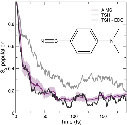
Using a common set of initial conditions, two TSH dynamics were conducted for the DMABN molecule: one with a decoherence correction (TSH-EDC) and one without.⁴ The difference in the population decay between the two TSH dynamics is striking (Figure 3, dark and light grey curves). The S${}_2$ population trace obtained with TSH-EDC shows a faster decay than TSH and exhibits less oscillations. Internal consistency is only fulfilled in the TSH dynamics including EDC. More importantly, TSH-EDC is in good agreement with the AIMS/LR-TDDFT result, showing as expected that AIMS naturally accounts for decoherence effects thanks to its use of coupled TBFs. We note that a previous comparison of A-FSSH/LR-TDDFT with TSH/LR-TDDFT (supporting information of  [189]) did not show such a pronounced difference between the dynamics with and without a correction. These simulations, however, used a different way of sampling initial conditions (initial conditions sampled from a ground-state ab initio molecular dynamics) and showed no residual S${}_2$ population after 50 fs of dynamics, in contrast to the other TSH and AIMS simulations.

Figure 3. Preliminary results on the nonadiabatic molecular dynamics of the molecule DMABN (inset). The population trace of the initially photoexcited state S${}_2$ molecule is plotted over time for TSH (light grey), TSH with the decoherence correction ‘EDC’ (dark grey) and AIMS (palatinate).

While the corrections described above can provide an ad hoc way of correcting TSH for the problem of decoherence, it is important to realise that they do not alleviate all the issues related to the use of independent trajectories. Nonadiabatic interferences between nuclear wavepackets on different electronic states are notorious for triggering a breakdown of the ITA (see, e.g. [148,165,180,195,196]), which cannot be easily fixed by a decoherence corrections [197]. The explicit simulation of photoexcitation processes or pump/probe dynamics in TSH can also become problematic in certain regimes [198], and XFAIMS constitutes an appealing alternative for such cases [199].

4. An alternative perspective on nonadiabatic dynamics

Up to this point, all concepts and methods discussed emerged from a Born–Huang picture of the molecular wavefunction, i.e. the molecular wavefunction is represented by Equation (4(4) $\mathrm{\Psi }(\mathit{r},\mathit{R},t)=\sum _J^{\mathrm{\infty }}{\mathrm{\Phi }}_J(\mathit{r};\mathit{R}){\chi }_J(\mathit{R},t).$(4) ). As discussed above, this representation is the cornerstone for our way of thinking about excited-state dynamics as nuclear wavepackets evolving on electronic eigenstates. It is, however, important to keep in mind that Born–Huang is only one of the possible representations of $\mathrm{\Psi }(\mathit{r},\mathit{R},t)$, and adopting a different viewpoint would lead to a change of perspective in our way of describing photochemistry and photophysics. Consider, for example, that we do not perform an expansion in an electronic basis, but instead use a time-dependent electronic wavefunction with a parametric dependence on the nuclear coordinates. Within this proposition, the molecular wavefunction would be represented by (28) $\mathrm{\Psi }(\mathit{r},\mathit{R},t)=\chi (\mathit{R},t)\mathrm{\Phi }(\mathit{r};\mathit{R},t),$(28) where $\chi (\mathit{R},t)$ is the time-dependent nuclear wavefunction and $\mathrm{\Phi }(\mathit{r};\mathit{R},t)$ the time-dependent electronic wavefunction. Such a representation of the molecular wavefunction can be shown to be exact when supplemented with a partial normalisation condition $\int \mathrm{d}\mathit{r}|\mathrm{\Phi }(\mathit{r};\mathit{R},t){|}^2=1$ $\mathrm{\forall }\mathit{R},t$, and has been coined Exact Factorisation [62,200–203]. The representation in Equation (28(28) $\mathrm{\Psi }(\mathit{r},\mathit{R},t)=\chi (\mathit{R},t)\mathrm{\Phi }(\mathit{r};\mathit{R},t),$(28) ) is a generalisation of the time-independent factorisation proposed earlier by Hunter [204–208]. We note that the importance of the parametric dependence in the electronic wavefunction on the nuclear coordinates has been discussed in Ref. [209].

How does the Exact Factorisation representation of the molecular wavefunction differ from the Born–Huang one? Equations of motion for the nuclear and electronic time-dependent wavefunctions – obtained upon insertion of Equation (28(28) $\mathrm{\Psi }(\mathit{r},\mathit{R},t)=\chi (\mathit{R},t)\mathrm{\Phi }(\mathit{r};\mathit{R},t),$(28) ) into the time-dependent Schrödinger equation and using the partial normalisation condition, see Refs. [202] for details – reveal a rather different picture of nonadiabatic phenomena. The concept of multiple time-independent electronic eigenstates disappears, as does the idea that a series of coupled nuclear amplitudes are evolving on different static PESs. Instead, the Exact Factorisation proposes to picture the dynamics of a molecule in the excited state as a single time-dependent nuclear wavefunction evolving under the action of a single time-dependent potential energy surface and a single time-dependent vector potential [210]. The behaviour of these time-dependent potentials has been studied in details for model systems [202,211], and it was shown for example that propagating independent classical trajectories with forces derived from the time-dependent PES already offers an excellent approximation to the nuclear wavepacket dynamics [212,213], even in cases of nonadiabatic interferences [196]. As the nuclei only have to follow a single time-dependent PES, no hopping or spawning is required in stark contrast to the Born–Huang representation. These observations greatly motivated the development of approximate nonadiabatic dynamics strategies based on the Exact Factorisation [62,214,215], with methods like the coupled-trajectory mixed quantum/classical (CT-MQC) strategy having been applied to the excited-state dynamics of molecular systems [216–221]. The Exact Factorisation has also been used to shed new lights on the dynamics through conical intersections [222,223] – conical intersections being related to a Born–Huang expansion in adiabatic electronic states – as well as the geometric phase [224]. Figure 4 presents, for a two-dimensional model system, a comparison between the potential energy surfaces and nonadiabatic coupling vectors obtained within the Born–Huang representation (Figure 4a) and a snapshot of the corresponding Exact-Factorisation quantities – time-dependent potential energy surface and vector potential – at the time when the nuclear wavefunction hits the nonadiabatic region (Figure 4b) (see Ref. [223] for more details). The time-dependent potential energy surface and vector potential are smooth and do not exhibit the typical features of the corresponding adiabatic ( Born–Huang) quantities.

Figure 4. Two-dimensional nonadiabatic model system. (a) Born–Huang representation: potential energy surfaces exhibiting a conical intersection (surface plots) and corresponding nonadiabatic coupling vectors (arrows, as unit vectors) for a model system in the adiabatic representation. (b) Exact-Factorisation representation: the surface represents the gauge-independent contribution to the time-dependent PES and the arrows the time-dependent vector potential at the time when the nuclear wavefunction, in the Born–Huang simulation, passes through the conical intersection. Figure based on the results published in  [223].

5. Summary

The use of TBFs to perform excited-state dynamics has been stimulated by recent progress within the frameworks of AIMS, MCE or vMCG. In this New Views article, we discussed the details of the former strategy as well as its recent developments. We also proposed a comparison of AIMS with the most commonly employed techniques to perform nonadiabatic molecular dynamics, TSH, for cases where decoherence between nuclear wavepackets can play a role. Dramatic improvement in the efficiency of electronic structure methods will surely be a key ingredient for a more general use of TBFs-based nonadiabatic methods, and recent developments in the field appear to be very promising. New routes to solve the time-dependent molecular Schrödinger equation will perhaps emerge from the Exact Factorisation – for example a scheme combining TBFs within a vMCG framework, Ehrenfest dynamics, and the Exact Factorisation has recently been developed for excited-state dynamics [225]. The study of photochemistry in optical cavity (or emission processes) will most likely become another important line of research for TBFs-based strategies, as recently done with other techniques [226–228].

Disclosure statement

No potential conflict of interest was reported by the authors.

Additional information

Funding

This project has received funding from the H2020 European Research Council European Union's Horizon 2020 research and innovation programme under grant agreement No 803718 (SINDAM). LMI acknowledges the EPSRC for an EPSRC Doctoral Studentship (EP/R513039/1).

Notes

1. We note that on-the-fly diabatisation is possible, see, e.g. [115,116].

2. Kasha's rule suggests that the excited electronic state from which luminescence takes place is often the lowest one.

3. We note that the total (classical) energy for each individual TBF is strictly conserved and used in simulations to detect any potential issue with the underlying electronic structure calculations. From a quantum perspective, while the norm of the total wavefunction is strictly conserved in both FMS and AIMS, the expectation value of the molecular Hamiltonian (the total energy) would be conserved only in the limit of a large number of classically driven TBFs, as discussed for example in Ref. [142].

4. Calculations were performed with Newton-X [192,193], using LR-TDDFT within the Tamm–Dancoff approximation (in Gaussian09 [194]), the LC-PBE functional with range-separation parameter set to 0.3 bohr (mimicking quantitatively the potential energy scans obtained with ωPBE) and a time step of 0.5 fs. Initial conditions were sampled from a Wigner distribution for uncoupled harmonic oscillators based on a DFT optimised geometry and corresponding frequencies.

References

- J.C. Tully, Theor. Chem. Acc. 103 (3), 173–176 (2000).
- M. Born and R. Oppenheimer, Ann. Phys. 389 (20), 457–484 (1927).
- J.C. Tully, J. Chem. Phys. 137 (22), 22A301 (2012).
- M. Gao, C. Lu, H. Jean-Ruel, L.C. Liu, A. Marx, K. Onda, S.-Y. Koshihara, Y. Nakano, X. Shao, T. Hiramatsu, G. Saito, H. Yamochi, R.R. Cooney, G. Moriena, G. Sciaini and R.J. Dwayne Miller, Nature 496, 343–346 (2013).
- T. Ishikawa, S.A. Hayes, S. Keskin, G. Corthey, M. Hada, K. Pichugin, A. Marx, J. Hirscht, K. Shionuma, K. Onda, Y. Okimoto, S.-Y. Koshihara, T. Yamamoto, H. Cui, M. Nomura, Y. Oshima, M. Abdel-Jawad, R. Kato and R.J. Dwayne Miller, Science 350 (6267), 1501–1505 (2015).
- J. Yang, M. Guehr, T. Vecchione, M.S. Robinson, R. Li, N. Hartmann, X. Shen, R. Coffee, J. Corbett, A. Fry, K. Gaffney, T. Gorkhover, C. Hast, K. Jobe, I. Makasyuk, A. Reid, J. Robinson, S. Vetter, F. Wang, S. Weathersby, C. Yoneda, M. Centurion and X. Wang, Nat. Commun. 7, 11232 (2016).
- J. Yang, X. Zhu, T.J.A. Wolf, Z. Li, J.P.F. Nunes, R. Coffee, J.P. Cryan, M. Gühr, K. Hegazy, T.F. Heinz, K. Jobe, R. Li, X. Shen, T. Veccione, S. Weathersby, K.J. Wilkin, C. Yoneda, Q. Zheng, T.J. Martinez, M. Centurion and X. Wang, et al., Science 361 (6397), 64–67 (2018).
- J. Yang, M. Guehr, X. Shen, R. Li, T. Vecchione, R. Coffee, J. Corbett, A. Fry, N. Hartmann, C. Hast, K. Hegazy, K. Jobe, I. Makasyuk, J. Robinson, M.S. Robinson, S. Vetter, S. Weathersby, C. Yoneda, X. Wang and M. Centurion, et al., Phys. Rev. Lett. 117 (15), 153002 (2016).
- K. Wilkin, R. Parrish, J. Yang, T.J.A. Wolf, P. Nunes, M. Guehr, R. Li, X. Shen, Q. Zheng, X. Wang, T.J. Martinez and M. Centurion, Diffractive imaging of dissociation and ground state dynamics in a complex molecule. arXiv e-prints, art. arXiv:1904.01515, Apr 2019.
- T. Wolf, D.M. Sanchez, J. Yang, R.M. Parrish, J.P.F. Nunes, M. Centurion, R. Coffee, J.P. Cryan, M. Gühr, K. Hegazy, A. Kirrander, R.K. Li, J. Ruddock, X. Shen, T. Veccione, S. Weathersby, P.M. Weber, K. Wilkin, H. Yong, Q. Zheng, X.J. Weng, P. Minitti and T.J. Martinez, Imaging the photochemical ring-opening of 1, 3-cyclohexadiene by ultrafast electron diffraction. arXiv preprint arXiv:1810.02900, 2018.
- F. Hagelberg, Electron Dynamics in Molecular Interactions: Principles and Applications (World Scientific, Singapore, 2013).
- M.A. Robb, Theoretical Chemistry for Electronic Excited States (Royal Society of Chemistry, Cambridge, 2018), Vol. 12.
- M. Persico and G. Granucci, Photochemistry: A Modern Theoretical Perspective (Springer, Cham, 2018).
- E.J. Heller, The Semiclassical Way to Dynamics and Spectroscopy (Princeton University Press, Princeton, 2018).
- H.D. Meyer, U. Manthe and L.S. Cederbaum, Chem. Phys. Lett. 165, 73–78 (1990).
- M.H. Beck, A. Jäckle, G.A. Worth and H.D. Meyer, Phys. Rep. 324 (1), 1–105 (2000).
- G.A. Worth, H.D. Meyer and L.S. Cederbaum, in Conical Intersections: Electronic Structure, Dynamics & Spectroscopy, edited by W. Domcke, D. R. Yarkony, and H. Köppel, Volume 15 of Advanced Series in Physical Chemistry (World Scientific, Singapore, 2004). Chap. 14, pp. 583–617.
- H.-D. Meyer, F. Gatti and G.A. Worth, Multidimensional Quantum Dynamics (John Wiley & Sons, Weinheim, 2009).
- E.J. Heller, Chem. Phys. Lett. 34, 321–325 (1975).
- E.J. Heller, J. Chem. Phys. 62, 1544–1555 (1975).
- E.J. Heller, Acc. Chem. Res. 14 (12), 368–375 (1981).
- E.J. Heller, J. Chem. Phys. 75 (6), 2923–2931 (1981).
- G.A. Worth, M.A. Robb and I. Burghardt, Faraday Discuss. 127, 307–323 (2004).
- B. Lasorne, M.J. Bearpark, M.A. Robb and G.A. Worth, Chem. Phys. Lett. 432 (4), 604–609 (2006).
- G.W. Richings, I. Polyak, K.E. Spinlove, G.A. Worth, I. Burghardt and B. Lasorne, Int. Rev. Phys. Chem. 34 (2), 269–308 (2015).
- D.V. Shalashilin, J. Chem. Phys. 130, 244101 (2009).
- K. Saita and D.V. Shalashilin, J. Chem. Phys. 137 (22), 22A506 (2012).
- D. Makhov, C. Symonds, S. Fernandez-Alberti and D. Shalashilin, Chem. Phys. 493, 200 (2017).
- T.J. Martínez, M. Ben-Nun and R.D Levine, J. Phys. Chem. 100, 7884 (1996).
- T.J. Martínez, M. Ben-Nun and R.D. Levine, J. Phys. Chem. A 101 (36), 6389–6402 (1997).
- T.J. Martínez and R.D. Levine, J. Chem. Soc. Faraday Trans. 93 (5), 941–947 (1997).
- J.B. Delos, W.R. Thorson and S.K. Knudson, Phys. Rev. A. 6 (2), 709 (1972).
- X. Li, J.C. Tully, H.B. Schlegel and M.J. Frisch, J. Chem. Phys. 123 (8), 084106 (2005).
- J.C. Tully, in Modern Methods for Multidimensional Dynamics Computations in Chemistry, edited by D. L. Thompson (World Scientific, Singapore, 1998).
- J.C. Tully and R.K. Preston, J. Chem. Phys. 55 (2), 562–572 (1971).
- R.K. Preston and J.C. Tully, J. Chem. Phys. 54, 4297 (1971).
- J.C. Tully, J. Chem. Phys. 93, 1061–1071 (1990).
- S. Hammes-Schiffer and J.C. Tully, J. Chem. Phys. 101, 4657 (1994).
- M. Barbatti, WIREs Comput. Mol. Sci. 1, 620–633 (2011). ISSN 1759–0884.
- C.W. McCurdy, H.D. Meyer and W.H. Miller, J. Chem. Phys. 70 (7), 3177–3187 (1979).
- X. Sun and W.H. Miller, J. Chem. Phys. 106 (15), 6346–6353 (1997).
- W.H. Miller, J. Phys. Chem. A 113 (8), 1405–1415 (2009).
- G. Stock and M. Thoss, Phys. Rev. Lett. 78, 578–581 (1997).
- M. Thoss and G. Stock, Phys. Rev. A 59, 64–79 (1999).
- S.J Cotton and W.H. Miller, J. Chem. Phys. 139 (23), 234112 (2013).
- W.H. Miller and S.J. Cotton, Faraday Discuss. 195, 9–30 (2016).
- M.A.C. Saller, A. Kelly and J.O. Richardson, Improved population operators for multi-state nonadiabatic dynamics with the mixed quantum-classical mapping approach. arXiv preprint arXiv:1904.11847, 2019.
- R. Kapral and G. Ciccotti, J. Chem. Phys. 110 (18), 8919–8929 (1999).
- S. Nielsen, R. Kapral and G. Ciccotti, J. Chem. Phys. 112, 6543–6553 (2000).
- D. Mac Kernan, G. Ciccotti and R. Kapral, J. Phys. Chem. B 112, 424 (2008).
- R.E. Wyatt, C.L. Lopreore and G. Parlant, J. Chem. Phys. 114 (12), 5113–5116 (2001).
- V.A. Rassolov and S. Garashchuk, Phys. Rev. A 71 (3), 032511 (2005).
- B. Poirier and G. Parlant, J. Phys. Chem. A 111 (41), 10400–10408 (2007).
- B.F.E. Curchod, I. Tavernelli and U. Rothlisberger, Phys. Chem. Chem. Phys. 13, 3231–3236 (2011).
- L. Shen, D. Tang, B.B. Xie and W.-H. Fang, J. Phys. Chem. A 123, 7337 (2019).
- M. Born and K. Huang, Dynamical Theory of Crystal Lattices (Clarendon, Oxford, 1954).
- M. Olivucci, Computational Photochemistry (Elsevier, 2005), Vol. 16.
- M. Merchán and L. Serrano-Andrés, in Computational Photochemistry, edited by M. Olivucci, volume 16 of Theoretical and Computational Chemistry (Elsevier, 2005), pp. 35–91.
- L. González, D. Escudero and L. Serrano-Andrés, Chem. Phys. Chem. 13 (1), 28–51 (2012).
- H. Lischka, D. Nachtigallová, A.J.A. Aquino, P.G. Szalay, F. Plasser, F.B.C. Machado and M. Barbatti, Chem. Rev. 118, 7293 (2018).
- C.A. Ullrich, Time-Dependent Density-Functional Theory (Oxford University Press, 2012).
- F. Agostini, B.F.E. Curchod, R. Vuilleumier, I. Tavernelli and E.K.U. Gross, in Handbook of Materials Modeling, edited by W. Andreoni and S. Yip (Springer, the Netherlands, 2018), pp. 1–47.
- M. Barbatti, R. Shepard and H. Lischka, in Conical Intersections: Theory, Computation and Experiment, edited by W. Domcke, D. R. Yarkony, and H. Koeppel. (World Scientific, Singapore, 2011), p. 415.
- P.G. Szalay, T. Müller, G. Gidofalvi, H. Lischka and R. Shepard, Chem. Rev. 112 (1), 108–181 (2011).
- R. Crespo-Otero and M. Barbatti, Chem. Rev. 118, 7026–7068 (2018).
- A. Dreuw and M. Wormit, Wiley Interdiscip. Rev. 5 (1), 82–95 (2015).
- M. Barbatti and R. Crespo-Otero, in Density-functional Methods for Excited States, edited by N. Ferre, M. Filatov, and M. Huix-Rotllant (Springer, 2014), pp. 415–444.
- H.-J. Werner, Adv. Chem. Phys. 69, 1–62 (1987).
- B.O. Roos, Adv. Chem. Phys. 69, 399–445 (1987).
- L.R. Kahn, P.J. Hay and I. Shavitt, J. Chem. Phys. 61 (9), 3530–3546 (1974).
- J. Finley, P. Malmqvist, B.O. Roos and L. Serrano-Andrés, Chem. Phys. Lett. 288 (2–4), 299–306 (1998).
- J. Schirmer, Phys. Rev. A 26 (5), 2395 (1982).
- A.B. Trofimov, I.L. Krivdina, J. Weller and J. Schirmer, Chem. Phys. 329 (1–3), 1–10 (2006).
- E. Runge and E.K.U. Gross, Phys. Rev. Lett. 52, 997–1000 (1984).
- M.E. Casida, in Recent Advances in Density Functional Methods, edited by D. P. Chong (World Scientific, Singapore, 1995), p. 155.
- M. Petersilka, U.J. Gossmann and E.K.U. Gross, Phys. Rev. Lett. 76, 1212–1215 (1996).
- G. Granucci and A. Toniolo, Chem. Phys. Lett. 325 (1–3), 79–85 (2000).
- P. Slavíček and T.J. Martínez, J. Chem. Phys. 132 (23), 234102 (2010).
- A. Koslowski, M.E. Beck and W. Thiel, J. Comput. Chem. 24 (6), 714–726 (2003).
- A. Dreuw, J.L. Weisman and M. Head-Gordon, J. Chem. Phys. 119, 2943 (2003).
- D.J. Tozer, J. Chem. Phys. 119, 12697 (2003).
- O. Gritsenko and E.J. Baerends, J. Chem. Phys. 121, 655 (2004).
- A. Dreuw and M. Head-Gordon, J. Am. Chem. Soc. 126, 4007–4016 (2004).
- N.T. Maitra, J. Chem. Phys. 122, 234104 (2005).
- P. Wiggins, J.A.G. Williams and D.J. Tozer, J. Chem. Phys. 131 (9), 091101 (2009).
- M. Hellgren and E.K.U. Gross, Phys. Rev. A 85, 022514 (2012).
- B.G. Levine, C. Ko, J. Quenneville and T.J. Martinez, Mol. Phys. 104, 1039 (2006).
- C.P. Hsu, S. Hirata and M. Head-Gordon, J. Phys. Chem. A 105 (2), 451–458 (2001).
- N.T. Maitra, F. Zhang, R.J. Cave and K. Burke, J. Chem. Phys. 120, 5932 (2004).
- R.J. Cave, F. Zhang, N.T. Maitra and K. Burke, Chem. Phys. Lett. 389 (1), 39–42 (2004).
- P. Elliott, S. Goldson, C. Canahui and N.T. Maitra, Chem. Phys. 391 (1), 110–119 (2011). ISSN 0301–0104.
- V. Chernyak and S. Mukamel, J. Chem. Phys. 112, 3572–3579 (2000).
- R. Baer, Chem. Phys. Lett. 364, 75–79 (2002).
- C. Hu, H. Hirai and O. Sugino, J. Chem. Phys. 127, 064103 (2007).
- C. Hu, H. Hirai and O. Sugino, J. Chem. Phys. 128, 154111 (2008).
- I. Tavernelli, E. Tapavicza and U. Rothlisberger, J. Chem. Phys. 130, 124107 (2009).
- I. Tavernelli, B.F.E. Curchod and U. Rothlisberger, J. Chem. Phys. 131, 196101 (2009).
- R. Send and F. Furche, J. Chem. Phys. 132 (4), 044107 (2010).
- Q. Ou, G.D. Bellchambers, F. Furche and J.E. Subotnik, J. Chem. Phys. 142 (6), 064114 (2015).
- F. Franco de Carvalho, B.F.E. Curchod, T.J. Penfold and I. Tavernelli, J. Chem. Phys. 140 (14), 144103 (2014).
- I. Tavernelli, B.F.E. Curchod, A. Laktionov and U. Rothlisberger, J. Chem. Phys. 133, 194104–10 (2010).
- Z. Li and W. Liu, J. Chem. Phys. 141 (1), 014110 (2014).
- S.M Parker, S. Roy and F. Furche, J. Chem. Phys. 145 (13), 134105 (2016).
- A.D Laurent and D. Jacquemin, Int. J. Quantum. Chem. 113 (17), 2019–2039 (2013).
- M. Caricato, G.W. Trucks, M.J. Frisch and K.B. Wiberg, J. Chem. Theory Comput. 7 (2), 456–466 (2010).
- D. Jacquemin, E.A. Perpète, I. Ciofini and C. Adamo, J. Chem. Theory Comput. 6 (5), 1532–1537 (2010).
- X. Gao, S. Bai, D. Fazzi, T. Niehaus, M. Barbatti and W. Thiel, J. Chem. Theory Comput. 13 (2), 515–524 (2017).
- F. Plasser, R. Crespo-Otero, M. Pederzoli, J. Pittner, H. Lischka and M. Barbatti, J. Chem. Theory Comput. 10 (4), 1395–1405 (2014).
- D. Lefrancois, D. Tuna, T.J. Martínez and A. Dreuw, J. Chem. Theory Comput. 13 (9), 4436–4441 (2017).
- E.F. Kjønstad and H. Koch, J. Phys. Chem. Lett. 8 (19), 4801–4807 (2017).
- E.F. Kjønstad, R.H. Myhre, T.J. Martínez and H. Koch, J. Chem. Phys. 147 (16), 164105 (2017).
- T. Shiozaki, C. Woywod and H.-J. Werner, Phys. Chem. Chem. Phys. 15 (1), 262–269 (2013).
- A. Jäckle and H.-D. Meyer, J. Chem. Phys. 104 (20), 7974–7984 (1996).
- H. Köppel, W. Domcke and L.S. Cederbaum, Adv. Chem. Phys. 57, 59–246 (1984).
- G. Granucci, M. Persico and A. Toniolo, J. Chem. Phys. 114, 10608 (2001).
- G.W. Richings and G.A. Worth, Chem. Phys. Lett. 683, 606–612 (2017).
- J.W. Snyder, Jr., B.F.E. Curchod and T.J. Martínez, J. Phys. Chem. Lett. 7 (13), 2444–2449 (2016).
- B.F.E. Curchod, A. Sisto and T.J. Martínez, J. Phys. Chem. A 121 (1), 265–276 (2017).
- S. Pijeau, D. Foster and E.G. Hohenstein, J. Phys. Chem. A 121, 4595 (2017).
- D. Hollas, L. Sistik, E.G. Hohenstein, T.J. Martínez and P. Slavicek, J. Chem. Theory Comput. 14 (1), 339–350 (2017).
- P.O. Dral, M. Barbatti and W. Thiel, J. Phys. Chem. Lett. 9, 5660–5663 (2018).
- W.-K. Chen, X.-Y. Liu, W. Fang, P.O. Dral and G. Cui, J. Phys. Chem. Lett. 9, 6702 (2018).
- J. Westermayr, M. Gastegger, M.F.S.J. Menger, S. Mai, L. González and P. Marquetand, Chem. Sci. 10, 8100–8107 (2019).
- H.R. Hudock, B.G. Levine, A.L. Thompson, H. Satzger, D. Townsend, N. Gador, S. Ullrich, A. Stolow and T.J. Martinez, J. Phys. Chem. A 111 (34), 8500–8508 (2007).
- B. Lasorne, M.A. Robb and G.A. Worth, Phys. Chem. Chem. Phys. 9 (25), 3210–3227 (2007).
- G.A. Worth, M.A. Robb and B. Lasorne, Mol. Phys. 106 (16–18), 2077–2091 (2008).
- D. Mendive-Tapia, B. Lasorne, G.A. Worth, M.A. Robb and M.J. Bearpark, J. Chem. Phys. 137 (22), 22A548 (2012).
- D.V Shalashilin, J. Chem. Phys. 132 (24), 244111 (2010).
- G.A. Meek and B.G. Levine, J. Chem. Phys. 145 (18), 184103 (2016).
- L. Joubert-Doriol, J. Sivasubramanium, I.G. Ryabinkin and A.F. Izmaylov, J. Phys. Chem. Lett. 8 (2), 452–456 (2017).
- M. Ben-Nun and T.J. Martínez, J. Chem. Phys. 108, 7244–7257 (1998).
- M. Ben-Nun, J. Quenneville and T.J. Martínez, J. Phys. Chem. A 104, 5161–5175 (2000).
- M.D. Hack, A.M. Wensmann, D.G. Truhlar, M. Ben-Nun and T.J. Martínez, J. Chem. Phys. 115, 1172 (2001).
- M. Ben-Nun and T.J. Martínez, Adv. Chem. Phys. 121, 439–512 (2002).
- A.M. Virshup, C. Punwong, T.V. Pogorelov, B.A. Lindquist, C. Ko and T.J. Martínez, J. Phys. Chem. B 113 (11), 3280–3291 (2008).
- B.F.E. Curchod and T.J. Martínez, Chem. Rev. 118 (7), 3305–3336 (2018).
- S. Yang, J.D. Coe, B. Kaduk and T.J. Martínez, J. Chem. Phys. 130 (13), 04B606 (2009).
- B.G. Levine and T.J. Martínez, Annu. Rev. Phys. Chem. 58, 613–634 (2007).
- B.G. Levine, J.D. Coe, A.M. Virshup and T.J. Martinez, Chem. Phys. 347 (1), 3–16 (2008).
- B. Mignolet and B.F.E. Curchod, J. Chem. Phys. 148 (13), 134110 (2018).
- M. Šulc, H. Hernández, T.J. Martínez and J. Vaníček, J. Chem. Phys. 139 (3), 034112 (2013).
- S. Habershon, J. Chem. Phys. 136 (1), 014109 (2012).
- H. Tao, T.K. Allison, T.W. Wright, A.M. Stooke, C. Khurmi, J. Van Tilborg, Y. Liu, R.W. Falcone, A. Belkacem and T.J. Martinez, J. Chem. Phys. 134 (24), 244306 (2011).
- B. Mignolet, B.F.E. Curchod and T.J. Martínez, Angew. Chem. 128 (48), 15217–15220 (2016).
- Z. Li, L. Inhester, C. Liekhus-Schmaltz, B.F.E. Curchod, J.W. Snyder, N. Medvedev, J. Cryan, T. Osipov, S. Pabst, O. Vendrell, P. Bucksbaum and T.J. Martinez, Nat. Commun. 8 (1), 453 (2017).
- W.J. Glover, T. Mori, M.S. Schuurman, A.E. Boguslavskiy, O. Schalk, A. Stolow and T.J. Martínez, J. Chem. Phys. 148 (16), 164303 (2018).
- M.R. Coates, M.A.B. Larsen, R. Forbes, S.P. Neville, A.E. Boguslavskiy, I. Wilkinson, T.I. Sølling, R. Lausten, A. Stolow and M.S. Schuurman, J. Chem. Phys. 149 (14), 144311 (2018).
- M. Persico and G. Granucci, Theor. Chem. Acc. 133 (9), 1–28 (2014).
- B.F.E. Curchod, C. Rauer, P. Marquetand, L. González and T.J. Martínez, J. Chem. Phys. 144 (10), 101102 (2016).
- C.M. Marian, WIREs Comput. Mol. Sci. 2, 187–203 (2012).
- T.J. Penfold, E. Gindensperger, C. Daniel and C.M. Marian, Chem. Rev. 118 (15), 6975–7025 (2018).
- D.A. Fedorov, S.R. Pruitt, K. Keipert, M.S. Gordon and S.A. Varganov, J. Phys. Chem. A 120 (18), 2911–2919 (2016).
- D.A. Fedorov, A.O. Lykhin and S.A. Varganov, J. Phys. Chem. A 122 (13), 3480–3488 (2018).
- B. Mignolet, B.F.E. Curchod and T.J. Martínez, J. Chem. Phys. 145 (19), 191104 (2016).
- B. Mignolet and B.F.E. Curchod, J. Chem. Phys. 150 (10), 101101 (2019).
- B. Mignolet, B.F.E. Curchod, F. Remacle and T.J. Martínez, J. Phys. Chem. Lett. 10 (4), 742–747 (2019).
- J. Kim, H. Tao, J.L. White, V.S. Petrovic, T.J. Martinez and P.H. Bucksbaum, J. Phys. Chem. A 116 (11), 2758–2763 (2011).
- J. Kim, H. Tao, T.J. Martinez and P. Bucksbaum, J. Phys. B 48 (16), 164003 (2015).
- J.C. Tully, in Classical and Quantum Dynamics in Condensed Phase Simulations, edited by B. J. Berne, G. Ciccotti, and D. F. Coker (World Scientific, Singapore, 1998).
- A. Bjerre and E.E. Nikitin, Chem. Phys. Lett. 1 (5), 179–181 (1967).
- C.C. Martens, Faraday Discuss. (2019). <http://dx.doi.org/10.1039/C9FD00042A>.
- A.W. Jasper, S. Nangia, C. Zhu and D.G. Truhlar, Acc. Chem. Res. 39, 101 (2006).
- G. Granucci and M. Persico, J. Chem. Phys. 126, 134114–11 (2007).
- H.M. Jaeger, S. Fischer and O.V. Prezhdo, J. Chem. Phys. 137, 22A545 (2012).
- B.F.E. Curchod and I. Tavernelli, J. Chem. Phys. 138, 184112 (2013).
- J.E. Subotnik, W. Ouyang and B.R. Landry, J. Chem. Phys. 139, 214107 (2013).
- X. Gao and W. Thiel, Phys. Rev. E 95, 013308 (2017).
- B.J. Schwartz, E.R. Bittner, O.V. Prezhdo and P.J. Rossky, J. Chem. Phys. 104, 5942 (1996).
- J.-Y. Fang and S. Hammes-Schiffer, J. Phys. Chem. A 103, 9399–9407 (1999).
- A.W. Jasper and D.G. Truhlar, J. Chem. Phys. 127, 194306 (2007).
- G. Granucci, M. Persico and A. Zoccante, J. Chem. Phys. 133, 134111 (2010).
- N. Shenvi, J.E. Subotnik and W. Yang, J. Chem. Phys. 134, 144102 (2011).
- N. Shenvi, J.E. Subotnik and W. Yang, J. Chem. Phys. 135, 024101 (2011).
- N. Shenvi and W. Yang, J. Chem. Phys. 137, 22A528 (2012).
- J.E. Subotnik and N. Shenvi, J. Chem. Phys. 134, 024105 (2011).
- J.E. Subotnik and N. Shenvi, J. Chem. Phys. 134, 244114 (2011).
- C. Zhu, S. Nangia, A.W. Jasper and D.G. Truhlar, J. Chem. Phys. 121 (16), 7658–7670 (2004).
- C. Zhu, A.W. Jasper and D.G. Truhlar, J. Chem. Theory Comput. 1 (4), 527–540 (2005).
- J.E. Subotnik, J. Phys. Chem. A 115 (44), 12083–12096 (2011).
- J.E. Subotnik, A. Jain, B. Landry, A. Petit, W. Ouyang and N. Bellonzi, Annu. Rev. Phys. Chem. 67, 387–417 (2016).
- A. Jain, E. Alguire and J.E. Subotnik, J. Chem. Theory Comput. 12 (11), 5256–5268 (2016).
- V.N. Gorshkov, S. Tretiak and D. Mozyrsky, Nat. Commun. 4, 2144 (2013).
- T. Nelson, S. Fernandez-Alberti, A.E. Roitberg and S. Tretiak, J. Chem. Phys. 138 (22), 224111 (2013).
- F. Plasser, S. Gómez, M.F.S.J. Menger, S. Mai and L. González, Phys. Chem. Chem. Phys. 21, 57–69 (2019).
- A.E. Sifain, L. Wang, S. Tretiak and O.V. Prezhdo, J. Chem. Phys. 150 (19), 194104 (2019).
- F. Plasser, S. Mai, M. Fumanal, E. Gindensperger, C. Daniel and L. Gonzalez, J. Chem. Theory Comput. 15 (9), 5031–5045 (2019).
- L. Du and Z. Lan, J. Chem. Theory Comput. 11 (4), 1360–1374 (2015).
- M.A. Kochman, A. Tajti, C.A. Morrison and R.J.D. Miller, J. Chem. Theory Comput. 11 (3), 1118–1128 (2015).
- G.R. Medders, E.C. Alguire, A. Jain and J.E. Subotnik, J. Chem. Phys. A 121 (7), 1425–1434 (2017).
- I. Gómez, M. Reguero, M. Boggio-Pasqua and M.A. Robb, J. Am. Chem. Soc. 127 (19), 7119–7129 (2005).
- P.J. Castro, A. Perveaux, D. Lauvergnat, M. Reguero and B. Lasorne, Chem. Phys. 509, 30–36 (2018).
- M. Barbatti, M. Ruckenbauer, F. Plasser, J. Pittner, G. Granucci, M. Persico and H. Lischka, WIREs Comput. Mol. Sci. 4 (1), 26–33 (2014).
- M. Barbatti, G. Granucci, M. Ruckenbauer, F. Plasser, J. Pittner, M. Persico and H. Lischka, NEWTON- X: a package for Newtonian dynamics close to the crossing seam, version 2, 2016. <www.newtonx.org>.
- M.J. Frisch, G.W. Trucks, H.B. Schlegel, G.E. Scuseria, M.A. Robb, J.R. Cheeseman, G. Scalmani, V. Barone, B. Mennucci, G.A. Petersson, H. Nakatsuji, M. Caricato, X. Li, H.P. Hratchian, A.F. Izmaylov, J. Bloino, G. Zheng, J.L. Sonnenberg, M. Hada, M. Ehara, K. Toyota, R. Fukuda, J. Hasegawa, M. Ishida, T. Nakajima, Y. Honda, O. Kitao, H. Nakai, T. Vreven, J.A. Montgomery, Jr., J.E. Peralta, F. Ogliaro, M. Bearpark, J.J. Heyd, E. Brothers, K.N. Kudin, V.N. Staroverov, R. Kobayashi, J. Normand, K. Raghavachari, A. Rendell, J.C. Burant, S.S. Iyengar, J. Tomasi, M. Cossi, N. Rega, J.M. Millam, M. Klene, J.E. Knox, J.B. Cross, V. Bakken, C. Adamo, J. Jaramillo, R. Gomperts, R.E. Stratmann, O. Yazyev, A.J. Austin, R. Cammi, C. Pomelli, J.W. Ochterski, R.L. Martin, K. Morokuma, V.G. Zakrzewski, G.A. Voth, P. Salvador, J.J. Dannenberg, S. Dapprich, A.D. Daniels, A. Farkas, J.B. Foresman, J.V. Ortiz, J. Cioslowski and D.J. Fox, Gaussian09 Revision d (Gaussian Inc., Wallingford, CT, 2009).
- M. Thachuk, M.Y. Ivanov and D.M. Wardlaw, J. Chem. Phys. 109, 5747–5760 (1998).
- B.F.E. Curchod, F. Agostini and E.K.U. Gross, J. Chem. Phys. 145, 034103 (2016).
- G. Miao and J. Subotnik, J. Phys. Chem. A, 123, 5428–5435 (2019).
- J.J. Bajo, G. Granucci and M. Persico, J. Chem. Phys. 140 (4), 044113 (2014).
- B. Mignolet and B.F.E. Curchod, J. Phys. Chem. A 123, 3582 (2019).
- N.I. Gidopoulos and E.K.U. Gross, Electronic non-adiabatic states. arXiv:cond-mat/0502433, 2005.
- A. Abedi, N.T. Maitra and E.K.U. Gross, Phys. Rev. Lett. 105 (12), 123002 (2010).
- A. Abedi, N.T. Maitra and E.K.U. Gross, J. Chem. Phys. 137 (22), 22A530 (2012).
- F.G. Eich and F. Agostini, J. Chem. Phys. 145, 054110 (2016).
- G. Hunter, Int. J. Quantum Chem. 8, 413–420 (1974).
- G. Hunter, Int. J. Quantum Chem. 9, 237–242 (1975).
- G. Hunter, Int. J. Quantum Chem. 9, 133 (1980).
- G. Hunter, Int. J. Quantum Chem. 19, 755–761 (1981).
- G. Hunter and C.C. Tai, Int. J. Quantum Chem. 21, 1041–1050 (1982).
- F. Agostini, E.K.U. Gross and B.F.E. Curchod, Comput. Theor. Chem. 1151, 99–106 (2019).
- F. Agostini and B.F.E. Curchod, WIREs Comput. Mol. Sci. 9, e1417 (2019).
- A. Abedi, F. Agostini, Y. Suzuki and E.K.U. Gross, Phys. Rev. Lett 110 (26), 263001 (2013).
- F. Agostini, A. Abedi, Y. Suzuki and E.K.U. Gross, Mol. Phys. 111 (22–23), 3625–3640 (2013).
- F. Agostini, A. Abedi, Y. Suzuki, S.K. Min, N.T. Maitra and E.K.U. Gross, J. Chem. Phys. 142 (8), 084303 (2015).
- J.-K. Ha, I.S. Lee and S.K. Min, J. Phys. Chem. Lett. 9, 1097–1104 (2018).
- F. Agostini, Euro. Phys. J. B 91, 143 (2018).
- S.K. Min, F. Agostini and E.K.U. Gross, Phys. Rev. Lett. 115 (7), 073001 (2015).
- F. Agostini, S.K. Min, A. Abedi and E.K.U. Gross, J. Chem. Theory Comput. 12 (5), 2127–2143 (2016).
- S.K. Min, F. Agostini, I. Tavernelli and E.K.U. Gross, J. Phys. Chem. Lett. 8, 3048–3055 (2017).
- F. Agostini, I. Tavernelli and G. Ciccotti, Euro. Phys. J. B 91, 139 (2018).
- B.F.E. Curchod, F. Agostini and I. Tavernelli, Euro. Phys. J. B 91, 168 (2018).
- G. Gossel, F. Agostini and N.T. Maitra, J. Chem. Theory Comput. 14, 4513–4529 (2018).
- B.F.E. Curchod and F. Agostini, J. Phys. Chem. Lett. 8, 831–837 (2017).
- F. Agostini and B.F.E. Curchod, Euro. Phys. J. B 91, 141 (2018).
- S.K. Min, A. Abedi, K.S. Kim and E.K.U. Gross, Phys. Rev. Lett. 113 (26), 263004 (2014).
- A.J. Jenkins, K.E. Spinlove, M. Vacher, G.A. Worth and M.A. Robb, J. Chem. Phys. 149 (9), 094108 (2018).
- M. Kowalewski, K. Bennett and S. Mukamel, J. Phys. Chem. Lett. 7 (11), 2050–2054 (2016).
- H.L. Luk, J. Feist, J.J. Toppari and G. Groenhof, J. Chem. Theory Comput. 13 (9), 4324–4335 (2017).
- T.E. Li, A. Nitzan, M. Sukharev, T. Martinez, H.-T. Chen and J.E. Subotnik, Phys. Rev. A 97 (3), 032105 (2018).