On the validity of the Stokes–Einstein relation for various water force fields

Abstract

The translational self-diffusion coefficient and the shear viscosity of water are related by the fractional Stokes–Einstein relation. We report extensive novel molecular dynamics simulations for the self-diffusion coefficient and the shear viscosity of water. The SPC/E and TIP4P/2005 water models are used in the temperature range 220–560 K and at 1 or 1,000 bar. We compute the fractional exponents t, and s that correspond to the two forms of the fractional Stokes–Einstein relation $(D/T)\sim {\eta }^t$ and $D\sim (T/\eta {)}^s$ respectively. We analyse other available experimental and numerical simulation data. In the current analysis two temperature ranges are considered (above or below 274 K) and in both cases deviations from the Stokes–Einstein relation are observed with different values for the fractional exponents obtained for each temperature range. For temperatures above 274 K, both water models perform comparably, while for temperatures below 274 K TIP4P/2005 outperforms SPC/E. This is a direct result of the ability of TIP4P/2005 to predict water densities more accurately and thus predict more accurately the water self-diffusion coefficient and the shear viscosity.

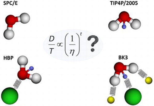
GRAPHICAL ABSTRACT

KEYWORDS:

• Water
• self-diffusivity
• shear viscosity
• molecular dynamics
• Stokes–Einstein relation

1. Introduction and background

There could be no life, as we know it, on planet Earth without the presence of water since according to Kumar [1] ‘ … water is probably the most important liquid for life’. Therefore, the importance of water cannot be overemphasised. While water is among the smallest molecules that can be encountered in nature, it exhibits extremely complex behaviour and a large number of counterintuitive anomalies in its physical properties (Gallo et al. [2]). Over the years, numerous studies have focused on examining various aspects related to different water properties [2]. To this purpose, experimental measurements, atomistic scale simulations, and continuum-scale theories have been employed in order to explain the ‘often-unexpected’ behaviour exhibited by the thermodynamic, transport or structural properties of the various water isomorphs [2].

Properties of interest to the current study are the translational self-diffusion coefficient and the shear viscosity of water. Both dynamic properties exhibit anomalous behaviour; namely a non-monotonic dependence on pressure [3]. In particular, the self-diffusion coefficient of water reaches a maximum as a function of pressure. This is experimentally observable in supercooled water for both the translational [4,5] and rotational [6,7] motion of water. Additional experimental measurements for the translational self-diffusion coefficient of water have been reported, among others, by Krynicki et al. [8], and Price et al. [9]. The water shear viscosity reaches a minimum as a function of pressure. Recent experiments by Singh et al. [10] have located the minimum at 244 K and 200 MPa where a 42% reduction was reported in the shear viscosity, compared to the value at ambient pressure. Experimental measurements for the shear viscosity of water have also been reported by Dehaoui et al. [11] and in references therein. It should be noted, however, that experimental measurements for the shear viscosity of water are relatively scarce, particularly at supercooled conditions.

Experimental measurements are essential for model development and validation. However, due to their cost and time requirements, significant effort is devoted to minimise the amount of experimental measurements required, while at the same time computational or theoretical methods can fill in the missing gap. An additional complication that can be encountered during experimental studies on metastable water is the homogeneous ice nucleation in supercooled water or of a vapour phase in stretched water. The ice or vapour phase nucleation occurs due to the long time required for the experimental measurements [2]. An attractive alternative to avoid this problem is molecular dynamics (MD) simulations. In MD, short time scales, i.e. in the order of nanoseconds, are considered, from which structural, thermodynamic and transport properties of water can be computed [12]. The accuracy of these computations strongly depends on the description of the intra- and intermolecular interactions of water molecules, the so-called force field.

During the development of water force fields, the self-diffusion coefficient is very often considered to test the performance [13] of the new models. This is usually done at ambient conditions, i.e. 1 bar and 298 K. Therefore, numerous MD values for the water self-diffusion coefficient are available in the literature for ambient conditions. A collection of these data along with a detailed discussion on the performance of various water force fields for predicting the self-diffusivity can be found in the recent review by Tsimpanogiannis et al. [14]. While a plethora of values is available (see for example the extended lists that are presented in ref [14]), a significant amount of data are of either limited or questionable value, since the water self-diffusivities were reported without taking into account the required corrections for the system size effects (SSE) which can be achieved following the Yeh and Hummer [15] approach. For example, extensive simulations in the temperature range 210–350 K have been reported by Starr et al. [16] using 216 SPC/E [17] water molecules, Agarwal et al. [18] used 256 SPC/E [17], TIP4P [19], TIP4P/2005 [20] and TIP5P [21] water molecules, while Kumar et al. [22] used 512 TIP5P [21] water molecules. In all these cases, the correction that should be applied to the reported self-diffusivity values is often in the range of 5–20% [14,23,24]. As discussed in Tsimpanogiannis et al. [14], it is important that the self-diffusion coefficient values are either corrected to account for SSE (e.g. using the Yeh and Hummer [15] approach) or big systems (>1,000 water molecules) should be used in the MD simulations. Such systems have been identified to be adequately large and the calculated self-diffusivities are close to those of an infinite system [14]. In the current study, we use self-diffusion coefficients of water computed from MD simulations that are either:

1. Reported to be corrected through the Yeh and Hummer [15] approach. Such are the cases of Jiang et al. [25] who considered the BK3 [26] and HBP [25] water models, Guillaud et al. [27] that examined the TIP4P/2005f [28] water model, de Hijes et al. [29] that used the TIP4P/2005 [20] water model, or

2. are obtained from MD simulations of more than 1,000 water molecules. Such are the cases reported by Guevara-Carrion et al. [30] for 2,048 SPC [31], SPC/E [17], TIP4P [19], or TIP4P/2005 [20] water molecules, Moultos et al. [32] for 2,000 SPC/E or TIP4P/2005 water molecules, Shvab and Sadus [33] for 1,728 TIP4P/2005 or TIP4P/2005f water molecules, Park et al. [34] for 1,024 SPC/E water molecules, Koster et al. [35] for 3,000 TIP4P/2005, TIP4P-TPSS [36], TIP4P-TPSS-D3 [36], and Huang et al. [37] (TIP4P-type), water molecules, and Kawasaki and Kim [38] for 1,000 TIP4P/2005 water molecules.

These studies (shown also in Table 1) reported also values for the water shear viscosity at the same state points. It should be noted that Moultos et al. [32] did not report water shear viscosity data. For the particular state points, the MD simulations of Michalis et al. [39] have been used in the analysis presented in the current study. Additional MD studies that satisfy either one of the aforementioned two criteria for SSE corrections for the self-diffusion coefficients are also available (e.g. Kiss and Baranyai [40] reported corrected values that accounted for SSE for the BK3 water model, Kumar et al. [22] and Becker et al. [41] used 1,718 ST2 [42] water molecules in their studies, while a more detailed list of references can be found in [14]). However, these studies are not considered any further in the current study, since due to reasons of self-consistency (to be discussed subsequently) it is essential to have also available shear viscosities computed from MD simulations at the same state points. It is important to note that due to the more demanding nature of the calculation that is required for the shear viscosity of water (especially at low temperatures [38]); MD simulations are less readily available. In addition to the references that are shown in Table 1, shear viscosity studies for various water force fields have also been reported by Fuhrmans et al. [43], Raabe and Sadus [44], Fuentes-Azcatl and Alejandre [45], Fuentes-Azcatl et al. [46], Ding et al. [47], and Köster et al. [48].

Table 1. List of studies for which MD-calculated values for self-diffusivities and shear viscosities are available, along with the corresponding exponents for the fractional Stokes-Einstein relation that are calculated in the current study.

			Intercept	slope (s)	Intercept	slope (t)
Authors	Water Model	T range [K]	(D vs. T/n)	(D vs. T/n)	(D/T vs. n)	(D/T vs. n)
Dehaoui et al. [11]	Experimental	238–273	−30.355	0.812	−31.328	−0.800
Dehaoui et al. [11]	Experimental	274–373	−31.968	0.950	−32.192	−0.941
Harris [49]	Experimental	238–273	N/A	N/A	−5.297	−0.668
Harris [49]	Experimental	274–623	N/A	N/A	−4.977	−0.943
This work (SSE ^(*) included)	SPC/E	220–270	−31.949	0.946	−32.223	−0.941
This work (SSE included)	SPC/E	280–560	−31.877	0.942	−32.071	−0.924
This work (SSE included)	TIP4P/2005	220–270	−30.921	0.855	−31.689	−0.848
This work (SSE included)	TIP4P/2005	280–310	−31.119	0.883	−31.628	−0.861
This work ^(**) (SSE included)	TIP4P/2005	280–623	−31.793	0.934	−32.017	−0.913
Guevara-Carrion et al. [30]	SPC/E	280–373.15	−31.194	0.898	−31.597	−0.873
Moultos et al. [32]	SPC/E	298.15–623.15	−31.872	0.945	−32.044	−0.925
Park et al. [34]	SPC/E	243–273	−30.135	0.819	−31.038	−0.801
Park et al. [34]	SPC/E	273–550	−31.873	0.941	−32.064	−0.921
Guevara-Carrion et al. [30]	TIP4P/2005	273.15–400.15	−30.804	0.862	−31.373	−0.831
Moultos et al. [32]	TIP4P/2005	298.15–623.15	−32.439	0.977	−32.509	−0.968
Shvab & Sadus [33]	TIP4P/2005	670	−8.9073	0.798	−10.223	−0.798
Jiang et al. [25]	TIP4P/2005	298.15–523.15	−10.8148	0.918	−11.0311	−0.885
Koster et al. [35]	TIP4P/2005	280–340	−11.115	0.944	−11.356	−0.932
Kawasaki & Kim [38]	TIP4P/2005	190–260	−32.706	1.029	−32.542	−1.027
Kawasaki & Kim [38]	TIP4P/2005	260–300	−30.963	0.811	−32.032	−0.820
de Hijes et al. [29]	TIP4P/2005	200–270	−30.443	0.814	−31.428	−0.807
de Hijes et al. [29]	TIP4P/2005	280–300	−31.623	0.923	−32.011	−0.915
Shvab & Sadus [33]	TIP4P/2005f	670	−9.8614	0.859	−10.782	−0.859
Guillaud et al. [27]	TIP4P/2005f	225–273	−10.178	0.859	−10.916	−0.851
Guillaud et al. [27]	TIP4P/2005f	273–360	−11.245	0.950	−11.462	−0.941
Koster et al. [35]	Huang et al.	280–340	−6.008	0.553	−8.005	−0.480
Koster et al. [35]	TIP4P-TPSS	280–340	−13.433	1.110	−12.972	−1.132
Koster et al. [35]	TIP4P-TPSS-D3	280–340	−9.583	0.826	−10.319	−0.792
Jiang et al. [25]	HBP	298.15–523.15	−31.618	0.920	−31.898	−0.896
Jiang et al. [25]	BK3	298.15–523.15	−32.173	0.957	−32.335	−0.945

^(*) SSE: System Size Effects

^(**) MD data in the range 220–310 K are from the current work, while for higher temperatures the MD data are from Moultos et al. [32].

The classical hydrodynamic theory of Stokes–Einstein (SE) provides a link between the intra-diffusion coefficient D (also applicable to the self-diffusion coefficient) of a particle and its radius r in a continuum with shear viscosity, $\eta$. The fractional Stokes–Einstein (FSE) relation has been found to correlate adequately both model and real fluids. According to Harris [49], there are two forms of the FSE that are encountered in the literature and provide the temperature dependence of the two transport properties, D and $\eta$, that are of interest to the current study: (1) $\begin{array}{rl}\frac{D}{T}& \propto {\left(\frac{1}{\eta }\right)}^t\end{array}$(1) (2) $\begin{array}{rl}D& \propto {\left(\frac{T}{\eta }\right)}^s\end{array}$(2) where the exponents t, s can be determined from the slopes of log–log plots. When t or s are equal to 1, the SE relation is valid and therefore, preserved. For all other cases, the SE relation is violated, while the FSE is valid (i.e. the exponent is less than one). Based on available experimental measurements, for the case of water, Harris [49] reported the following values for the exponent t: −0.9429 for $623\ge T/K\ge 274$, and −0.6684 for $273\ge T/K\ge 238$.

To test directly if the SE relation is violated or preserved by a set of data (which can be either experimental or MD-based), the method requires self-consistency during the calculation. Namely, both the shear viscosity and the self-diffusivity should be either measured experimentally, or both should be calculated from MD simulations using the same water model and the same number of molecules. Essentially, the mixing of experimental values with MD-obtained values or the mixing of values from different water models can result in the destruction of the self-consistency of the calculation. This should be avoided in all cases. To overcome the lack of MD-calculated shear viscosity data, discussed earlier, the structural relaxation time, $\tau$, has often been used as a proxy to the shear viscosity. This results from the Gaussian solution to the diffusion equation which is given by $F_s(k,t)=\exp (-k^{2}Dt)\equiv \exp (-t/\tau )$, where $F_s(k,t)$ is the self-intermediate scattering function and k is the associated wave vector[50].

Namely, for this case an indirect test is performed. A number of highly cited studies have followed that route including those by Becker et al. [41], Kumar et al. [22], Mazza et al. [51], Xu et al. [52], and Stanley et al. [53]. Such studies are based on the simple approximation of proportionality between shear viscosity and relaxation time (i.e. $\tau \sim \eta$) that is often invoked. The particular approximation is further based on the assumed constancy of the instantaneous shear modulus, $G_{\mathrm{\infty }}$. Based on extensive MD simulations that were reported by Shi et al. [50], it was concluded that for both model atomic and molecular systems a temperature dependence exists for $\tau /\eta$. Therefore, it is not advisable to use the relaxation time as a proxy for the shear viscosity when examining the validity of the SE relation for a system. This observation was also confirmed for the case of the TIP4P/2005f water model by Guillaud et al. [27]. Kawasaki and Kim [38] offered a similar analysis based on the TIP4P/2005 water model. Finally, a similar discussion is also presented in the experimental study of Dehaoui et al. [11].

A number of the previously mentioned studies that used the relaxation time as a proxy to the shear viscosity focused at the supercooled conditions and reported the violation of the SE relation. Therefore, it is essential to revisit such issues, taking into further consideration the important conclusions that were discussed by Shi et al. [50] and Guillaud et al. [27]. The objectives of the current study are:

1. To report an extensive and consistent set of MD simulations for the self-diffusivity and shear viscosity of water in the temperature range 200–623 K and pressures 1 and 1000 bar. Two of the most commonly used water models are considered, namely, the SPC/E [17] and TIP4P/2005 [20].

2. To re-evaluate the validity or violation of the SE relation for these two water models, taking into account the following two important issues: First, that the values of the self-diffusivities are corrected in order to account for SSE, and second, that the shear viscosity is used in the analysis, instead of the often-used relaxation time. The calculated fractional exponents are compared against those obtained from the analysis of the experimental data and the TIP4P/2005 is found to outperform SPC/E.

3. To perform a similar analysis for the validity or violation of the SE relation for all other water models, for which MD-calculated values for self-diffusivities (corrected for SSE) and shear viscosities are available, including SPC/E, TIP4P/2005, TIP4P/2005f, HBP, and BK3.

4. To further discuss the issue of the discrepancy at supercooled conditions, between the exponents for the FSE relation, t, reported by Dehaoui et al. [11], and Harris et al. [49].

The paper is organised as follows: First, we briefly present the computational methodology that was followed. Second, we discuss the main results obtained in the current study. We end with the conclusions and some future outlook.

2. Simulation details

MD simulations have been carried out to compute the self-diffusivity and shear viscosity of water at temperatures in the range of 220–560 K, and at two pressures, 1 and 1,000 bar. For all transport coefficient computations, the OCTP plugin [54] in the LAMMPS [55] software package (version released on November 27, 2018) was used. The OCTP plugin uses the Einstein relations along with the order-n algorithm ([12], [56]) to compute ‘on-the-fly’ transport coefficients in LAMMPS. For all relevant details on the inner workings of the OCTP plugin and the self-diffusivity and viscosity computations the reader can refer to the original work by Jamali et al. [54]. All reported self-diffusivities that are calculated in the current study are corrected for system size effects using the Yeh and Hummer correction ([57,15]). For the particular new simulations the density is high, therefore, water behaves like a liquid. As discussed in Jamali et al. [24] for such cases the Yeh-Hummer correction works well. For additional elaborate discussions on the effect of system size on the computation of self-diffusivity the reader is referred to the original works by Dünweg and Kremer [57], Yeh and Hummer [15], to recent literature ([24,58,59]), as well as at the recent review by Tsimpanogiannis et al. [14]. On the other hand, the shear viscosity does not suffer for system size effects [15,58,24].

All MD simulations were performed in a cubic simulation box with periodic boundary conditions imposed in all directions. For the representation of water, the SPC/E [17] and TIP4P/2005 [19] force fields were used, along with the Lorentz-Berthelot combining rules [60] for interactions of unlike atoms. The SHAKE algorithm in LAMMPS was used to fix the O – H and H – H distances of the water molecules fixed, according to the original rigid force fields. The electrostatics interactions were handled with the particle-particle, particle-mesh (PPPM) method in LAMMPS [55]. The cut-off radius for both van der Waals (Lennard-Jones) and electrostatic interactions was set to 10 Å. Analytic tail corrections were applied to the energy and pressure. 500 water molecules were used in all simulations.

The simulation scheme followed in this study is described in detail in the Supporting Information of our earlier work [54]. In short, initial configurations for the MD simulations were created using ‘PACKMOL’ [61]. Then energy minimisation and a short equilibration run was performed in the NPT ensemble. Subsequently, a longer NPT run was performed, from which the average box size length, corresponding to the correct density of the system, was obtained. Finally, this average box size was used for the production runs in the NVT ensemble. For the computation of self-diffusivities and viscosities, and their respective uncertainties, 5 independent runs of 10 ns were performed, each one starting from a different initial configuration. All the MD-calculated values for densities, self-diffusivities and shear viscosities, along with their uncertainties, are reported in Tables S1 and S2 of the Supplemental Information for the cases of SPC/E and TIP4P/2005 respectively.

3. Results and discussion

To validate our MD simulation results, we initially performed a series of comparisons with available experimental data, focusing primarily on densities, self-diffusivities and shear viscosities. The MD-calculated liquid densities, plotted as a function of temperature for 1 and 1,000 bar, are shown in Figure 1a. The MD values are compared with experimental values. For temperatures higher than 274 K, the values reported from NIST [62] are used, while for values lower than 274 K, the experimental measurements reported in [63] are used. As we can observe in Figure 1a, the performance of TIP4P/2005 is superior to that of SPC/E, regarding its ability to accurately capture the liquid density. For temperatures higher than approx. 310 K, both water models yield almost identical liquid densities. At lower temperatures, SPC/E over-predicts the liquid density. This effect is stronger at the lower pressures. The TIP4P/2005 reproduces accurately the water density maximum, while it follows closely the density decrease that occurs at the lower temperatures. Our calculations with the TIP4P/2005 are in very good agreement with those reported by Abascal and Vega [64] in which 500 water molecules were used. This is clearly shown in Figure 1b. Additional discussion regarding the behaviour at very low T’s can be found in the paper by Abascal and Vega [64].

Figure 1. (a) Density plotted as a function of temperature for SPC/E (denoted with triangles) and TIP4P/2005 (denoted with circles) water models. Blue colour denotes values at 1 bar, while red colour at 1,000 bar. Solid lines (for T > 273 K) denote values from NIST [62] while dashed lines (for T < 273 K) experimental values reported in [63]. The dashed-dotted vertical black line indicates the temperature equal to 273.15 K. The inset of the lower-left side is a blow-up of the temperature range 180–380 K. (b) Comparison of densities for TIP4P/2005 calculated in the current study (denoted with circles) and in the work of Abascal and Vega [64] (denoted with crosses).

Figure 2 provides a similar comparison of the MD values obtained in the current study, with available experimental measurements for the case of shear viscosity (Figure 2a) and self-diffusivity corrected for SSE (Figure 2b) of the two water models considered. Both figures are shown as Arrhenius plots (i.e. the property is plotted as a function of the inverse temperature). We observe that for both properties, $\eta$ and D, the performance of the TIP4P/2005 is significantly better, especially at the lower temperatures, where the deviation from ‘Arrhenius-type’ behaviour becomes stronger. For temperatures higher than approx. 280 K, both water models give very similar results following closely the Arrhenius behaviour. Additional discussion that is pertinent to the issue can be found in the review of Tsimpanogiannis et al. [14]. The poor quality for the prediction of the shear viscosity and self-diffusivity by SPC/E at supercooled conditions is directly associated with the poor quality of the corresponding density predictions at the same temperature range [32,65,66].

Figure 2. Arrhenius plots for: (a) the water shear viscosities, and (b) the water self-diffusion coefficients. MD results from SPC/E water model are denoted with triangles and circles, while MD results from TIP4P/2005 are denoted with crosses and x’s. Blue colour in symbols or lines denotes values at 1 bar, while red colour at 1,000 bar. The dashed-dotted vertical black line indicates temperatures equal to 273.15 K. Uncertainties are reported in the Supplemental Information. In the water shear viscosity plot (a) solid lines denote values from NIST [62], while the dashed black line denotes the experimental measurements by Dehaoui et al. [11]. In the water self-diffusion coefficient plot (b) the dashed lines denote experimental measurements from: Price et al. [9] (1 bar, T < 273 K), Krynicki et al. [8] (1 bar, T > 273 K), Prielmeir et al. [4] (1,000 bar, T < 273 K) and Krynicki et al. [8] (1,000 bar, T > 273 K).

Figure 3 shows a plot of the self-diffusion coefficient of water as a function of the inverse temperature at the two pressures, 1 and 1,000 bar, under examination. Figure 3a shows the MD results for the case of the SPC/E water model, while Figure 3b shows the corresponding results for the case of TIP4P/2005. The new MD data that were calculated in the current study for both water models have been correlated using four different types of equations. Namely, an Arrhenius (ARH) law [67] given by: (3) $\begin{array}{r}{D}_{ARH}=D_{0}exp\left(-\frac{\alpha }{T}\right)\end{array}$(3) a Vogel – Fulcher – Tamann (VFT) equation [68]: (4) $\begin{array}{r}{D}_{VFT}=exp\left[\frac{-\alpha }{(T-\beta )}-\gamma \right]\end{array}$(4) a Speedy – Angel (SA) power law [69] described by the following equation: (5) $\begin{array}{r}{D}_{SA}=D_o{\left(\frac{T}{215.05}-1\right)}^{\gamma }\end{array}$(5) and a Mode-Coupling Theory [70] (MCT) type of equation given by: (6) $\begin{array}{r}{D}_{MCT}=D_o(T-220{)}^{-\gamma }\end{array}$(6) where $D_o,\alpha ,\beta ,\gamma$are fit parameters given in Table 2. For the case of the Arrhenius law, $\alpha =\frac{E_a}{R}$, where R is the universal gas constant and E_a is the Arrhenius activation energy (in kJ/mol). In Table 2, the values for the percentage average absolute deviation (% AAD), defined as $\mathrm{\%}AAD=100\times \left|\frac{D_{}^{calc}-D_{}^{exp}}{D_{}^{exp}}\right|$ are also shown. The superscripts calc and exp denote the calculated and experimental values of the self-diffusion coefficient of water, respectively. It should be noted that for the reported values of Table 2, the entire temperature range of data has been used for the fitting. We observe that for temperatures higher than approx. 320 K, the calculations from all four equations essentially collapse on top of the MD values. However, for the case of the lower temperatures, the MD data are described more accurately by the SA-type equation, followed by the MCT-type equation.

Figure 3. Self-diffusion coefficients of water as a function of the inverse temperature at 1 bar (blue circles) and 1,000 bar (red triangles) for two water models: (a) SPC/E, and (b) TIP4P/2005. Black diamonds denote the MD results of Moultos et al. [32] for T > 273 K. The dashed lines correspond to correlations of all the MD data of the current study. Colour code of dashed lines. Arrhenius (ARH) law: green line; Vogel–Fulcher–Tamann (VFT) equation: magenta line; Speedy – Angel (SA) power law: cyan line, and Mode Coupling Theory (MCT): black line. The dashed-dotted vertical black line indicates temperatures equal to 273.15 K. Uncertainties are reported in the Supplemental Information.

Table 2. Parameters for the MD self-diffusion coefficient of water calculated using different correlations and % average absolute deviation (% AAD) between experimental data and correlations. The MD data are corrected to account for system size effects.

Correlation	Do (m^2/s)	α (K)	β (K)	γ (−)	% AAD
SPC/E water model (220–560 K)
ARH-type	$0.4625\times {10}^{-6}$	$1.510\times {10}^3$	na	na	30.64
VFT-type	na	$1.2308\times {10}^3$	39.7380	14.9288	18.86
SA-type	$1.399\times {10}^{-8}$	na	na	1.6881	9.55
MCT-type	$2.1508\times {10}^{-12}$	na	na	1.6426	13.77
TIP4P/2005 water model (220–623 K)
ARH-type	$0.6218\times {10}^{-6}$	$1.681\times {10}^3$	na	na	49.14
VFT-type	na	$2.043\times {10}^3$	−48.3683	13.9386	13.94
SA-type	$1.2673\times {10}^{-8}$	na	na	1.8713	9.86
MCT-type	$0.7026\times {10}^{-12}$	na	na	1.8332	14.86

na: not applicable

The validity or violation of the SE relation is tested for a number of cases from the literature, in addition to the MD results obtained from the current study. To this purpose, both exponents t, and s appearing in Equations (1) and (2) are determined from the slopes of the appropriate log–log plots and the obtained results are reported in Table 1. Small variations are observed between the values of the exponents t, s. Nevertheless, the general conclusion regarding the violation of the SE relation remains unchanged. Starting with the experimental data, we observe that for temperatures higher than 274 K, both the experimental data used by Harris [49] and those reported by Dehaoui et al. [11] result in a value for the exponent t equal to −0.943 and −0.941 respectively, which are in very good agreement and differ between each other only by 0.16%. On the other hand, for temperatures lower than 274 K, the corresponding values are −0.668 and −0.800 respectively. Dehaoui et al. attributed this difference to the use of erroneous experimental data for viscosities by Harris. Therefore, a violation of the SE relation is observed for the experimental data, having different slopes for temperatures above or below 274 K.

As a next step, the new MD data calculated in the current study are analysed. We find that for temperatures higher than 274 K, values for the exponent t, equal to −0.924 and −0.913, are calculated for the case of SPC/E and TIP4P/2005 water models respectively. These values correspond to a 1.8% or 3.0% absolute deviation for the SPC/E and TIP4P/2005 respectively, from the value calculated from the experimental data of Dehaoui et al. [11]. For temperatures lower than 274 K, the corresponding values for SPC/E and TIP4P/2005 are −0.941 and −0.848. Similarly, these values correspond to a 17.7% or 6.0% absolute deviation for the SPC/E and TIP4P/2005 respectively, from the value calculated from the experimental data of Dehaoui et al. [11]. We notice that the inaccuracies of the SPC/E model in the prediction of the viscosities and the self-diffusivities that were observed at Figure 2, are also reflected in the calculation of the exponent t (or similarly s). It is evident from the MD results of the current study that a violation of the SE relation is observed. The obtained exponents have different values for temperatures above or below 274 K.

It should be noted that the exponents for t that are obtained from the current study for the case of TIP4P/2005 (both below and above 274 K) are in excellent agreement with those reported by de Hijes et al. [29], who also used TIP4P/2005. Both studies are also in good agreement with the experimental fractional exponents. Note also that the calculated fractional exponents for the case of the TIP4P/2005f MD simulations reported by Guillaud et al. [27] are in excellent agreement with the values calculated from the experimental data reported by Dehaoui et al. [11]. The poor agreement of the calculated fractional exponents for the cases of TIP4P-TPSS, TIP4P-TPSS-D3 and Huang et al. water models (MD data reported by Koster et al. [35]) is a result of their poor performance in predicting accurately the densities, as well as the self-diffusivities and shear viscosities of water. An overall picture of all the exponents t that were calculated during the analysis performed in the current study is shown in Figure 4. In particular, Figure 4a shows the results for temperatures below 274, while Figure 4b for temperatures above 274 K. Furthermore, for the case of temperatures that are lower than 274 K, all the MD data that were analysed in the current study are in support of the exponent that was reported by Dehaoui et al. [11]. The particular case is a good example when MD simulations can contribute in resolving possible discrepancies in the experimental measurements.

Figure 4. Comparison of the various calculated fractional exponents, t, with the experimental value for two cases: (a) temperatures below 274 K and (b) temperatures above 274 K. Data sources are the same as in Table 1. The vertical dashed red lines indicate the corresponding values obtained from the experimental data reported by Dehaoui et al. [11].

An additional pictorial representation of the results that are shown in Table 1 can be found in Figures 5–7. Figure 5 shows the testing of the Stokes–Einstein relation given by Equation (2): $D\sim (T/\eta )$ for the SPC/E, while Figure 6 shows the corresponding case for the TIP4P/2005 water model. In both cases Figures (5a) or (6a) show the results of the current study, while Figures (5b) or (6b) show the corresponding cases from other available studies in the literature. Similarly, Figure 7 shows the corresponding cases that were reported by Jiang et al. [25] for the polarisable models BK3 and HBP. It should be noted here that only a limited number of state points have been reported, all of which are above 298 K. The presence of additional state points would be desirable for a more accurate calculation of the exponent of the FSE relation for the two polarisable models. Furthermore, the corresponding behaviour at supercooled conditions is still missing.

Figure 5. Testing of the Stokes-Einstein relation $D\sim (T/\eta )$ for the SPC/E water model: (a) This work, and (b) Other studies. The symbols denote MD results and the dashed lines are from experimental data (Dehaoui et al. [11]) fitted by the fractional Stokes-Einstein relation $D\sim (T/\eta {)}^s$. The dashed-dotted black line indicates the experimental data slope for T > 273.15 K. The dashed black line indicates the experimental data slope for T < 273.15 K. The vertical black dotted line indicates temperatures equal to 273.15 K.

Figure 6. Testing of the Stokes-Einstein relation $D\sim (T/\eta )$ for the TIP4P/2005 water model: (a) This work, and (b) Other studies. The symbols denote MD results and the dashed lines are from experimental data (Dehaoui et al. [11]) fitted by the fractional Stokes-Einstein relation $D\sim (T/\eta {)}^s$. The dashed-dotted black line indicates the experimental data slope for T > 273.15 K. The dashed black line indicates the experimental data slope for T < 273.15 K. The vertical black dotted line indicates temperatures equal to 273.15 K.

Figure 7. Testing of the Stokes-Einstein relation $D\sim (T/\eta )$ for various water models. The symbols denote published MD results and the dashed lines are from experimental data (Dehaoui et al. [11]) fitted by the fractional Stokes-Einstein relation $D\sim (T/\eta {)}^s$.

4. Conclusions

The current study focused primarily on the translational self-diffusion coefficient and the shear viscosity of the SPC/E and TIP4P/2005 water models in the temperature range 220–560 K and 1 or 1,000 bar. We reported extensive novel MD simulation results that were used, subsequently, to calculate the fractional exponents of the FSE relation. The simulations with both water models concluded that the SE is violated for the entire temperature range that was considered. Different exponents were obtained for temperatures above or below 274 K. While both water models exhibit comparable behaviour for temperatures higher than 274 K, the TIP4P/2005 has significantly superior behaviour at supercooled conditions. This is a direct consequence of its better performance in the prediction of densities, self-diffusivities and shear viscosities.

The accurate knowledge of the exponents in the FSE relation is a valuable tool since estimates for the shear viscosities can be obtained, once values for the self-diffusivities are readily available (either from MD simulations or experimental measurements). It should be noted that obtaining estimates for shear viscosities requires a significantly more tedious effort than self-diffusivities.

It is evident from the discussion presented here that there are two major requirements in order to perform the analysis of the validity or violation of the SE relation: (i) the self-diffusivities should be either corrected for SSE or be obtained from systems with more than 1,000 water molecules, and (ii) the shear viscosity should be used instead of the relaxation time that is often used as a proxy. Consequently, only a handful of studies are found that satisfy both the aforementioned requirements. In that respect, the TIP4P/2005 is the more widely studied water model, followed by SPC/E and TIP4P/2005f, having MD data both above and below 274 K. The cases of HBP and BK3 are only limited to temperatures above 298 K. Therefore, there is ample space to perform simulations in order to examine the behaviour of HBP and BK3 regarding the validity of violation of the SE relation, especially at supercooled conditions. Furthermore, no other polarisable water model has been examined regarding this particular issue in any kind of conditions.

Statement of significance

In this study, we present an extensive and consistent set of molecular dynamics simulations for the self-diffusivity and shear viscosity of water for a wide temperature and pressures range for SPC/E and TIP4P/2005 water models. We evaluate the validity of the Stokes–Einstein (SE) relation for these two water models, considering that the self-diffusivities are corrected for system size effects, and that the shear viscosities are used, instead of the often-used relaxation time. We perform a similar analysis for the validity of the SE relation for all other water models, for which MD-calculated values for self-diffusivities and shear viscosities are available.

Acknowledgments

This work was sponsored by NWO Exacte Wetenschappen (Physical Sciences) for the use of supercomputer facilities, with financial support from the Nederlandse Organisatie voor Wetenschappelijk Onderzoek (Netherlands Organisation for Scientific Research, NWO). T.J.H.V. acknowledges NWO-CW (Chemical Sciences) for a VICI grant. Othonas A. Moultos gratefully acknowledges the support of NVIDIA Corporation with the donation of the Titan V GPU used for this research. We are grateful to Prof. L. Jolly for providing us with the Table of the calculated values for self-diffusivities and viscosities for the TIP4P/2005f water model that was reported in ref [27].

Disclosure statement

No potential conflict of interest was reported by the authors.

Additional information

Funding

This work was supported by Nederlandse Organisatie voor Wetenschappelijk Onderzoek: [Grant Number NWO-CW,NWO-PW].

References

- P. Kumar, Proc. Natl. Acad. Sci. USA. 103, 12955 (2006). doi: 10.1073/pnas.0605880103
- P. Gallo, K. Amann-Winkel, C.A. Angell, M.A. Anisimov, F. Caupin, C. Chakravarty, E. Lascaris, T. Loerting, A.Z. Panagiotopoulos, J. Russo, J.A. Sellberg, H.E. Stanley, H. Tanaka, C. Vega, L. Xu and L.G.M. Pettersson, Chem. Rev. 116, 7463 (2016). doi: 10.1021/acs.chemrev.5b00750
- Y. Xu, N.G. Petrik, R.S. Smith, B.D. Kay and G.A. Kimmel, Proc. Natl. Acad. Sci. USA. 113, 14921 (2016). doi: 10.1073/pnas.1611395114
- F.X. Prielmeir, E.W. Lang, R.J. Speedy and H.-D. Ludemann, Ber. Bunsengesell. Phys. Chem. 92, 1111 (1988). doi: 10.1002/bbpc.198800282
- K.R. Harris and P.J. Newitt, J. Chem. Eng. Data. 42, 346 (1997). doi: 10.1021/je9602935
- E.W. Lang and H.D. Ludemann, Ber. Bunsengesell. Phys. Chem. 85, 603 (1981). doi: 10.1002/bbpc.19810850716
- M.R. Arnold and H.-D. Ludemann, Phys. Chem. Chem. Phys. 4, 1581 (2002). doi: 10.1039/b110639m
- K. Krynicki, C.D. Green and D.W. Sawyer, Faraday Discuss. Chem. Soc. 66, 199 (1978). doi: 10.1039/dc9786600199
- W.S. Price, H. Ide and Y. Arata, J. Phys. Chem. A. 103, 448 (1999). doi: 10.1021/jp9839044
- L.P. Singh, B. Issenmann and F. Caupin, Proc. Natl. Acad. Sci. USA. 114, 4312 (2017). doi: 10.1073/pnas.1619501114
- A. Dehaoui, B. Issenmann and F. Caupin, Proc. Natl. Acad. Sci. USA. 112, 12020 (2015). doi: 10.1073/pnas.1508996112
- D. Frenkel and B. Smit, Understanding Molecular Simulation: From Algorithms to Applications, 2nd ed. (Academic Press, San Diego, CA, 2002).
- C. Vega and J.L.F. Abascal, Phys. Chem. Chem. Phys. 13, 19663 (2011). doi: 10.1039/c1cp22168j
- I.N. Tsimpanogiannis, O.A. Moultos, L.F.M. Franco, M.B.d.M. Spera, M. Erdos and I.G. Economou, Mol. Simul. 45, 425 (2019). doi: 10.1080/08927022.2018.1511903
- I.C. Yeh and G. Hummer, J. Phys. Chem. B. 108, 15873 (2004). doi: 10.1021/jp0477147
- F.W. Starr, F. Sciortino and H.E. Stanley, Phys. Rev. E. 60, 6757 (1999). doi: 10.1103/PhysRevE.60.6757
- H.J.C. Berendsen, J.R. Grigera and T.P. Straatsma, J. Phys. Chem. 91, 6269 (1987). doi: 10.1021/j100308a038
- M. Agarwal, M.P. Alam and C. Chakravarty, J. Phys. Chem. B. 115, 6935 (2011). doi: 10.1021/jp110695t
- W.L. Jorgensen, J. Chandrasekhar, J.D. Madura, R.W. Impey and M.L. Klein, J. Chem. Phys. 79, 926 (1983). doi: 10.1063/1.445869
- J.L.F. Abascal and C. Vega, J. Chem. Phys. 123, 234505 (2005). doi: 10.1063/1.2121687
- M.W. Mahoney and W.L. Jorgensen, J. Chem. Phys. 112, 8910 (2000). doi: 10.1063/1.481505
- P. Kumar, S.V. Buldyrev, S.R. Becker, P.H. Poole, F.W. Starr and H.E. Stanley, Proc. Natl. Acad. Sci. USA. 104, 9575 (2007). doi: 10.1073/pnas.0702608104
- S. Tazi, A. Boan, M. Salanne, V. Marry, P. Turq and B. Rotenberg, J. Phys. Condens. Matter. 24, 284117 (2012). doi: 10.1088/0953-8984/24/28/284117
- S.H. Jamali, R. Hartkamp, C. Bardas, J. Söhl, T.J.H. Vlugt and O.A. Moultos, J. Chem. Theory Comput. 14, 5959 (2018). doi: 10.1021/acs.jctc.8b00625
- H. Jiang, O.A. Moultos, I.G. Economou and A.Z. Panagiotopoulos, J. Phys. Chem. B. 120, 12358 (2016). doi: 10.1021/acs.jpcb.6b08205
- P.T. Kiss and A. Baranyai, J. Chem. Phys. 138, 204507 (2013). doi: 10.1063/1.4807600
- E. Guillaud, S. Merabia, D. de Ligny and L. Joly, Phys. Chem. Chem. Phys. 19, 2124 (2017). doi: 10.1039/C6CP07863J
- M.A. González and J.L.F. Abascal, J. Chem. Phys. 135, 224516 (2011). doi: 10.1063/1.3663219
- P.M. de Hijes, E. Sanz, L. Joly, C. Valeriani and F. Caupin, J. Chem. Phys. 149, 094503 (2018). doi: 10.1063/1.5042209
- G. Guevara-Carrion, J. Vrabec and H. Hasse, J. Chem. Phys. 134, 074508 (2011). doi: 10.1063/1.3515262
- H.J.C. Berendsen, J.P.M. Postma, W.F. van Gunsteren and J. Hermans, in Intermolecular Forces, edited by B. Pullman (Dordrecht: D. Reidel Publishing Company, 1981). pp. 331–342.
- O.A. Moultos, I.N. Tsimpanogiannis, A.Z. Panagiotopoulos and I.G. Economou, J. Phys. Chem. B. 118, 5532 (2014). doi: 10.1021/jp502380r
- I. Shvab and R.J. Sadus, Phys. Rev. E. 92, 012124 (2015). doi: 10.1103/PhysRevE.92.012124
- D.K. Park, B.-W. Yoon and S.H. Lee, Bull. Korean Chem. Soc. 36, 492 (2015).
- A. Köster, T. Spura, G. Rutkai, G. Rutkai, J. Kessler, H. Wiebeler, J. Varbec and T.D. Kuhne, J. Comput. Chem. 37, 1828 (2016). doi: 10.1002/jcc.24398
- T. Spura, C. John, S. Habershon and T.D. Kuhne, Mol. Phys. 113, 808 (2015). doi: 10.1080/00268976.2014.981231
- Y.-L. Huang, T. Merker, M. Heilig, H. Hasse and J. Vrabec, Ind. Eng. Chem. Res. 51, 7428 (2012). doi: 10.1021/ie300248z
- T. Kawasaki and K. Kim, Sci. Adv. 3, e1700399 (2017). doi: 10.1126/sciadv.1700399
- V.K. Michalis, O.A. Moultos, I.N. Tsimpanogiannis and I.G. Economou, Fluid Phase Equilib. 407, 236 (2016). doi: 10.1016/j.fluid.2015.05.050
- P.T. Kiss and A. Baranyai, J. Chem. Phys. 140, 154505 (2014). doi: 10.1063/1.4871390
- S.R. Becker, P.H. Poole and F.W. Starr, Phys. Rev. Lett. 97, 055901 (2006). doi: 10.1103/PhysRevLett.97.055901
- F.H. Stillinger and A. Rahman, J. Chem. Phys. 60, 1545 (1974). doi: 10.1063/1.1681229
- M. Fuhrmans, B.P. Sanders, S.J. Marrink and A.H. de Vries, Theor. Chem. Acc. 125, 335 (2010). doi: 10.1007/s00214-009-0590-4
- G. Raabe and R.J. Sadus, J. Chem. Phys. 137, 104512 (2012). doi: 10.1063/1.4749382
- R. Fuentes-Azcatl and J. Alejandre, J. Phys. Chem. B. 118, 1263 (2014). doi: 10.1021/jp410865y
- R. Fuentes-Azcatl, N. Mendoza and J. Alejandre, Phys. A. 420, 116 (2015). doi: 10.1016/j.physa.2014.10.072
- W. Ding, M. Palaiokostas and M. Orsi, Mol. Simul. 42, 337 (2016). doi: 10.1080/08927022.2015.1047367
- A. Köster, T. Spura, G. Rutkai, J. Kessler, H. Wiebeler, J. Vrabec and T.D. Kuhne, J. Comput. Chem. 37, 1828 (2016). doi: 10.1002/jcc.24398
- K.R. Harris, J. Chem. Phys. 132, 231103 (2010). doi: 10.1063/1.3455342
- Z. Shi, P.G. Debenedetti and F.H. Stillinger, J. Chem. Phys. 138, 12A526 (2013). doi: 10.1063/1.4775741
- M.G. Mazza, N. Giovambattista, H.E. Stanley and F.W. Starr, Phys. Rev. E. 76, 031203 (2007). doi: 10.1103/PhysRevE.76.031203
- L. Xu, F. Mallamace, Z. Yan, F.W. Starr, S.V. Buldyrev and H.E. Stanley, Nat. Phys. 5, 565 (2009). doi: 10.1038/nphys1328
- H.E. Stanley, S.V. Buldyrev, G. Franzese, P. Kumar, F. Mallamace, M.G. Mazza, K. Stokely and L. Xu, J. Phys. Condens. Matter. 22, 284101 (2010). doi: 10.1088/0953-8984/22/28/284101
- S.H. Jamali, L. Wolf, T.M. Becker, M. de Groen, M. Ramdin, R. Hartkamp, A. Bardow, T.J.H. Vlugt and O.A. Moultos, J. Chem. Inform. Mod. 59, 1290 (2019). doi: 10.1021/acs.jcim.8b00939
- S. Plimpton, J. Comput. Phys. 117, 1 (1995). doi: 10.1006/jcph.1995.1039
- D. Dubbeldam, D.C. Ford, D.E. Ellis and R.Q. Snurr, Mol. Simul. 35, 1084 (2009). doi: 10.1080/08927020902818039
- B. Dünweg and K. Kremer, J. Chem. Phys. 99, 6983 (1993). doi: 10.1063/1.465445
- O.A. Moultos, Y. Zhang, I.N. Tsimpanogiannis, I.G. Economou and E.J. Maginn, J. Chem. Phys. 145, 074109 (2016). doi: 10.1063/1.4960776
- S.H. Jamali, L. Wolff, T.M. Becker, A. Bardow, T.J.H. Vlugt and O.A. Moultos, J. Chem. Theory Comput. 14, 2667 (2018). doi: 10.1021/acs.jctc.8b00170
- M.P. Allen and D.J. Tildesley, Computer Simulation of Liquids (Oxford University Press, New York, USA, 1987).
- L. Martínez, R. Andrade, E.G. Birgin and J.M. Martínez, J. Comput. Chem. 30, 2157 (2009). doi: 10.1002/jcc.21224
- E.W. Lemmon, M.O. McLinden, D.G. Friend, P.J. Linstrom and W.G. Mallard, NIST Chemistry Webbook, 2014.
- W. Wagner and A. Pruss, J. Phys. Chem. Ref. Data. 31, 387 (2002). doi: 10.1063/1.1461829
- J.L.F. Abascal and C. Vega, J. Chem. Phys. 133, 234502 (2010). doi: 10.1063/1.3506860
- O.A. Moultos, G.A. Orozco, I.N. Tsimpanogiannis, A.Z. Panagiotopoulos and I.G. Economou, Mol. Phys. 113, 2805 (2015). doi: 10.1080/00268976.2015.1023224
- O.A. Moultos, I.N. Tsimpanogiannis, A.Z. Panagiotopoulos and I.G. Economou, J. Chem. Thermodyn. 93, 424 (2016). doi: 10.1016/j.jct.2015.04.007
- L.M. Martinez and C.A. Angell, Nature. 410, 663 (2001). doi: 10.1038/35070517
- C.A. Angell, Science. 267, 1924 (1995). doi: 10.1126/science.267.5206.1924
- R.J. Speedy and C.A. Angell, J. Chem. Phys. 65, 851 (1976). doi: 10.1063/1.433153
- W. Götze, Complex Dynamics of Glass-Forming Liquids: A Mode-Coupling Theory (Oxford University Press, Oxford, 2008).