Thermal conductivity of aqueous solutions of reline, ethaline, and glyceline deep eutectic solvents; a molecular dynamics simulation study

Abstract

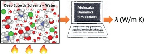
Accurate knowledge and control of thermal conductivities is central for the efficient design of heat storage and transfer devices working with deep eutectic solvents (DESs). The addition of water is a straightforward and cost-efficient way of tuning many properties of DESs. In this work, the thermal conductivities of aqueous solutions of reline, ethaline, and glyceline are reported for the first time. The non-equilibrium molecular dynamics Müller-Plathe (MP) method was used, along with the well-established GAFF and SPC/E force fields for DESs and water, respectively. We show that thermal conductivities of neat DESs are in excellent agreement with available experimental data. The addition of 25 wt% water results in nearly 2 times higher thermal conductivities in all DESs. A further increase in the fraction of water to 75 wt%, causes an increase in the thermal conductivities of DESs ca. 3 times. This behaviour is mainly due to the change in the microscopic structure of the DESs (i.e. hydrogen bonding) upon the addition of water. Our simulations reveal that thermal conductivities of aqueous DESs do not significantly depend on temperature. We also show that thermal conductivities strongly depend on system-size. System-sizes bigger larger than ca. 5 nm should be used.

GRAPHICAL ABSTRACT

Keywords:

• Thermal conductivity
• deep eutectic solvents
• molecular dynamics simulation
• aqueous solutions
• temperature effects

1. Introduction

Sustainable, efficient, and cost-effective heat transfer fluids are essential for a wide variety of industrial and domestic applications such as solar power generation [1, 2], heat storage in power plants [3], high-temperature processing of plastics [4], refrigeration systems [5], and cryogenic gas processing [6, 7]. The conventional organic solvents used in these processes, e.g. benzene, chloroform and toluene, often exhibit non-desirable properties such as high-toxicity and/or high-volatility [8, 9]. To this purpose, the demand for non-hazardous solvents with tailored properties is great. Deep Eutectic Solvents have emerged as a new generation of environmentally-friendly solvents, which can be tuned to exhibit enhanced physical properties [10–12].

DESs are mixtures of a Hydrogen Bond Acceptor (HBA) (e.g. choline chloride, tetrabutylammonium bromide) and a Hydrogen Bond Donor (HBD) (e.g. urea, malonic acid, glycerol) in specific ratios. DESs are liquids having melting points considerably lower than the ones of the building blocks used for their synthesis [13–16]. Properties such us the low volatility, low vapour pressure, large liquid range, large heat capacity, high thermal stability, and non-flammability, make DESs very promising working fluids in high-temperature applications [13, 17–19]. Depending on the nature of the building blocks used, DESs can be biodegradable, bio-compatible, and non-toxic [20–22]. For this reason, DESs can be also used in low-temperature refrigeration systems [23], and in the pharmaceutical industry [24]. The relatively low-cost of the starting materials and the easy synthetic pathway may enable large-scale industrial production of DESs [21].

The accurate prediction of the thermal conductivities of DESs is crucial for the safe and efficient design of heat transfer processes and devices working with DESs (e.g. chemical reactors, heat exchangers, thermal storage units) [25–27]. Thermal conductivity is a measure for the amount of heat that is transferred through a material due to a temperature gradient [25, 26]. Despite being a key property, only a very limited number of studies in literature have focussed on the thermal conductivity of DESs. Recently, the thermal conductivities of choline chloride (ChCl)/urea [26], ChCl/glycerol [28, 29], and ChCl/ethylene glycol [30] have been measured experimentally at different temperatures. It was shown that ChCl-based DESs have relatively low thermal conductivities that do not strongly depend on temperature. The low thermal conductivities, combined with the high viscosities, present a significant advantage for many practical applications of DESs, for example, as a thermal barrier (i.e. insulating materials) in devices that fail due to overheating [31]. A low thermal conductivity is also considered to be a limitation in the efficiency of heat transfer devices such as heat sinks in electronics [32]. To this purpose, tailor-designed DESs having thermal conductivities that can satisfy certain applications is pivotal. A relatively easy and cost-effective way to tune the thermodynamic and transport properties of DESs is by adding controlled amounts of water [33–35]. As shown by Shah and Mjalli [34], Celebi et al. [35], Fetisov et al. [36], and Kumari et al. [37], the addition of water significantly changes the molecular structure of DESs (i.e. hydrogen bond network). As a result, a number of properties of DESs such as the densities [6, 33, 34, 38–41], viscosities [6, 33, 34, 38–40, 42–44], diffusivities [6, 34, 35, 44], ionic conductivities [34, 35, 40], speed of sound [34, 42], and solubilities [16, 45, 46] are vastly affected, depending on the water content in the mixture.

To the best of our knowledge, no experimental or computational work in literature has focussed on the thermal conductivities of aqueous DESs solutions. To this end, we present new data for the thermal conductivities of aqueous reline, ethaline, and glyceline solutions computed using non-equilibrium molecular dynamics (NEMD) for a wide range of mass fractions of water. The temperature-dependence of thermal conductivities of neat and aqueous glyceline solutions for temperatures ranging from 283.15 to 363.15 K is also shown. A detailed discussion of the effects of the system size, and the length of the swap integral in the MP method on the computation of thermal conductivities is also provided. The remainder of the paper is organised as follows: In Section 2, the description of the used force fields, simulation details, and the MP method are presented. Our main findings are presented in Section 3. Finally, conclusions are discussed in Section 4.

2. Model and method

2.1. Force fields

The generalised amber force field (GAFF) was used to model reline, ethaline, and glyceline [47]. The partial atomic charges were derived via the Restrained Electrostatic Potential (RESP) method [48–50], using the Hartree-Fock HF/6.31G* level of theory [49]. The partial charges of ChCl in reline were uniformly scaled by a factor of 0.8 [49, 51]. The partial charges of ChCl in ethaline and glyceline were uniformly scaled by a factor of 0.9 [51]. As discussed in detail in the studies of Perkins et al. [49, 51] and Liu et al. [18], charge scaling in ILs and DESs is essential because electrostatic interactions are usually overpredicted. Recently, Blazquez et al. [52] showed that the scaling of charges of even simple electrolytes such as NaCl can lead to an improved prediction of the salting out effect of methane in water. In the past few years, various studies have shown that simulations using the GAFF force field combined with scaled charges yield relatively accurate thermodynamic and transport properties of neat reline, ethaline, and glyceline [6, 16, 34, 35, 49, 51, 53].

Water was modelled using the rigid three-site SPC/E force field [54]. SPC/E has been shown to be accurate in predicting the transport properties of pure water [55, 56], and mixtures of water with gases [57] for a wide range of temperatures. The SPC/E force field has been also widely used to model aqueous NaCl solutions [58–63], and aqueous solutions of ionic liquids (ILs) and DESs [6, 34, 64]. In the case of DESs, the combination of GAFF and SPC/E force fields have been shown to yield good agreement with experiments for several thermodynamic and transport properties of aqueous reline, ethaline, and glyceline solutions such as viscosities, diffusivities, ionic conductivities, and thermal expansivities [6, 34, 35]. For all simulations of argon (i.e. for the system size dependence study of thermal conductivity) the parameters of Ghorbanian et al. [65] are used. All force field parameters and charges used in our simulations are listed in Tables S1–S13 of the Supplementary Material.

To further validate the performance of the chosen force fields, we performed equilibrium molecular dynamics (EMD) simulations to compute the densities of aqueous DES solutions. These values were compared to the available experimental data [33, 38, 39]. As can be seen in Figure S4 of the Supplementary Material, the computed densities are in good agreement with the experimental values (deviations are at most 1.5%). It is important to note that the scope of this work is not to exhaustively evaluate the performance of force field combinations, but to investigate the underlying molecular phenomena affecting the thermal conductivity of aqueous DES solutions, and provide new reliable data.

2.2. Molecular dynamics simulation details

MD simulations were carried out in a cubic simulation box, with periodic boundary conditions applied in all directions. Initial configurations of aqueous reline, ethaline, and glyceline solutions were generated using the Packmol software [66]. For each DES, eutectic compositions with a 1:2 molar ratios were used, in which 1 refers to the HBA, and 2 refers to the HBD [67]. To study the effect of water content on the thermal conductivity of the aqueous DES solutions, the mass fraction of water (${\omega }_{\mathrm{w}}$) was varied according to: (1) ${\omega }_{\mathrm{w}}=\frac{N_{\mathrm{w}}{M}_{\mathrm{w}}}{N_{\mathrm{ChCl}}{M}_{\mathrm{ChCl}}+N_{\mathrm{HBD}}{M}_{\mathrm{HBD}}+N_{\mathrm{w}}{M}_{\mathrm{w}}}$(1) where $M_i$ and $N_i$ are the molecular weight and the number of molecules of species i (i.e. ChCl, HBD, and water), respectively. In this study, ChCl is considered to be a single component. In all simulations, the system sizes correspond to simulation boxes equal to ca. 5.5 nm. This was determined by systematically increasing the simulation box lengths until no significant variations in the computed thermal conductivities of DESs are present. A detailed analysis of the system size dependence of thermal conductivities is provided in Section 3.2. A list of all simulated systems can be found in Table S14 of the Supplementary Material.

All MD simulations were performed using the open-source Large-scale Atomic/Molecular Massively Parallel Simulator (LAMMPS), version released on August, 2018 [68]. For integrating Newton's equations of motion, the Verlet algorithm was used with a time step of 1 fs. Long-range electrostatic interactions between charged species were handled using the particle-particle, particle-mesh (pppm) solver with a root-mean precision of ${10}^{-5}$ [69]. The cut-off distance was set to 12 Å, for both Lennard-Jones (LJ) and the real-space part of electrostatic interactions. The LJ parameters for the interaction between dissimilar atoms were obtained using the Lorentz–Berthelot combining rules [70]. For water molecules, bond lengths and bond-bending angles were kept fixed using the SHAKE algorithm [71].

The simulation scheme used in all systems is described in the following steps:

1. Initial configurations were energy minimised for 10,000 steps using the conjugate gradient method.

2. EMD simulations of 1 ns in the isothermal-isobaric (NPT) ensemble were performed for the equilibration of the systems. The temperature and pressure were kept constant using the Nosé-Hoover thermostat and barostat with coupling constants of 0.1 ps and 1 ps, respectively.

3. NPT runs of 4 ns are performed for computing the average volumes and densities. The densities of all simulated aqueous DES solutions are listed in Table S15 of the Supplementary Material along with the respective experimental values.

4. Starting from the average densities obtained in the previous step, each system was further equilibrated for 1 ns in the canonical (NVT) ensemble. The temperature was kept constant using the Nosé-Hoover thermostat with a coupling constant of 0.1 ps.

5. NEMD production runs of 50 ns in the NVT ensemble were performed for computing the thermal conductivities using the MP method [72]. The MP method is discussed in detail in the following section. The standard deviation of the computed thermal conductivities are obtained from 6 independent simulations, each one starting from a different initial configuration.

2.2.1. Müller-Plathe (MP) method for computing thermal conductivities

Thermal conductivities can be computed by NEMD and EMD simulations. In NEMD, the response of the system to an externally induced heat flux, or an imposed temperature gradient, yields the thermal conductivity [72–77]. In EMD, two equivalent methods can be used, i.e. the Green-Kubo (GK) [73, 78–81] or Einsten relations [31, 82–84]. It is important to note that both EMD methods require the heat flux vector J for computing thermal conductivities [73]. As shown in the recent studies by Surbyls et al. [85] and Boone et al. [86], the computation of J in molecular simulation packages such as LAMMPS can be erroneous for molecular systems having angles, torsions, dihedrals, and improper dihedrals, producing unphysical values. In fact, our preliminary thermal conductivity computations for reline using the Einstein method (OCTP plugin in LAMMPS [84]) yielded values which were almost an order of magnitude higher than the respective experiments. Therefore, in this study, the MP method was used. The MP method [72] is based on NEMD simulations and has been extensively used for computing thermal conductivities of fluid models, e.g. Lennard-Jones (LJ) particles [72, 87], as well of a wide variety of molecular fluids and liquid mixtures, e.g. water, hydrocarbons and ionic liquids (ILs) [18, 67, 88, 89]. A brief description of the MP method for computing thermal conductivity is as follows: A heat flux is induced to the system by exchanging kinetic energies between the hottest and coldest particles in different regions of the simulation box. Energies are exchanged with a swap integral W (in units of time). As we discuss in detail in the Section 3.1, the choice of W governs the magnitude of the heat flux (and of the resulting temperature gradient). The time-averaged heat flux $⟨J_z(t)⟩$ is described by: (2) $⟨J_z(t)⟩=\frac{\sum _{\mathrm{transfers}}\frac{m}{2}(v_{\mathrm{hot}}^2-v_{\mathrm{cold}}^2)}{2t{L}_{\mathrm{x}}{L}_{\mathrm{y}}}$(2) where the sum is taken over all energy transfers during the simulation time t. $v_{\mathrm{cold}}$ and $v_{\mathrm{hot}}$ denote the velocities of the cold and hot atoms. The mass of the exchanged atoms are represented by m. The product $L_x{L}_y$ is the cross-sectional area in which heat transport occurs and z is the direction of the temperature gradient. The factor 2 in the denominator is due to the periodicity, indicating that energy can be transferred in two directions. The velocity exchange increases the local temperature of the hot slab while decreasing the local temperature of the cold slab. Since the total energy is conserved, this velocity exchange eventually creates a temperature gradient $\mathrm{d}T/\mathrm{d}z$ in the system. The temperature gradient is computed by linear regression of local temperatures in the flow direction for each half of the simulation box. The thermal conductivity (λ) is computed by the ratio of the imposed heat flux to the resulting temperature: (3) $\lambda =-\frac{⟨J_z(t)⟩}{⟨\mathrm{d}T/\mathrm{d}z⟩}$(3) where the brackets $⟨\cdots ⟩$ denote a time average.

3. Results and discussion

In this section, our findings for various aspects that can affect the thermal conductivity of aqueous DESs solutions are presented. We discuss the effect of the swap integral in the MP method, system size effects, the effect of water content, and the temperature dependence of thermal conductivity.

3.1. The effect of the swap integral in the MP method

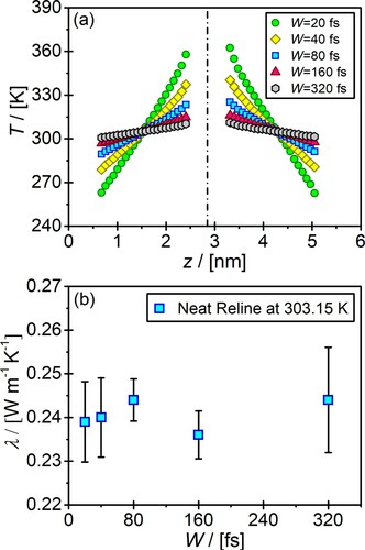
In the MP method, the generated heat flux (and thus the resulting temperature gradient) strongly depends on the choice of the swap interval W [72]. To investigate the effect of W on the computation of thermal conductivities of aqueous DESs solutions, we performed simulations for different values of W . In Figure 1(a), the resulting temperature profiles as a function of distance in the z-direction (i.e. the direction of the temperature gradient) are shown for W = 20, 40, 80, 160 and 320 fs for neat reline. The temperature gradient decreases as W increases. For the lowest value of W tested (i.e. 320 fs) a temperature difference of 10 K between the hot and cold regions is obtained. In contrast, for low values of W (i.e. $W=25\mathrm{fs}$), the temperature difference between the hot and cold regions equals ca. 100 K. For the other values of W , the temperature difference between hot and cold regions lie between these two values. As shown in the studies by Müller-Plathe [72] and Sirk et al. [88], sufficiently high values of W are essential to generate large enough heat fluxes (and the resulting temperature gradients). The value of W should be low enough to ensure that linear response theory still holds (i.e. linear temperature profiles are obtained). Consequently, a proper selection of W is important to minimise the error in the computed thermal conductivities due to the linear regression of the temperature profiles. In Figure 1(b), we show that the computed thermal conductivities for different values of W are practically identical within the error bars. No significant differences in the computation time of the thermal conductivities were observed by using the different values of W . The smallest error (i.e. 2%) in the computed thermal conductivity is observed for $W=80\mathrm{fs}$. For this reason, $W=80\mathrm{fs}$ is used in all the remainder simulations in this work.

Figure 1. The effect of swap integral on the (a) resulting temperature gradient, and (b) computed thermal conductivities of neat reline solutions at 303.15 K and 1 atm.

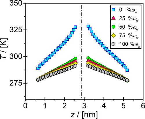
The presence of water in the DES solution also effects the magnitude of the computed temperature gradient. In Figure 2, the temperature gradient of aqueous reline solutions at 303.15 K and 1 atm are shown as a function of distance in z-direction for different water contents using $W=80\mathrm{fs}$. It is clear that the temperature gradient decreases the water content in the solution increases. The temperature difference between the hot and the cold regions for the neat reline and neat water are 45 K and 15 K, respectively. For the rest of the mass fractions of water, the temperature difference between the hot and cold regions are between these two values. These profiles are adequate for linear regression, and thus, a precise computation of thermal conductivity. This further justifies the choice of $W=80\mathrm{fs}$.

Figure 2. Temperature gradients of aqueous reline solutions at 303.15 K and 1 atm as a function of distance in z-direction for mass fractions of water ranging from 0 to 100%. $W=80\mathrm{fs}$ is used in all simulations.

3.2. The effect of the system size on thermal conductivities of aqueous DESs

In molecular simulations, the computation of various transport and thermodynamic properties such as the self- and collective diffusivities [83, 90–93], Kirkwood-Buff integrals [94–97], activity coefficients [98], and ionic conductivities [99] strongly depends on the system size. This is mainly due to the use of periodic boundary conditions, and the long-range nature of hydrodynamic and electrostatic interactions [100, 101]. To mitigate these finite-size effects, the use of relatively large system sizes or the use of analytic corrections is crucial. Thermal conductivities computed with the MP method also exhibit finite-size effects [88, 102]. Sellan et al. [102] showed that these effects become significant when the size of the simulation box is smaller than the mean-free path of the phonons.

In Figure 3, the effect of system size on the computed thermal conductivities of liquid argon at 86 K and 1 atm (which corresponds to an average density of $1403{\mathrm{kg}/\mathrm{m}}^3$), and neat reline at 303.15 K and 1 atm (which corresponds to an average density of $1212{\mathrm{kg}/\mathrm{m}}^3$) are shown. Argon was used as a test-case because it is very computationally efficient (i.e. modelled as a single LJ interaction site) allowing for the investigation of big system sizes. The largest system size of argon in this work is 571,787 molecules, which corresponds to a simulation box length ($L_c$) of ca. 30 nm. Performing simulations with similar box lengths for reline is very computationally intensive. The largest tested system size for reline is 1575 molecules, which corresponds to a simulation box of ca. 8 nm. For both argon and reline, the computed thermal conductivities initially increase with the system size until converging to a plateau at a system size of ca. 5 nm, which corresponds to systems containing more than 2000 and 400 argon and reline molecules, respectively. As shown in Figure 3, the computed thermal conductivities (for system sizes at which the plateau is reached) of both argon and reline are in good agreement with experimental results, showing a deviation of ca. 5%. Based on this investigation, all simulations for the computation of thermal conductivities are performed using system sizes corresponding to simulation box lengths of 5.5 nm. The number of molecules used in each simulation is listed in Table S16 in the Supplementary Material.

Figure 3. System size dependence of computed thermal conductivities of (a) liquid argon at 86 K and 1 atm ($\rho =1403{\mathrm{kg}/\mathrm{m}}^3$), and (b) neat reline at 303.15 K and 1 atm ($\rho =1212{\mathrm{kg}/\mathrm{m}}^3$). $N_{\mathrm{Ar}}$ and $N_{\mathrm{R}}$ are the number of argon and reline molecules, respectively. The red dotted lines refer to experimental data for argon [119] and reline [26]. The dashed lines connecting the symbols are to guide the eye.

3.3. The effect of the water content on thermal conductivities of aqueous DESs

In Figure 4, the computed thermal conductivities of aqueous reline, ethaline, and glyceline solutions at 303.15 K are shown as a function of the mass fraction of water. To the best of our knowledge, no experimental measurements of the thermal conductivity of aqueous DES solutions are available, while a few are reported for the neat DESs [26, 28–30]. As shown in Figure 4, computed thermal conductivities of neat reline, ethaline, and glyceline, are equal to $0.244\mathrm{W}\cdot {\mathrm{m}}^{-1}{\mathrm{K}}^{-1}$, $0.228\mathrm{W}\cdot {\mathrm{m}}^{-1}{\mathrm{K}}^{-1}$, and $0.237\mathrm{W}\cdot {\mathrm{m}}^{-1}{\mathrm{K}}^{-1}$, respectively. These results are in good agreement with the available experiments, i.e. the thermal conductivities of neat reline at 298 K and neat glyceline at 305 K were reported to be $0.245\mathrm{W}\cdot {\mathrm{m}}^{-1}{\mathrm{K}}^{-1}$ and $0.232\mathrm{W}\cdot {\mathrm{m}}^{-1}{\mathrm{K}}^{-1}$, respectively [26, 29]. Interestingly, the thermal conductivities of many common ILs, such as [EMIM][OAc], [BBIM][NTf${}_2$] [C${}_2$mim][EtSO${}_4$], and [C${}_4$mim][Tf${}_2$N] are in the range of 0.11 and $0.23\mathrm{W}\cdot {\mathrm{m}}^{-1}{\mathrm{K}}^{-1}$ [18, 89, 103, 104]. Nevertheless, the thermal conductivities of DESs and ILs are much lower compared to the ones of aqueous solutions of simpler electrolytes such as NaCl, LiBr, and CoCl${}_2$ which are in the range $0.5--0.7\mathrm{W}\cdot {\mathrm{m}}^{-1}{\mathrm{K}}^{-1}$ [105–107].

Figure 4. The thermal conductivities of aqueous reline, ethaline, and glyceline solutions at 303.15 K and 1 atm as a function of the mass fraction of water. The symbol × represents the computed thermal conductivity of the quaternary mixture of reline+etaline+glyceline+water in which each component has a mass fraction of 25 wt%. BlUe, green and red lines (dashed and solid) represent the fit using the Jamieson correlation (Equation (4(4) ${\lambda }_m={\omega }_1{\lambda }_1+{\omega }_2{\lambda }_2-\alpha ({\lambda }_2-{\lambda }_1)[1-(\sqrt{{\omega }_2})]{\omega }_2$(4) )) for reline, glyceline and ethaline, respectively [25]. The uncertainties in the computed thermal conductivities are in the range of 1–3%.

As shown in Figure 4, the thermal conductivities of the aqueous DES solutions increase with the increase in the water content. This can be explained by the changes in the micro-structure of the DESs in the presence of water. As shown in previous studies [6, 34–37], with the addition of water, hydrogen bonds (HB) between HBDs and anions, and between anions are significantly reduced while new HBs between the water molecules and the ions are formed. Moreover, water reduces the viscosity of the mixture, and thus, the self-diffusivities of all species increase along with the thermal conductivities [108, 109]. More details on the variation of the HBs and self-diffusivities as a function of the water content can be found in the studies by Baz et al. [6] and Celebi et al. [35].

In this study, our computed thermal conductivity of the SPC/E water model is equal to $0.853\mathrm{W}\cdot {\mathrm{m}}^{-1}{\mathrm{K}}^{-1}$ (see Figure 4). This value is in agreement with earlier results for the same force field computed either using the MP [67, 88, 110, 111] or the Green-Kubo method [88, 112, 113]. The thermal conductivity of the rigid SPC/E water model at 303.15 K deviates from the experimentally measured one (i.e. $0.615\mathrm{W}\cdot {\mathrm{m}}^{-1}{\mathrm{K}}^{-1}$) by ca. 35%. Therefore, given the good performance of the GAFF force field in predicting the thermal conductivity of neat DESs, and the lower accuracy of the SPC/E force field for water, it is reasonable to expect that the computed thermal conductivities of the aqueous DES solutions will deviate from the actual thermal conductivities by not more than 35%, depending on the water content in the mixture. It is important to note that such overestimations of the thermal conductivity of water were also reported by many previous MD studies for various water force fields (i.e. 3-site, 4-site, flexible, and rigid) [67, 88, 110–113]. In these studies it is shown that none of the considered water force fields can accurately reproduce the experimentally measured thermal conductivity. Despite this deviation, it is important to note that our findings for the dependence of thermal conductivity of the aqueous DES solutions on the water content are in qualitative agreement with prior experimental and simulation studies on aqueous ILs solutions. Ge et al. [104] performed experiments to determine the effect of water content on the thermal conductivities of aqeuous solutions of [C${}_2$mim][EtSO${}_4$] and [C${}_2$mim][OTf] at 293 K. Kelkar et al. [114] performed MD simulations of aqueous [C${}_2$mim][EtSO${}_4$] solutions. In both studies, an increase in the thermal conductivities was obtained with increasing water content.

As can be seen in Figure 4, the computed thermal conductivities of the aqueous reline solutions are slightly, but consistently, higher than the respective ones of the aqueous glyceline and ethaline solutions for the whole range of water mass fractions [35]. These small differences can be mainly explained by the different H-bonding behaviour of the three DESs due to the variation in the HBDs, i.e. urea in reline, ethylene glycol in ethaline and glycerol in glyceline [6, 35]. Urea is a strong HBD, which has been experimentally shown to be associated with high thermal conductivities. Gautham and Seth [26] measured the thermal conductivities of ChCl/urea and ChCl/thio-urea and showed that ChCl/urea has higher thermal conductivity due to the stronger H-bonding nature of urea (i.e. the electronegativity of oxygen in urea is higher than sulfur in thio-urea). Our results also show that the thermal conductivities of aqueous glyceline solutions are slightly higher than those of ethaline. This is consistent with the experimentally measured thermal conductivities of the neat glycerol and etyhlene glycol. The measured thermal conductivity of glycerol ($0.292\mathrm{W}\cdot {\mathrm{m}}^{-1}{\mathrm{K}}^{-1}$) is slightly higher than the one of ethylene glycol ($0.256\mathrm{W}\cdot {\mathrm{m}}^{-1}{\mathrm{K}}^{-1}$) at 298.15 K [115] In this study, we also simulated a quaternary mixture of reline-ethaline-glyceline-water with equal mass fractions. We aimed to diversify HB networks using three different DESs in an aqueous solution, and investigate how this affects the thermal condutivities. The computed thermal conductivitiy of the quaternary mixture is equal to $0.413\mathrm{W}\cdot {\mathrm{m}}^{-1}{\mathrm{K}}^{-1}$. As can be clearly seen in Figure 4, this value is nearly identical to the thermal conductivity of glyceline solution having mass fraction of water of 25 wt%, which lies between the thermal conductivities of reline and ethaline solutions for the same water content. This finding clearly shows that the thermal conductivities of DESs can be accurately tuned by adjusting the compositions in their mixtures. All raw data and the corresponding uncertainties are listed in Table S17 of the Supplementary Material.

Several empirical models such as the Flippov equation [25], Jamieson correlation [116], Baroncini correlation [25, 116], and Rowley method [117] have been proposed for predicting thermal conductivities of liquid mixtures from pure component data. Jamieson correlation [116] was validated using the thermal conductivities of a wide range of aqueous and non-aqueous binary mixtures for various compositions. These mixtures involved ethers, ketones, alcohols, aromatics, weak acids, water, saccharides, milk, butter, whey, and fruit juices. Jamieson correlation is as follows: (4) ${\lambda }_m={\omega }_1{\lambda }_1+{\omega }_2{\lambda }_2-\alpha ({\lambda }_2-{\lambda }_1)[1-(\sqrt{{\omega }_2})]{\omega }_2$(4) where ${\lambda }_m$ is the thermal conductivity of the binary mixture of components 1 and 2, having thermal conductivities ${\lambda }_1$ and ${\lambda }_2$, respectively. The two components are sorted so that ${\lambda }_2>{\lambda }_1$. $w_1$ and $w_2$ are the mass fractions of components 1 and 2, respectively. α is an empirical parameter that is temperature-independent and can be obtained by fitting to the available experimental data. According to Jamieson et al. [116], the thermal conductivity of any binary mixture (aqueous or non-aqueous) can be predicted with a minimum accuracy of 7% by Equation (4(4) ${\lambda }_m={\omega }_1{\lambda }_1+{\omega }_2{\lambda }_2-\alpha ({\lambda }_2-{\lambda }_1)[1-(\sqrt{{\omega }_2})]{\omega }_2$(4) ) with $\alpha =1$ (if no experimental data are available to fit).

Although Jamieson correlation was not developed considering aqueous electrolyte solutions, it has been used earlier to predict the thermal conductivities of such systems. Ge et al. [104], validated Equation (4(4) ${\lambda }_m={\omega }_1{\lambda }_1+{\omega }_2{\lambda }_2-\alpha ({\lambda }_2-{\lambda }_1)[1-(\sqrt{{\omega }_2})]{\omega }_2$(4) ) using the thermal conductivities of aqueous solutions of [C${}_2$mim][EtSO${}_4$] and [C${}_2$mim][OTf] ILs. These authors showed that by using fitted α parameters equal to 0.4211 and 0.7043, respectively, Equation (4(4) ${\lambda }_m={\omega }_1{\lambda }_1+{\omega }_2{\lambda }_2-\alpha ({\lambda }_2-{\lambda }_1)[1-(\sqrt{{\omega }_2})]{\omega }_2$(4) ) is able to predict the thermal conductivities very accurately. Fitting the data by Ge et al. [104] using the general rule proposed by Jamieson et al. [116], i.e. $\alpha =1$, yields thermal conductivities with accuracy in the range of 1.7–14.8%. Excluding the mass fractions of water equal to 20 wt% and 50 wt%, the predictions of thermal conductivities show an accuracy in the range of 1.7–6.6%. This clearly shows that Jamieson correlation can be safely used to predict the thermal conductivities of aqueous ILs solutions, even by using a fixed value of $\alpha =1$.

As shown in Figure 4, the computed data for the aqueous DESs solutions are fitted using the Jamieson correlation (Equation (4(4) ${\lambda }_m={\omega }_1{\lambda }_1+{\omega }_2{\lambda }_2-\alpha ({\lambda }_2-{\lambda }_1)[1-(\sqrt{{\omega }_2})]{\omega }_2$(4) )). Values of fitted α parameters equal to −0.61, −0.22 and 0, for reline, glyceline and ethaline solutions, respectively, yield a very good fit of the Jamieson correlation to the computed thermal conductivities. The thermal conductivity of aqueous ethaline is an almost linear function of the mass fraction of water, and thus, $\alpha =0$ in this case. In Figure 4, we also fit the computed data using $\alpha =1$. The use of $\alpha =1$ does not yield accurate predictions for the thermal conductivities of the aqueous DESs solutions, showing deviations from the computed data in the range of 8.8–30.4%. Interestingly, if the fitted α parameters are used, the Jamieson correlation is a concave function, while the use of $\alpha =1$ produces a convex function of the thermal conductivities with the mass fraction of water. These findings clearly show that the general rule of thumb proposed by Jamieson et al. (i.e. $\alpha =1$) does not hold for the prediction of thermal conductivities of aqueous DESs solutions, and hence new models may be needed.

3.4. The effect of the temperature on thermal conductivities of aqueous DESs

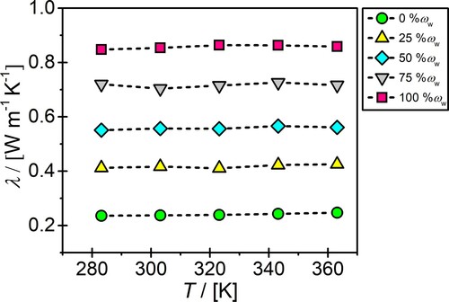
Figure 5 shows the computed thermal conductivities of aqueous glyceline solutions for temperatures in the range of 283.15–363.15 K, and mass fractions of water from 0 (i.e. neat glyceline) to 100 wt% (i.e. neat water). For the whole range of mass fractions of water, it is evident that the thermal conductivities do not depend on the temperature. This can be mainly explained by the negligible change in the microstructure of aqueous DESs (and neat water) with the increase in temperature. As recently shown by Celebi et al. [35], the radial distribution functions and the HB networks between the components of aqueous reline and ethaline solutions do not significantly change as a function of temperature. These findings are also in line with several earlier experimental measurements for different DESs [26, 29, 30], and MD studies and experiments for many common ILs [18, 89, 103, 104, 118]. The thermal conductivities of ILs showed a small decrease with the increase in temperature [18, 89, 103, 104, 118]. In contrast, the experimental study by Singh et al. [28] revealed that a temperature increase of ${80}^{\circ }\mathrm{C}$ results in a more than 10% increase in the thermal conductivity of neat glyceline. As shown in Figure 5, for the same system a temperature increase from 283.15 to 363.15 K results in 4% increase in the thermal conductivity. Note that this difference is within the uncertainty range (see Table S18 of the Supplementary Material).

Figure 5. The effect of temperature on the computed thermal conductivities of aqueous glyceline solutions with water mass fractions ranging from 0 to 100%. The uncertainties in the computed thermal conductivities are in the range of 1–3%. The dotted lines connecting the symbols are to guide the eye.

4. Conclusions

We performed molecular dynamics simulations using the Müller-Plathe method [72] to compute thermal conductivities of aqueous solutions of reline, ethaline, and glyceline DESs at 303.15 K, and mass fractions of water ranging from 0 to 100 wt%. To the best of our knoweledge, no available experimental or simulation data are available for the aqueous DESs mixtures. The GAFF and SPC/E force fields were used for modelling DESs and water, respectively. Our findings for neat DESs show a good agreement with available experimental data, deviating by a maximum of 3%. With the addition of 25 wt% water, thermal conductivities of all DESs increase by almost a factor of 2 (i.e. 1.9 for reline, 1.8 for glyceline, and 1.7 for ethaline). For 75 wt% water, the thermal conductivities increase ca. 3 times. This behaviour is mainly related to the depletion of hydrogen bonds between the components of DESs, and the formation of new ones, between the water molecules and DESs. The differences between the computed thermal conductivities of the three DESs are mainly due to the hydrogen bonding ability of urea, ethylene glycol, and glycerol. Our simulations revealed that the influence of temperature on the thermal conductivities of the aqueous solutions of DESs is negligible. For the aqueous glyceline solutions, the computed thermal conductivities at 283.15 K are ca. 4% lower than the ones at 363.15 K for the whole range of mass fractions of water. We also investigated the dependence of the computed thermal conductivities on the simulation system size using argon and reline as test cases. The thermal conductivities of both systems showed an initial increase with the system size until reaching a constant value for system sizes corresponding to simulations box lengths of ca. 5 nm. The effect of the swap integral in the Müller-Plathe method was also studied. Although the swap integral governs the magnitude of the heat flux, we show that all values in the range of 20–320 fs yield practically identical thermal conductivities. Nevertheless, the small and large values cause relatively large errors in the computed thermal conductivities. Therefore, the use of an intermediate swap integral, e.g. 80 fs, is advised for molecular simulations of aqueous DESs solutions.

Acknowledgements

This study was funded by Nederlandse Organisatie voor Wetenschappelijk Onderzoek within the framework of NWO Exacte Wetenschappen (Physical Sciences) for the use of high-performance computing facilities. TJHV acknowledges NWO-CW (Chemical Sciences) for a VICI grant.

Disclosure statement

No potential conflict of interest was reported by the author(s).

Additional information

Funding

This study was funded by Nederlandse Organisatie voor Wetenschappelijk Onderzoek within the framework of NWO Exacte Wetenschappen (Physical Sciences) for the use of high-performance computing facilities. TJHV acknowledges NWO-CW (Chemical Sciences) for a VICI grant [NWO-CW,NWO-EW].

References

- K. Vignarooban, X. Xu, A. Arvay, K. Hsu and A.M. Kannan, Appl. Energy 146, 383–396 (2015). doi:https://doi.org/10.1016/j.apenergy.2015.01.125.
- B. Wu, R.G. Reddy and R.D. Rogers, in International Solar Energy Conference, Vol. 16702. (American Society of Mechanical Engineers, Washington DC, 2001), pp. 445–451.
- D. Brosseau, J.W. Kelton, D. Ray, M. Edgar, K. Chisman and B. Emms, J. Sol. Energy. Eng. 127 (1), 109–116 (2005). doi:https://doi.org/10.1115/1.1824107.
- Y. Naresh, A. Dhivya, K. Suganthi and K. Rajan, Nanosci. Nanotechnol. Lett. 4 (12), 1209–1213 (2012). doi:https://doi.org/10.1166/nnl.2012.1454.
- H. Peng, G. Ding, W. Jiang, H. Hu and Y. Gao, Int. J. Refrig. 32 (6), 1259–1270 (2009). doi:https://doi.org/10.1016/j.ijrefrig.2009.01.025.
- J. Baz, C. Held, J. Pleiss and N. Hansen, Phys. Chem. Chem. Phys. 21 (12), 6467–6476 (2019). doi:https://doi.org/10.1039/C9CP00036D.
- J. Singh, Heat Transfer Fluids and Systems for Process and Energy Applications, 1st ed. (CRC Press, New York, 2020).
- E. Browning, Toxicity of Industrial Organic Solvents, Vol. 80. (HM Stationery Office, New York, 1953).
- K. Grodowska and A. Parczewski, Acta Pol. Pharm. 67 (1), 3–12 (2010).
- M.E. Van Valkenburg, R.L. Vaughn, M. Williams and J.S. Wilkes, Thermochim. Acta 425 (1–2), 181–188 (2005). doi:https://doi.org/10.1016/j.tca.2004.11.013.
- Q. Zhang, K.D.O. Vigier, S. Royer and F. Jérôme, Chem. Soc. Rev. 41 (21), 7108–7146 (2012). doi:https://doi.org/10.1039/c2cs35178a.
- A. van den Bruinhorst, T. Spyriouni, J.R. Hill and M.C. Kroon, J. Phys. Chem. B 122 (1), 369–379 (2018). doi:https://doi.org/10.1021/acs.jpcb.7b09540.
- E.L. Smith, A.P. Abbott and K.S. Ryder, Chem. Rev. 114 (21), 11060–11082 (2014). doi:https://doi.org/10.1021/cr300162p.
- Y. Liu, J.B. Friesen, J.B. McAlpine, D.C. Lankin, S.N. Chen and G.F. Pauli, J. Nat. Prod. 81 (3), 679–690 (2018). doi:https://doi.org/10.1021/acs.jnatprod.7b00945.
- A.P. Abbott, G. Capper, D.L. Davies, R.K. Rasheed and V. Tambyrajah, Chem. Commun. (1), 70–71 (2003). doi:https://doi.org/10.1039/b210714g.
- H.S. Salehi, M. Ramdin, O.A. Moultos and T.J.H. Vlugt, Fluid Phase Equilib. 497, 10–18 (2019). doi:https://doi.org/10.1016/j.fluid.2019.05.022.
- R. Craveiro, I. Aroso, V. Flammia, T. Carvalho, M.T. Viciosa, M. Dionísio, S. Barreiros, R.L. Reis, A.R.C. Duarte and A. Paiva, J. Mol. Liq. 215, 534–540 (2016). doi:https://doi.org/10.1016/j.molliq.2016.01.038.
- H. Liu, E.J. Maginn, A.E. Visser, N.J. Bridges and E.B. Fox, Ind. Eng. Chem. Res. 51 (21), 7242–7254 (2012). doi:https://doi.org/10.1021/ie300222a.
- L.J.B.M. Kollau, M. Vis, A. van den Bruinhorst, A.C.C. Esteves and R. Tuinier, Chem. Commun. 54 (95), 13351–13354 (2018). doi:https://doi.org/10.1039/C8CC05815F.
- Y. Dai, J. van Spronsen, G.J. Witkamp, R. Verpoorte and Y.H. Choi, Anal. Chim. Acta 766, 61–68 (2013). doi:https://doi.org/10.1016/j.aca.2012.12.019.
- A. Paiva, R. Craveiro, I. Aroso, M. Martins, R.L. Reis and A.R.C. Duarte, ACS. Sustain. Chem. Eng. 2 (5), 1063–1071 (2014). doi:https://doi.org/10.1021/sc500096j.
- D.J.G.P. van Osch, C.H.J.T. Dietz, J. van Spronsen, M.C. Kroon, F. Gallucci, M. van Sint Annaland and R. Tuinier, ACS. Sustain. Chem. Eng. 7 (3), 2933–2942 (2019). doi:https://doi.org/10.1021/acssuschemeng.8b03520.
- R. Abedin, S. Heidarian, J.C. Flake and F.R. Hung, Langmuir 33 (42), 11611–11625 (2017). doi:https://doi.org/10.1021/acs.langmuir.7b02003.
- H. Shekaari and M. Mokhtarpour, J. Adv. Chem. Pharm. Mater. (JACPM) 3 (2), 233–234 (2020).
- B.E. Poling, J.M. Prausnitz and J.P. O'Connell, et al., The Properties of Gases and Liquids, Vol. 5, 5th ed. (Mcgraw-hill New York, New York, 2001).
- R.K. Gautam and D. Seth, J. Therm. Anal. Calorim. 140, 2633–2640 (2020). doi:https://doi.org/10.1007/s10973-019-09000-2.
- R.K. Shah and D.P. Sekulic, Fundamentals of Heat Exchanger Design, 1st ed. (John Wiley & Sons, New York, 2003).
- A. Singh, R. Walvekar, M. Khalid, W.Y. Wong and T. Gupta, J. Mol. Liq. 252, 439–444 (2018). doi:https://doi.org/10.1016/j.molliq.2017.10.030.
- C. Liu, H. Fang, Y. Qiao, J. Zhao and Z. Rao, Int. J. Heat Mass Transf. 138, 690–698 (2019). doi:https://doi.org/10.1016/j.ijheatmasstransfer.2019.04.090.
- Y.C. Yan, W. Rashmi, M. Khalid, K. Shahbaz, T. Gupta and N. Mase, Int. J. Eng. Sci. Technol. 12, 1–14 (2017).
- A. Kınacı, J.B. Haskins, C. Sevik and T. Çağın, Phys. Rev. B 86 (11), 115410 (2012). doi:https://doi.org/10.1103/PhysRevB.86.115410.
- K. Chu, Q. Wu, C. Jia, X. Liang, J. Nie, W. Tian, G. Gai and H. Guo, Compos. Sci. Technol. 70 (2), 298–304 (2010). doi:https://doi.org/10.1016/j.compscitech.2009.10.021.
- A. Yadav, S. Trivedi, R. Rai and S. Pandey, Fluid Phase Equilib. 367, 135–142 (2014). doi:https://doi.org/10.1016/j.fluid.2014.01.028.
- D. Shah and F.S. Mjalli, Phys. Chem. Chem. Phys. 16 (43), 23900–23907 (2014). doi:https://doi.org/10.1039/C4CP02600D.
- A.T. Celebi, T.J.H. Vlugt and O.A. Moultos, J. Phys. Chem. B 123 (51), 11014–11025 (2019). doi:https://doi.org/10.1021/acs.jpcb.9b09729.
- E.O. Fetisov, D.B. Harwood, I.F.W. Kuo, S.E.E. Warrag, M.C. Kroon, C.J. Peters and J.I. Siepmann, J. Phys. Chem. B 122 (3), 1245–1254 (2018). doi:https://doi.org/10.1021/acs.jpcb.7b10422.
- P. Kumari, Shobhna, S. Kaur and H.K. Kashyap, ACS Omega 3 (11), 15246–15255 (2018). doi:https://doi.org/10.1021/acsomega.8b02447.
- A. Yadav and S. Pandey, J. Chem. Eng. Data 59 (7), 2221–2229 (2014). doi:https://doi.org/10.1021/je5001796.
- A. Yadav, J.R. Kar, M. Verma, S. Naqvi and S. Pandey, Thermochim. Acta 600, 95–101 (2015). doi:https://doi.org/10.1016/j.tca.2014.11.028.
- V. Agieienko and R. Buchner, J. Chem. Eng. Data 64 (11), 4763–4774 (2019). doi:https://doi.org/10.1021/acs.jced.9b00145.
- R.B. Leron and M.H. Li, J. Chem. Thermodyn. 54, 293–301 (2012). doi:https://doi.org/10.1016/j.jct.2012.05.008.
- H. Shekaari, M.T. Zafarani-Moattar and B. Mohammadi, J. Mol. Liq. 243, 451–461 (2017). doi:https://doi.org/10.1016/j.molliq.2017.08.051.
- R.B. Leron and M.H. Li, Thermochim. Acta 546, 54–60 (2012). doi:https://doi.org/10.1016/j.tca.2012.07.024.
- C. D'Agostino, L.F. Gladden, M.D. Mantle, A.P. Abbott, I.A. Essa, A.Y. Al-Murshedi and R.C. Harris, Phys. Chem. Chem. Phys. 17 (23), 15297–15304 (2015). doi:https://doi.org/10.1039/C5CP01493J.
- W.C. Su, D.S.H. Wong and M.H. Li, J. Chem. Eng. Data 54 (6), 1951–1955 (2009). doi:https://doi.org/10.1021/je900078k.
- A.C. Dumetz, A.M. Chockla, E.W. Kaler and A.M. Lenhoff, Biophys. J. 94 (2), 570–583 (2008). doi:https://doi.org/10.1529/biophysj.107.116152.
- J. Wang, R.M. Wolf, J.W. Caldwell, P.A. Kollman and D.A. Case, J. Comput. Chem. 25 (9), 1157–1174 (2004). doi:https://doi.org/10.1002/(ISSN)1096-987X.
- C.I. Bayly, P. Cieplak, W. Cornell and P.A. Kollman, J. Phys. Chem. 97 (40), 10269–10280 (1993). doi:https://doi.org/10.1021/j100142a004.
- S.L. Perkins, P. Painter and C.M. Colina, J. Phys. Chem. B 117 (35), 10250–10260 (2013). doi:https://doi.org/10.1021/jp404619x.
- S. Mainberger, M. Kindlein, F. Bezold, E. Elts, M. Minceva and H. Briesen, Mol. Phys. 115 (9-12), 1309–1321 (2017). doi:https://doi.org/10.1080/00268976.2017.1288936.
- S.L. Perkins, P. Painter and C.M. Colina, J. Chem. Eng. Data 59 (11), 3652–3662 (2014). doi:https://doi.org/10.1021/je500520h.
- S. Blazquez, I.M. Zeron, M.M. Conde, J.L.F. Abascal and C. Vega, Fluid Phase Equilib. 513, 112548 (2020). doi:https://doi.org/10.1016/j.fluid.2020.112548.
- H.S. Salehi, R. Hens, O.A. Moultos and T.J.H. Vlugt, J. Mol. Liq. 316, 113729 (2020). doi:https://doi.org/10.1016/j.molliq.2020.113729.
- H.J.C. Berendsen, J.R. Grigera and T.P. Straatsma, J. Phys. Chem. 91 (24), 6269–6271 (1987). doi:https://doi.org/10.1021/j100308a038.
- P. Mark and L. Nilsson, J. Phys. Chem. A 105 (43), 9954–9960 (2001). doi:https://doi.org/10.1021/jp003020w.
- I.N. Tsimpanogiannis, O.A. Moultos, L.F.M. Franco, M.B.M. Spera, M. Erds and I.G. Economou, Mol. Simul. 45 (4–5), 425–453 (2019). doi:https://doi.org/10.1080/08927022.2018.1511903.
- O.A. Moultos, I.N. Tsimpanogiannis, A.Z. Panagiotopoulos and I.G. Economou, J. Phys. Chem. B 118 (20), 5532–5541 (2014). doi:https://doi.org/10.1021/jp502380r.
- A.L. Benavides, M.A. Portillo, J.L.F. Abascal and C. Vega, Mol. Phys. 115 (9-12), 1301–1308 (2017). doi:https://doi.org/10.1080/00268976.2017.1288939.
- G.A. Orozco, O.A. Moultos, H. Jiang, I.G. Economou and A.Z. Panagiotopoulos, J. Chem. Phys. 141 (23), 234507 (2014). doi:https://doi.org/10.1063/1.4903928.
- A.T. Celebi and A. Beskok, J. Phys. Chem. C 122 (17), 9699–9709 (2018). doi:https://doi.org/10.1021/acs.jpcc.8b02519.
- A.T. Celebi, B. Cetin and A. Beskok, J. Phys. Chem. C 123 (22), 14024–14035 (2019). doi:https://doi.org/10.1021/acs.jpcc.9b02432.
- W.R. Smith, I. Nezbeda, J. Kolafa and F. Moučka, Fluid Phase Equilib. 466, 19–30 (2018). doi:https://doi.org/10.1016/j.fluid.2018.03.006.
- I. Nezbeda, F. Moučka and W.R. Smith, Mol. Phys. 114 (11), 1665–1690 (2016). doi:https://doi.org/10.1080/00268976.2016.1165296.
- R.M. Lynden-Bell, Mol. Phys. 101 (16), 2625–2633 (2003). doi:https://doi.org/10.1080/00268970310001592700.
- J. Ghorbanian, A.T. Celebi and A. Beskok, J. Chem. Phys. 145 (18), 184109 (2016). doi:https://doi.org/10.1063/1.4967294.
- L. Martínez, R. Andrade, E.G. Birgin and J.M. Martínez, J. Comput. Chem. 30 (13), 2157–2164 (2009). doi:https://doi.org/10.1002/jcc.v30:13.
- M. Zhang, E. Lussetti, L.E. de Souza and F. Müller-Plathe, J. Phys. Chem. B 109 (31), 15060–15067 (2005). doi:https://doi.org/10.1021/jp0512255.
- S. Plimpton, J. Comput. Phys. 117 (1), 1–19 (1995). doi:https://doi.org/10.1006/jcph.1995.1039.
- S. Plimpton, R. Pollock and M. Stevens, in Proceedings of the Eighth SIAM Conference on Parallel Processing for Scientific Computing, Minneapolis, MN, pp. 1–13.
- M.P. Allen and D.J. Tildesley, Computer Simulation of Liquids, 2nd ed. (Oxford University Press, New York, 2017).
- S. Miyamoto and P.A. Kollman, J. Comput. Chem. 13 (8), 952–962 (1992). doi:https://doi.org/10.1002/(ISSN)1096-987X.
- F. Müller-Plathe, J. Chem. Phys. 106 (14), 6082–6085 (1997). doi:https://doi.org/10.1063/1.473271.
- D. Frenkel and B. Smit, Understanding Molecular Simulation: From Algorithms to Applications, 2nd ed. (Elsevier, San Diego, CA, 2001).
- D.J Evans and G.P Morriss, Statistical Mechanics of Nonequilbrium Liquids, 2nd ed. (Cambridge University Press, Cambridge, 2007).
- T. Ikeshoji and B. Hafskjold, Mol. Phys. 81 (2), 251–261 (1994). doi:https://doi.org/10.1080/00268979400100171.
- J.R. Lukes, D.Y. Li, X.G. Liang and C.L. Tien, J. Heat. Transfer. 122 (3), 536–543 (2000). doi:https://doi.org/10.1115/1.1288405.
- M.P. Lautenschlaeger, M. Horsch and H. Hasse, Mol. Phys. 117 (2), 189–199 (2019). doi:https://doi.org/10.1080/00268976.2018.1504134.
- M.S. Green, J. Chem. Phys. 22 (3), 398–413 (1954). doi:https://doi.org/10.1063/1.1740082.
- R. Kubo, J. Phys. Soc. Jpn 12 (6), 570–586 (1957). doi:https://doi.org/10.1143/JPSJ.12.570.
- G.A. Fernandez, J. Vrabec and H. Hasse, Fluid Phase Equilib. 221 (1-2), 157–163 (2004). doi:https://doi.org/10.1016/j.fluid.2004.05.011.
- S. Sarkar and R.P. Selvam, J. Appl. Phys. 102 (7), 074302 (2007). doi:https://doi.org/10.1063/1.2785009.
- A. Einstein, Ann. Phys. 17 (8), 549–560 (1905). doi:https://doi.org/10.1002/(ISSN)1521-3889.
- S.H. Jamali, L. Wolff, T.M. Becker, A. Bardow, T.J.H. Vlugt and O.A. Moultos, J. Chem. Theory. Comput. 14 (5), 2667–2677 (2018). doi:https://doi.org/10.1021/acs.jctc.8b00170.
- S.H. Jamali, L. Wolff, T.M. Becker, M. de Groen, M. Ramdin, R. Hartkamp, A. Bardow, T.J.H. Vlugt and O.A. Moultos, J. Chem. Inf. Model. 59 (4), 1290–1294 (2019). doi:https://doi.org/10.1021/acs.jcim.8b00939.
- D. Surblys, H. Matsubara, G. Kikugawa and T. Ohara, Phys. Rev. E. 99 (5), 051301 (2019). doi:https://doi.org/10.1103/PhysRevE.99.051301.
- P. Boone, H. Babaei and C.E. Wilmer, J. Chem. Theory. Comput. 15 (10), 5579–5587 (2019). doi:https://doi.org/10.1021/acs.jctc.9b00252.
- C.M. Tenney and E.J. Maginn, J. Chem. Phys. 132 (1), 014103 (2010). doi:https://doi.org/10.1063/1.3276454.
- T.W. Sirk, S. Moore and E.F. Brown, J. Chem. Phys. 138 (6), 064505 (2013). doi:https://doi.org/10.1063/1.4789961.
- H. Liu and E.J. Maginn, J. Chem. Phys. 135 (12), 124507 (2011). doi:https://doi.org/10.1063/1.3643124.
- B. Dünweg and K. Kremer, J. Chem. Phys. 99 (9), 6983–6997 (1993). doi:https://doi.org/10.1063/1.465445.
- I.C. Yeh and G. Hummer, J. Phys. Chem. B 108 (40), 15873–15879 (2004). doi:https://doi.org/10.1021/jp0477147.
- S.H. Jamali, A. Bardow, T.J.H. Vlugt and O.A. Moultos, J. Chem. Theory. Comput. 16 (6), 3799–3806 (2020). doi:https://doi.org/10.1021/acs.jctc.0c00268.
- A.T. Celebi, S.H. Jamali, A. Bardow, T.J.H. Vlugt and O.A. Moultos, Mol. Simul. (2020). In press. doi:https://doi.org/10.1080/08927022.2020.1810685.
- P. Krüger and T.J.H. Vlugt, Phys. Rev. E 97 (5), 051301 (2018). doi:https://doi.org/10.1103/PhysRevE.97.051301.
- P. Krüger, S.K. Schnell, D. Bedeaux, S. Kjelstrup, T.J.H. Vlugt and J.M. Simon, J. Phys. Chem. Lett. 4 (2), 235–238 (2013). doi:https://doi.org/10.1021/jz301992u.
- N. Dawass, P. Krüger, S.K. Schnell, D. Bedeaux, S. Kjelstrup, J.M. Simon and T.J.H. Vlugt, Mol. Simul. 44 (7), 599–612 (2018). doi:https://doi.org/10.1080/08927022.2017.1416114.
- N. Dawass, P. Krüger, S.K. Schnell, O.A. Moultos, I.G. Economou, T.J.H. Vlugt and J.M. Simon, Nanomaterials 10 (4), 771 (2020). doi:https://doi.org/10.3390/nano10040771.
- J.M. Young and A.Z. Panagiotopoulos, J. Phys. Chem. B 122 (13), 3330–3338 (2018). doi:https://doi.org/10.1021/acs.jpcb.7b09861.
- M.J. Klenk and W. Lai, Solid State Ion. 289, 143–149 (2016). doi:https://doi.org/10.1016/j.ssi.2016.03.002.
- C.W. Oseen, Leipzig: Akademische Verlagsgesellschaft mb H. (1927).
- L.R. Pratt and G. Hummer, Simulation and Theory of Electrostatic Interactions in Solution: Computational Chemistry, Biophysics and Aqueous Solutions, Santa Fe, New Mexico, USA, 23-25 June 1999, 1st ed. (American Institute of Physics Inc., New York, 1999).
- D.P. Sellan, E.S. Landry, J. Turney, A.J. McGaughey and C.H. Amon, Phys. Rev. B 81 (21), 214305 (2010). doi:https://doi.org/10.1103/PhysRevB.81.214305.
- A.P. Fröba, M.H. Rausch, K. Krzeminski, D. Assenbaum, P. Wasserscheid and A. Leipertz, Int. J. Thermophys. 31 (11–12), 2059–2077 (2010). doi:https://doi.org/10.1007/s10765-010-0889-3.
- R. Ge, C. Hardacre, P. Nancarrow and D.W. Rooney, J. Chem. Eng. Data 52 (5), 1819–1823 (2007). doi:https://doi.org/10.1021/je700176d.
- I.M. Abdulagatov and U.B. Magomedov, J. Chem. Eng. Jpn 32 (4), 465–471 (1999). doi:https://doi.org/10.1252/jcej.32.465.
- R.M. DiGuilio and A.S. Teja, Ind. Eng. Chem. Res. 31 (4), 1081–1085 (1992). doi:https://doi.org/10.1021/ie00004a016.
- H. Ozbek and S.L. Phillips, J. Chem. Eng. Data. 25 (3), 263–267 (1980). doi:https://doi.org/10.1021/je60086a001.
- S. Mathur and S.C. Saxena, Proc. Phys. Soc. 89 (3), 753 (1966). doi:https://doi.org/10.1088/0370-1328/89/3/331.
- J.T. Edward, J. Chem. Educ. 47 (4), 261 (1970). doi:https://doi.org/10.1021/ed047p261.
- H. Jiang, E.M. Myshakin, K.D. Jordan and R.P. Warzinski, J. Phys. Chem. B 112 (33), 10207–10216 (2008). doi:https://doi.org/10.1021/jp802942v.
- S. Kuang and J.D. Gezelter, J. Chem. Phys. 133 (16), 164101 (2010). doi:https://doi.org/10.1063/1.3499947.
- D. Bertolini and A. Tani, Phys. Rev. E 83 (3), 031202 (2011). doi:https://doi.org/10.1103/PhysRevE.83.031202.
- E.J. Rosenbaum, N.J. English, J.K. Johnson, D.W. Shaw and R.P. Warzinski, J. Phys. Chem. B 111 (46), 13194–13205 (2007). doi:https://doi.org/10.1021/jp074419o.
- M.S. Kelkar, W. Shi and E.J. Maginn, Ind. Eng. Chem. Res. 47 (23), 9115–9126 (2008). doi:https://doi.org/10.1021/ie800843u.
- T.E. Daubert and R.P. Danner, Physical and Thermodynamic Properties of Pure Chemicals: Data Compilation, 8th ed. (Taylor & Francis, Washington, 1997).
- D.T. Jamieson, J.B. Irving and J.S. Tudhope, Liquid Thermal Conductivity: A Data Survey to 1973 (HM Stationery Office, New York, 1975).
- R.L. Rowley, G.L. White and M. Chiu, Chem. Eng. Sci. 43 (2), 361–371 (1988). doi:https://doi.org/10.1016/0009-2509(88)85049-8.
- A.Z. Hezave, S. Raeissi and M. Lashkarbolooki, Ind. Eng. Chem. Res. 51 (29), 9886–9893 (2012). doi:https://doi.org/10.1021/ie202681b.
- P.J. Linstrom and W.G. Mallard, J. Chem. Eng. Data 46 (5), 1059–1063 (2001). doi:https://doi.org/10.1021/je000236i.