An excited state coupled-cluster study on indigo dyes

Abstract

In the present study, the domain-based pair natural orbital implementation of the similarity-transformed equation of motion method is employed to reproduce the vibrationally resolved absorption spectra of indigo dyes. After an initial investigation of multireference, basis set and implicit solvent effects, our calculated 0–0 transition energies are compared to a benchmark set of experimental absorption band maxima. It is established that the agreement between our method and experimental results is well below the desired 0.1 eV threshold in virtually all cases and that the shift in excitation energies upon chemical substitution is also well reproduced. Finally, the entire spectra of some of the main components of the Tyrian purple dye mixture are reproduced and it is found that our computed spectra match the experimental ones without an empirical shift.

GRAPHICAL ABSTRACT

Keywords:

• CCSD
• DLPNO
• STEOM
• excited states
• indigo dyes

1. Introduction

It was a dark and stormy night when John Stanton picked up one of us (RI) at Jacksonville airport on his way to the 60th Sanibel Symposium. And while we spoke of many things, fools and kings, this he said to me: ‘Why don't you try your method on Tyrian purple? It has a long history that you could also look into.’ What follows is not a Victorian melodrama, as the opening phrase might suggest, but our attempt to investigate the problem suggested by John. In the next paragraph, the history of indigo dyes and Tyrian purple will be outlined briefly, which will be followed by a summary of some theoretical findings about this family of dyes and a brief description of ‘our method’. Among his many contributions to science, John is a pioneer of excited state quantum chemistry as well as a great mentor of interesting scientific projects and their investigators. We hope that our contribution will be one of many, on the occasion of his 60th birthday.

The following is an impressionistic history of the blue/purple dyes, the interested reader is referred to fuller treatments [1–7]. Preparing and using dyes is among the earliest chemical processes known to humanity. After all, cave painters must have already used dyes of some kind. Indigo dyes were used by the Harappans and the Egyptians, in fact, the very name comes from the Greek indikon, referring to the Indian origin of this product. The dyeing process is mentioned by the grammarian Panini and, in passing, by the Buddha himself [8]. Indigo was obtained from the indigo plant and was sold in a dry form that had to be dissolved so that clothes could be soaked in the soluble precursor. Indigotin, the blue coloured main component of the indigo dye, has several derivatives of different colours, and the dyes reported in historical sources are most likely mixtures of these. Thus, the biblical tekhelet is now assumed to be a bluish mixture of indigo derivatives, while in Maya blue such a mixture was added to a natural clay that made it withstand corrosion. One of the most valued mixtures goes by the name ‘Tyrian purple’ or imperial purple (Tyre is a seaside city in today's Lebanon). This purple dye was gained from the glands of a shellfish in a process described by the Roman historian Pliny the Elder. While the dye itself is already mentioned in the Iliad and the Aeneid, it was Caesar who, upon the birth of his son from Cleopatra, made it a privilege of the emperor to wear the purple toga. One of his more notorious heirs, Caligula, had a visiting king murdered for the audacity of wearing purple clothes in his presence. The association of purple and imperial privilege survived the fall of the Western empire. For instance, the emperor Constantine VII of Byzantium obtained the epithet porphyrogennetos (purple-born) to cover up the fact that he was in fact illegitimate. With the fall of Byzantium in 1453, the association of colour and privilege had finally come to an end, but a large part of the story of indigo dyes was yet to unfold. Vasco da Gamma's discovery of a direct sea route to India gave Europeans direct excess to Asian sources of the indigo plant. With the coming of the Industrial Revolution, the British cotton-industry saw a period of explosive growth in the eighteenth century and an increasing demand for coloured cloth. No wonder that indigo plantations began to appear all over the British colonies and parts of the American South. A revolt in nineteenth century Bengal took place for reasons related to indigo plantation, just around the time when the Second Industrial Revolution brought synthetic production methods to the fore. Alfred von Baeyer was the first to develop two synthetic methods for indigo production, and by the time he determined the structure of indigo in 1883 [9], it was also clear that Tyrian purple is a structurally related but distinct dye. The main component of Tyrian purple, the reddish 6,6'-dibromoindigotin, was synthesised in a process similar to Baeyer's in 1901, seven years before Paul Friedländer finally determined its structure [10].

The first semiempirical studies on indigo dyes were those of Lüttke and co-workers from the 1960s [11,12]. Today, time-dependent density functional theory (TDDFT) is the most widely used computational tool for molecules of the size of indigo and larger. The most comprehensive TDDFT benchmark on indigo dyes is the work of Jacquemin et al. [13], who calculated the maximum absorption wavelength of a total of 86 species in several solvents. An incomplete list of other TDDFT studies includes one on indigo in its neutral and dianionic forms [14], a comparative study of indigo and indirubin [15], a study on indigo dyes as sensitisers is solar cells [16], a paper on single-electron transistors [17] and one on excited state proton transfer in indigo [18]. Barone et al. also studied indigoid spectra with the inclusion of vibronic effects in their model [19]. By comparison, there are only a handful of wavefunction-based studies aimed at indigoid dyes. Among them is the work of Serrano-Andrés and Roos [20] using complete active space second-order perturbation theory (CASPT2) to calculate excitation energies and oscillator strengths and a study by Yamazaki, Sobolewski and Domcke [21] using CASPT2 and the second-order approximate coupled-cluster (CC2) method to investigate the photostability of indigo. To the best of our knowledge, there are no systematic benchmark studies carried out for this family of dyes using wavefunction methods. To improve on this situation, we intend to carry out a benchmark study using an excited state coupled-cluster (CC) method in combination with a vibronic model suggested by Barone et al. [19] on a test set inspired by Jacquemin et al. [13].

While the application of the equation of motion (EOM) approach to excited state CC theory goes back earlier [22], the first large-scale implementation is that of Stanton and Bartlett from 1993 [23]. This method can deliver accurate results for a number of important molecules, but scales as $N^6$ with the size of the system when truncated at single and double excitations (CCSD). This is prohibitive for molecules larger than 10–20 light atoms and several perturbative approaches [24–26] have been proposed to overcome this problem, one of them due to a generalisation of Stanton and Gauss [27] based on an earlier work of Nooijen and Snijders [28]. A different strategy was proposed by Nooijen and Bartlett [29], who relied on similarity transformation to decouple the singles block of the Hamiltonian from the remaining excited determinants and thereby reduced the scaling of the final diagonalisation step to $N^4$, which is the same as the cost of a TDDFT calculation. The resulting similarity-transformed EOM (STEOM) method has the advantage that it does not neglect terms in the same sense perturbation methods do and it even contains a triples term that is missing from EOM-CCSD [29,30]. The disadvantage of the canonical STEOM-CCSD method is that the ground state still scales as $N^6$, while the similarity transformation steps scale as $N^5$. This is where the domain-based pair natural orbital (DLPNO) approximation [31–33] can be usefully applied. This approximation relies on localising the occupied orbitals and finding the most compact representation of the virtual space for each occupied pair, utilising pair natural orbitals (PNOs) [34] expanded over orbital domains. The DLPNO approach has had considerable success for the ground-state problem since it achieved linear scaling [33]. For excited states, the group of Hättig proposed a state-specific set of PNOs [35,36], and the group of Valeev a state-averaged one [37]. Our group followed a different approach that is based on the STEOM-CCSD concept and foregoes the construction of state-specific PNOs, thus leading to considerably advantageous performance. In this method, one solves the equations for the ionisation potential (IP) [38,39] and electron attachment (EA) [40,41] problems in the basis of the ground-state PNOs [42]. The canonical variant of the IP problem was first described by Nooijen and Snijders [43] and Stanton and Gauss [44] while the EA equations were first published by Nooijen and Bartlett [45]. Implementing a DLPNO variant of the IP/EA steps is precisely what is needed to define the STEOM transformation steps in a local basis. Thus, by performing the ground-state, IP and EA steps in the DLPNO basis and leaving the final diagonalisation in the canonical basis, the DLPNO-STEOM method fully realises the promise of the original STEOM method, since it has the accuracy of a CC method and the scaling of TDDFT. After demonstrating that the DLPNO-STEOM-CCSD method does not lose any significant accuracy relative to its canonical counterpart [38,40,42,46] we have applied this method to a number of chemical systems [47–54]. Most importantly for the present study, the DLPNO-STEOM method in combination with a time-dependent perturbation theory approach [55] to account for vibronic effects has proved to be an accurate method for the characterisation of the absorption/emission spectra of BODIPY dyes [52] as well as chlorophyll a [50]. For further details on CC-based excited state methods, see a pair of recent reviews [56,57]. The scientific achievements of John Stanton show, among others, that the accurate description of absorption spectra requires an adequate treatment of both the electronic and nuclear parts of the wavefunction, as well as their interaction [58]. We hope that the DLPNO-STEOM method, with vibronic effects taken into account, will become a useful tool of this kind that may be applied to molecules containing about 100 atoms, and thus making predictions of unprecedented accuracy possible in a number of fields.

After a brief summary of the theory of DLPNO-STEOM and vibronic effects, the test set will be introduced. We plan to investigate multireference effects, the effects of basis set, solvents and chemical substitution. Next, we will present the absorption spectra of indigo and Tyrian purple and compare them to experiment. Finally, we will summarise the most important conclusions of this paper.

2. Theory

2.1. Canonical EOM/STEOM-CCSD

The closed-shell ground-state CCSD solution is obtained by satisfying the projection conditions (1) $⟨0|\overline{H}-E_0|0⟩=⟨{\tilde{\mathrm{\Phi }}}_i^a|\overline{H}|0⟩=⟨{\tilde{\mathrm{\Phi }}}_{ij}^{ab}|\overline{H}|0⟩=0,$(1) where $E_0$ is the ground-state coupled-cluster energy, $|0⟩$ is the reference determinant, ${\tilde{\mathrm{\Phi }}}_{i\dots }^{a\dots }$ are members of the contravariant excitation manifold, the orbital labels are $i,j,\dots$ for occupied orbitals and $a,b,\dots$ for virtual orbitals. The similarity-transformed Hamiltonian is defined as (2) $\overline{H}=e^{-\hat{T}}\hat{H}{e}^{\hat{T}},$(2) where $\hat{H}$ is the molecular Hamiltonian and the operator $\hat{T}$ contains the ground-state CC amplitudes for singles $t_a^i$ and doubles $t_{ab}^{ij}$, (3) $\hat{T}=t_a^i{E}_i^a+\frac{1}{2}{t}_{ab}^{ij}{E}_j^b{E}_i^a,$(3) and $E_i^a$ is a generator of the unitary group. Here and in the following, summation over repeated indices is implicitly assumed. Because of the projection conditions, the singles and doubles manifolds are decoupled from the ground state and the excited states can be obtained by diagonalising the Hamiltonian in the space of single and double excitations. This would yield an eigenproblem for the energy of the κth excited state, $E_{\kappa }$ and the linear excitation operator ${\hat{R}}_{\kappa }$ that produces the κth excited state from the CC ground state. Instead, the EOM equations are formulated in a way to yield the κth excitation energy ${\omega }_{\kappa }=E_{\kappa }-E_0$ directly, (4) $⟨0|{\tilde{L}}_{\lambda }^{†}[\overline{H},{\hat{R}}_{\kappa }]|0⟩={\omega }_{\kappa }{\delta }_{\lambda \kappa },⟨0|{\tilde{L}}_{\lambda }^{†}{\hat{R}}_{\kappa }|0⟩={\delta }_{\lambda \kappa }.$(4) Since this is a non-symmetric eigenproblem, the left-hand solutions ${\hat{L}}_{\lambda }$ are not the same as the right-hand ones ${\hat{R}}_{\kappa }$, but it is not necessary to calculate both if only the excitation energy is needed. Depending on the precise definition of ${\hat{R}}_{\kappa }$, the above eigenvalue problem can be solved for excitation energies (EE), ionisation potentials (IP) and electron affinities (EA), (5) $\begin{array}{rl}{\hat{R}}_{\kappa }^{\mathrm{EE}}& =r(\kappa {)}_a^i{E}_i^a+\frac{1}{2}r(\kappa {)}_{ab}^{ij}{E}_j^b{E}_i^a,\end{array}$(5) (6) $\begin{array}{rl}{\hat{R}}_{\kappa }^{\mathrm{IP}}& =r{(\kappa )}^i{a}_i+r(\kappa {)}_b^{ij}{E}_j^b{a}_i,\end{array}$(6) (7) $\begin{array}{rl}{\hat{R}}_{\kappa }^{\mathrm{EA}}& =r{(\kappa )}_a{a}^a+r(\kappa {)}_{ab}^j{E}_j^b{a}^a,\end{array}$(7) where $a_i$ is an annihilator, $a^a$ is a creator, and the various $r(\kappa {)}_{a\dots }^{i\dots }$ are the EOM excitation/ionisation amplitudes. In the EE case, the computational cost scales as the sixth power, in the IP/EA cases as the fifth power of the system size.

The STEOM method utilises a second similarity transformation to decouple the singles manifold from the doubles and higher-order excitations, (8) $\hat{G}={\{e^{\hat{S}}\}}^{-1}\overline{H}\{e^{\hat{S}}\},$(8) where the operator $\hat{S}$ is obtained from the solutions of the IP/EA equations (9) $\begin{array}{rl}\hat{S}& ={\hat{S}}^{\mathrm{IP}}+{\hat{S}}^{\mathrm{EA}},\end{array}$(9) (10) $\begin{array}{rl}{\hat{S}}^{\mathrm{IP}}& =s_m^{i^{\prime }}\{E_i^m\}+s_{mb}^{ij}\{E_j^b{E}_i^m\},\end{array}$(10) (11) $\begin{array}{rl}{\hat{S}}^{\mathrm{EA}}& =s_{a^{\prime }}^e\{E_e^{a^{\prime }}\}+s_{ab}^{ej}\{E_b^j{E}_e^a\}.\end{array}$(11) Here, the curly braces denote normal ordering with respect to the reference state $|0⟩$, the indices m and e correspond to active orbitals in the occupied and virtual spaces, respectively, while the corresponding inactive orbitals are denoted as $i^{\prime }$ and $a^{\prime }$. The selection of the active orbitals within the STEOM-CCSD method is discussed elsewhere, and it can be made entirely automatic [46,59]. Finally, the connection between the STEOM amplitudes $s_{\dots }^{\dots }$ and the IP/EA amplitudes is given by (12) $\begin{array}{rl}{s}_m^{i^{\prime }}& =-\sum _{\kappa }{r}^{-1}(\kappa {)}_{m}r{(\kappa )}^{i^{\prime }},\\ s_{mb}^{ij}& =-\sum _{\kappa }{r}^{-1}(\kappa {)}_{m}r(\kappa {)}_b^{ij},\end{array}$(12) (13) $\begin{array}{rl}{s}_{a^{\prime }}^e& =\sum _{\kappa }{r}^{-1}(\kappa {)}^{e}r{(\kappa )}_{a^{\prime }},s_{ab}^{ej}=\sum _{\kappa }{r}^{-1}(\kappa {)}^{e}r(\kappa {)}_{ab}^j,\end{array}$(13) where the summation includes a handful of states κ in the active space. Once the transformation is carried out, $\hat{G}$ can be diagonalised in the subspace of single excitations. On this basis, the STEOM working equations can be derived and implemented along the lines first indicated by Nooijen and Bartlett [29].

2.2. The DLPNO-STEOM method

The DLPNO scheme has been applied with success to obtain ground-state CC energies for molecules containing hundreds of atoms [33]. To this end, it is necessary to reduce the size of the amplitudes and integrals involved in the CC equations; a process [32,33] that will be broadly outlined here. At the basis of PNO schemes is the realisation that the CC correlation energy $E_C$ can be written as a sum of pair energies ${\epsilon }_{ij}$ for each distinct occupied orbital pair ij, (14) $E_C=\sum _{i\le j}{\epsilon }_{ij}.$(14) If the occupied orbitals are localised using an appropriate localisation scheme [60,61], then the number of pair energies above a certain threshold scales linearly with system size. These pairs can be treated at the CC level, while the smaller contributions can be accounted for at a lower level of theory [33].

The next step is to choose a compact representation for the virtual space. Since atomic orbitals (AO) are local by construction, a suitable basis for the virtual space may be found by a projection that removes the occupied components from the AO basis. The resulting projected atomic orbitals (PAO) [62] are given by (15) $|\tilde{\mu }⟩=\sum _{\mu }{\tilde{P}}_{\mu \tilde{\mu }}|\mu ⟩,$(15) where μ is an AO and $\tilde{\mu }$ is a (redundant) PAO. ${\tilde{P}}_{\mu \tilde{\mu }}$ is an element of the PAO coefficient matrix defined as (16) $\tilde{\mathbf{P}}=\mathbf{1}-{\mathbf{C}}_O{\mathbf{C}}_O^{†}\mathbf{S},$(16) with $\mathbf{1}$ being the unit matrix, $\mathbf{S}$ the AO overlap matrix and ${\mathbf{C}}_O$ the occupied block of the molecular orbital (MO) coefficient matrix. A set of linearly independent or nonredundant PAOs can be conveniently constructed from the functions $\tilde{\mu }$ by standard orthonormalization/canonicalization techniques. Next, a list of PAOs can be generated for each occupied orbital i, called the domain of i. This will include all members of those shells of PAOs for which at least one PAO has a differential overlap integral (DOI) with i above a certain threshold, (17) ${\mathrm{DOI}}_{i\tilde{\mu }}=\sqrt{\int |i(\mathbf{r}){|}^2|\tilde{\mu }(\mathbf{r}){|}^2\mathrm{d}\mathbf{r}}.$(17) The domain for an occupied pair ij is then simply the union of the domains of i and j.

The pair domains obtained in the previous step can be used to span the virtual subspace that interacts significantly with a given pair. To achieve this, a perturbative (or other approximate) pair density ${\mathbf{D}}^{ij}$ is needed, (18) ${\mathbf{D}}^{ij}={\tilde{\mathbf{T}}}^{ij}{\mathbf{T}}^{ij†}+{\tilde{\mathbf{T}}}^{ij†}{\mathbf{T}}^{ij},{\tilde{\mathbf{T}}}^{ij}=\frac{1}{1+{\delta }_{ij}}(4{\mathbf{T}}^{ij}-2{\mathbf{T}}^{ij†}),$(18) where we use the first-order Møller-Plesset amplitudes for ${\mathbf{T}}^{ij}$, which is the simplest choice. The PNOs can be obtained by diagonalising the pair density spanned in the basis of PAOs, (19) ${\tilde{D}}_{{\tilde{\mu }}_{ij}{\tilde{\nu }}_{ij}}^{ij}=\sum _{{\tilde{a}}_{ij}}{d}_{{\tilde{a}}_{ij}{\tilde{\mu }}_{ij}}^{ij}{n}_{{\tilde{a}}_{ij}}^{ij}{d}_{{\tilde{a}}_{ij}{\tilde{\nu }}_{ij}}^{ij},$(19) where ${\tilde{\mu }}_{ij}$ is a nonredundant PAO belonging to the pair domain of ij, $d_{{\tilde{a}}_{ij}{\tilde{\mu }}_{ij}}^{ij}$ is the matrix that transforms the PAOs into the PNOs ${\tilde{a}}_{ij}$ of a given pair ij. The fact that for any given occupied pair there are only a few PNOs that are larger than a threshold is the basis on which the CC equations can be made linear scaling. The steps outlined above provide a series of transformations that transform the canonical equations into the DLPNO basis. Used together with the resolution of identity integral decomposition scheme [63,64], all quantities can be reduced to a size as compact as the physics encoded in the pair density matrix allows them to be. The various thresholds necessary to define these transformations have been studied elsewhere and predefined defaults are available [65]. The settings we will use in this study have also been described in our earlier work [52].

The procedure described so far makes the ground state linear scaling, but that still leaves the IP and EA steps that scale with the fifth power of the system size. It is relatively straightforward to implement the IP equations in the DLPNO basis, and the resulting code will be nearly linear scaling since all intermediates can be expressed using ground-state DLPNO quantities. The detailed description of this implementation can be found elsewhere [38]. In contrast, the EA equations are more problematic since the EA singles are difficult to assign to any occupied pair or orbital. Thus, these equations are partly kept in the canonical basis for a better control of accuracy. As a result, the algorithm is a quadratic scaling one. Some terms in the EA equations also need special treatment, and they are expanded in the (larger) diagonal PNO basis. The accuracy and efficiency of this algorithm has also been investigated in the literature and it does remove the bottleneck from the DLPNO-STEOM process [40]. Since the final step of DLPNO-STEOM is essentially a configuration interaction singles (CIS) calculation, it is also very easy to obtain approximate properties and the required one-body densities for DLPNO-STEOM [52,66]. The CIS approximation used with success in the past [52] will also be used here to account for solvent effects within the conductor-like polarisable continuum model (CPCM) [67]. A somewhat more involved formalism [66] can be used to calculate transition dipoles that are needed for spectral intensities.

2.3. Vibronic effects

The starting point for our treatment [55,68,69] of vibronic effects is Fermi's golden rule for periodic interactions, which establishes that the rate of transition between an initial state $|{\mathrm{\Psi }}_i⟩$ and a final state $|{\mathrm{\Psi }}_f⟩$ coupled by an operator $\hat{W}$ is (20) $k{(\omega )}_{if}=\frac{2\pi }{\hslash }|⟨{\mathrm{\Psi }}_i|\hat{W}|{\mathrm{\Psi }}_f⟩{|}^2\delta (E_i-E_f\pm \hslash \omega ),$(20) where the plus sign corresponds to absorption leading to a final state with energy $E_f=E_i+\hslash \omega$ and the minus sign to emission with $E_f=E_i-\hslash \omega$ as a result of interacting with a photon of energy $\hslash \omega$. Within the dipole approximation, the coupling operator becomes a dipole operator, and the entire spectrum ${\sigma }_{\pm }$ is given by summing over thermally weighted initial and all final states, (21) ${\sigma }_{\pm }(\omega )={\alpha }_{\pm }(\omega )\sum _{if}{P}_i(T)|⟨{\mathrm{\Psi }}_i|\hat{\mu }|{\mathrm{\Psi }}_f⟩{|}^2\delta (E_i-E_f\pm \hslash \omega ),$(21) where ${\alpha }_{\pm }$ is a frequency-dependent prefactor [55] that differs for absorption and emission, and $P_i(T)$ is the Boltzmann population of the initial states. The Dirac delta may be replaced by various line shape functions to account for line broadening. Integrating this expression with respect to ω yields the rate of the radiative processes, (22) $k_{\pm }=\int {\sigma }_{\pm }(\omega )\mathrm{d}\omega .$(22) To evaluate this formula, the inverse Fourier transform of the Dirac delta is substituted into the rate expression and the wavefunction is separated into an electronic (Φ) and nuclear (vibrational) part (Θ). Denoting final states by a bar, and assuming a single initial and a single final electronic state, the total wavefunctions can be written as $|{\mathrm{\Psi }}_i⟩=|\mathrm{\Phi }{\mathrm{\Theta }}_i⟩$ and $|{\mathrm{\Psi }}_f⟩=|\overline{\mathrm{\Phi }}{\overline{\mathrm{\Theta }}}_f⟩$, which leads to the following expression, (23) ${\sigma }_{\pm }(\omega )={\alpha }_{\pm }^{\mathrm{\prime }}(\omega )\int {\chi }_{\pm }(t)e^{\pm i\omega t}\mathrm{d}t,$(23) where all constants are contained in ${\alpha }_{\pm }^{\mathrm{\prime }}$ [55]. This expression can be discretised and evaluated using the discrete Fourier transformation technique. The correlation function ${\chi }_{\pm }(t)$ is given by (24) ${\chi }_{\pm }(t)=\sum _i⟨{\mathrm{\Theta }}_i||{\mu }_e{|}^2{e}^{-i\hat{\mathcal{H}}\tau }{e}^{-i\widehat{\overline{\mathcal{H}}}\overline{\tau }}|{\mathrm{\Theta }}_i⟩e^{\mp i\mathrm{\Delta }Et},$(24) where $\mathrm{\Delta }E$ is the electronic energy difference between initial and final states, τ and $\overline{\tau }$ are appropriately shifted time-like variables [55], and $\hat{\mathcal{H}}$ and $\widehat{\overline{\mathcal{H}}}$ are the vibrational Hamiltonians of the initial and final states. The integral ${\mu }_e=⟨\mathrm{\Phi }|\hat{\mu }|\overline{\mathrm{\Phi }}⟩$ is the electric transition dipole moment, which also depends on nuclear positions. The normal coordinates $\mathbf{Q}$ of the initial and $\overline{\mathbf{Q}}$ of the final states are related by a linear transformation $\mathbf{Q}=\mathbf{J}\overline{\mathbf{Q}}+\mathbf{K}$, where $\mathbf{J}$ is the Duschinsky rotation matrix and $\mathbf{K}$ is the displacement vector. Thus, the integral ${\mu }_e$ may be regarded as a function of either of these coordinate sets and it can be expanded as a power series. Truncating this series at zeroth order yields the Franck–Condon approximation, while keeping the first-order terms as well yields the (first-order) Herzberg–Teller approximation. To specify $\mathbf{J}$ and $\mathbf{K}$, it is necessary to choose a model for the initial and final state potential energy surfaces (PES) [70]. Within the harmonic approximation, the initial state PES V can be expanded around its equilibrium geometry using the diagonal matrix of frequencies $\mathbf{\Omega }$ calculated at that geometry, $V(\mathbf{Q})=\frac{1}{2}{\mathbf{Q}}^{†}{\mathbf{\Omega }}^2\mathbf{Q}$. This still leaves us with a choice for the final state PES $\overline{V}$. Adiabatic models expand $\overline{V}$ around the final state equilibrium geometry, while in vertical models the expansion is performed around the initial state geometry. In one of the simplest models, the so-called vertical gradient (VG) approximation, it is further assumed that the final state Hessian is identical to the initial state one. This yields $\mathbf{J}=\mathbf{1}$ and $\mathbf{K}=-{\mathbf{\Omega }}^{-2}\overline{\mathbf{g}}$, where $\overline{\mathbf{g}}$ is the gradient of the excited state surface at the initial state geometry. This means that $\mathbf{Q}$ and $\overline{\mathbf{Q}}$ are simply displaced, and that quadratic differences between V and $\overline{V}$ are neglected. For indigo dyes, Barone and co-workers [19] have compared the VG model to the adiabatic Hessian (AH) approach, in which the final state Hessian is also calculated at the final state equilibrium geometry, and found that the VG model results agree well with AH ones for this family of dyes. Since the AH model is considerably more expensive and often less stable than VG, we will adopt the VG model for the purposes of our study. The necessary ground-state geometries and frequencies can be obtained at the density functional theory (DFT) level, while the vertical excitation energy and the dipole integrals can be calculated at the DLPNO-STEOM level. The 0–0 transition energy can then be simply obtained by correcting the DLPNO-STEOM energy with the VG energy shift obtained from DFT frequencies and displacements, and the entire spectrum can also be calculated and compared to its experimental counterpart.

3. Methods

3.1. Computational details

All calculations were carried out with a development version of the ORCA program package [71].

Geometry optimizations were performed at the DFT level using the B3LYP functional [72] with the def2-TZVP basis set [73] and the matching auxiliary basis set [74]. The D3 dispersion correction as parametrised by Grimme and co-workers was also applied [75]. The B3LYP functional has already been used with success to obtain geometries in our earlier studies on other families of dyes [52]. The geometries obtained in this study are provided in the Supplementary Material. The RIJCOSX [76,77] approach applying the resolution of identity (RI) approximation to the Coulomb part and the chain of spheres (COS) seminumerical integration algorithm to the exchange term was also used to accelerate the optimisation process. Harmonic vibrational frequencies were computed at the same level of theory. The TightSCF keyword was used to set convergence criteria for energy calculations (thresholds in atomic units: ${10}^{-8}$ for energy and ${10}^{-5}$ for the orbital gradient) and the TightOpt keyword for geometry optimizations (thresholds in atomic units: ${10}^{-6}$ for energy and ${10}^{-4}$ for the maximum component of the gradient). The DFT grid was set to DEFGRID2 (Lebedev angular grid with 302 points and a Gauss–Chebyshev radial grid with a radial integration accuracy of 4.67) and all the other parameters were chosen as default.

Vertical excitation energies and transition dipoles were computed with DLPNO-STEOM-CCSD on the DFT geometries. The basis set dependence of DLPNO-STEOM-CCSD calculations was studied using the def2-SVP, def2-TZVP and def2-QZVPP basis sets [73,74]. The RIJCOSX [76,77] approximation was used in the STEOM integral dressing step. Five roots were requested using ORCA's ‘TightPNO’ settings [65], i.e. setting the following thresholds: T${}_{\mathrm{CutPairs}}={10}^{-5}$, T${}_{\mathrm{CutDO}}=5\times {10}^{-3}$, T${}_{\mathrm{CutPNO}}={10}^{-7}$, T${}_{\mathrm{CutMKN}}={10}^{-3}$. Since the quality of the singles (diagonal) PNOs is especially important for the EA problem [40], these are generated as a separate set using a tighter than usual threshold of T${}_{\mathrm{CutPNOSingles}}={10}^{-11}$. Furthermore, to have a sufficiently large active character of the computed states (‘%active’), the cutoff values for the natural orbital occupation numbers in the active space selection procedure for the occupied and virtual orbitals (‘Othresh’ and ‘Vthresh’, respectively) were set to $5.0\times {10}^{-3}$ [59]. The CPCM model [67] was used throughout to account for implicit solvent effects. The list of the parameters used for the solvents can be found in the Supplementary Material (Table S1).

For all dyes studies here, the computed energies are associated with the $\mathrm{HOMO}\to \mathrm{LUMO}$ transition (weight above 80%). The lowest-lying electronic state is well separated from the other ones, thus it is enough to compare this with the experiment. Based on Figure S1 of the Supplementary Material, we found that the (first-order) Herzberg–Teller approximation does not significantly improve the normalised absorption spectra of indigoid dyes, while it is significantly more expensive than a Franck–Condon calculation. For this reason, vibronic effects were computed at the Franck–Condon level using the ‘ESD’ module of ORCA [55] from the STEOM excitation energy and transition dipole moment and DFT frequencies. A Gaussian line shape is used to model the absorption spectra together with a linewidth of 700 cm^-1. The theoretical and experimental spectra were renormalised. The VG model was used without recalculating the STEOM energy at the displaced geometry, and the correction for the 0–0 transition energy was obtained from the excited state TDDFT gradient and ground-state DFT frequencies (VGFC keyword).

In the following discussion, the statistical parameters ‘mean absolute error’ (MAE), ‘mean error’ (ME), ‘maximal positive and negative deviations’ (Max(+) and Max(−)), and ‘standard deviation’ (SD) will be used in the statistical characterisation of our results.

For a quantitative prediction of absorption spectra, it is desirable that the computational method be able to reproduce the positions of band maxima within about 0.1 eV. Our earlier experience shows that the DLPNO-STEOM method can deliver such accuracy for various dyes [49,52]. In the present study, the settings have also been chosen in such a way that the expected accuracy should be below 0.1 eV and this threshold value will also be used in judging whether deviations are significant or not.

3.2. Experimental spectra

The UV-VIS experiments have been carried out using an Ocean Optics Deuterium-Tungsten Halogen DH-2000-BAL light source and an Ocean Optics Flame detector (FLMS00699) with Ocean Optics QP400-1-UV-VIS glass fibres for acquisition. The data were collected with the OceanView 2.0.7 software in absorption measurement mode, and an average of 100 scans of 3 ms integration time was performed for each measurement. The numerical data for the plotted spectra can be found in the Supplementary Material.

For the spectra, commercially available dyes were used: indigo (95%) from Sigma-Aldrich, France and genuine Tyrian purple from Kremer Pigmente, Germany. These materials were used without further purification.

4. Results and discussion

4.1. Multireference effects

Prior to computing the STEOM transition energies on the indigoids, we assessed whether these systems exhibit significant multireference character. Earlier studies using multiconfigurational wave functions include those carried out by Serrano-Andrés and Roos [20] and Domcke and co-workers [21], including perturbative corrections to second order.

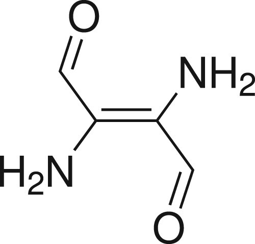
For our investigation, we limited ourselves to the so-called ‘H chromophore’ (Scheme 1), which has already been used in semiempirical studies by Lüttke et al. [78] and Dähne and Leupold [79], and was also considered by Serrano-Andrés and Roos [20]. Given a small basis set, this compound can be treated with highly correlated multireference methods using a reasonably large active space of six electrons in six active orbitals (CAS(6,6), including the full central π-system). We did not consider including the n-electrons in the active space since these do not contribute significantly to the ${\mathrm{S}}_0\to {\mathrm{S}}_1$ transition [20].

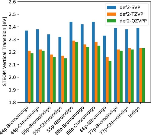
Figure 1. Vertical transition energies computed by the DLPNO-STEOM method for a set of symmetrically substituted indigo dyes. Data plotted from Table 2.

Scheme 1. Simplified central ‘H chromophore’ of indigo.

The computed energies for the S${}_0$ and S${}_1$ states can be found in Table 1. We should note that all multireference correlated methods, fully internally contracted (fic-)NEVPT2 (also called ‘partially contracted’) [80,81], uncontracted (uc-)MRCI, and fic-MRCC ([82], see Supplementary Material for details), use the same SA-CASSCF wave function averaged over the S${}_0$ and S${}_1$ states. Furthermore, all methods presented in Table 1 are truncated after doubles excitations. The fic-NEVPT2 results are comparable to previous reports [20] and match the results from a DLPNO-STEOM calculation very well. A higher energy difference is reported by the fic-MRCC and the single-reference EOMCC methods at about 3.5 eV and 3.4 eV, respectively, with the results from the uc-MRCI falling roughly between these and the STEOM results.

Table 1. Total energies for the ${\mathrm{S}}_0$ and ${\mathrm{S}}_1$ states of the H chromophore $({\text{E}}_{\mathrm{h}})$. The excitation energy to the S₁ state, ω, is computed in eV. Here, we understand ‘STEOM’ to mean ‘DLPNO-STEOM’ with identical settings as in the remaining calculations in this paper. All other methods are canonical.

	CASSCF	fic-NEVPT2	uc-MRCI	fic-MRCC	EOMCC	STEOM
S${}_0$	−413.304138	−414.457377	−414.457254	−414.507567	−414.492813	−414.492887
S${}_1$	−413.129797	−414.346606	−414.341664	−414.379725	−414.368914	−414.381096
ω	4.744	3.014	3.145	3.479	3.371	3.042

Table 2. Vertical transition energies computed by the DLPNO-STEOM method for a set of symmetrically substituted indigo dyes.

Compound	def2-SVP	def2-TZVP	def2-QZVPP
Indigo	2.39	2.23	2.23
4,4'-Bromoindigo	2.37	2.21	2.19
4,4'-Chloroindigo	2.38	2.22	2.21
5,5'-Bromoindigo	2.34	2.18	2.16
5,5'-Chloroindigo	2.32	2.17	2.15
5,5'-Nitroindigo	2.44	2.29	2.28
6,6'-Bromoindigo	2.42	2.26	2.24
6,6'-Chloroindigo	2.44	2.28	2.25
6,6'-Nitroindigo	2.33	2.16	2.13
7,7'-Bromoindigo	2.39	2.22	2.21
7,7'-Chloroindigo	2.38	2.23	2.22
Deviation from def2-QZVPP
Max(−)	0.16	0.00
ME	0.17	0.01
Max(+)	0.19	0.03
SD	0.01	0.01
MAE	0.17	0.01

All values are given in eV.

Thus, we conclude that a genuine multireference treatment is not required. This is mainly evidenced by the fact that, in the state-averaged multiconfigurational wave function, the S${}_0$ and S${}_1$ states are dominated ($\approx 90\mathrm{\%}$) by a single configuration, and the transition can be characterised as singles-dominated $\pi \to {\pi }^{\ast }$. This could also explain why the fic-MRCC and EOMCC results are rather close and the DLPNO-STEOM results are lower by $\sim 0.4\mathrm{eV}$: STEOM-CCSD contains an implicit triples term absent in both EOM-CCSD [29,30] and in fic-MRCCSD. Since the wave function is dominated by two configurations, implicit higher-order excitations do not play a significant role in the fic-MRCC results.

Furthermore, EOMCC methods can be used to treat multiconfigurational situations given that certain parameters are fulfilled. For EOM-CCSD, this usually means that the singles character is required to be greater than $\mathrm{\%}{T}_1>90\mathrm{\%}$, and in STEOM calculations the active space character should be $>95\mathrm{\%}$ [46,59]. Both criteria were fulfilled in our calculations.

4.2. Basis set effects

In accordance with our earlier experience [52], triple-ζ basis sets seem to be a good compromise between accuracy and efficiency when calculating the optical spectra of dyes. The Max(+) values in Table 2 are calculated using the def2-QZVPP values as reference and they indicate that the def2-SVP basis set does not produce converged results, with its Max(+) being $0.19\mathrm{eV}$. While these calculations are fast (about 20 min on 8 cores for Indigo) and yield a tolerable accuracy for some purposes, it is still above our target threshold of $0.1\mathrm{eV}$. The def2-TZVP values, on the other hand, deviates only up to $\mathrm{Max}(+)=0.03\mathrm{eV}$ and 0.01 eV on average from the def2-QZVPP results, which is not only well below the desired threshold but also still cheap. A def2-TZVP calculation on Indigo takes about 2 hours on 8 cores, while obtaining the slightly better def2-QZVPP values takes about 7.5 hours on 16 cores. Thus, the def2-TZVP basis set will be used in the remainder of this study for all geometry optimisations, STEOM and ESD calculations.

4.3. Solvent effects

As a last step before calculating the full benchmark set from Jacquemin et al. [13], the magnitude of the CPCM implicit solvation effects on the STEOM calculations will also be assessed. To this end, we selected a few symmetrically substituted indigo dyes from the full set, including Tyrian purple (6,6'-dibromoindigo), and optimised the geometries at the B3LYP-D3(BJ)-CPCM/def2-TZVP level of theory. Subsequently, we computed the DLPNO-STEOM vertical transition energies for each of the optimised geometries, again including solvation effects through CPCM. The results are presented in Table 3. As expected, the average effect grows as the relative permittivity increases and ranges between 0.09 eV and 0.16 eV. For the least polar solvents, CCl₄, Xylene and Benzene, the effect is about 0.10 eV, for the solvents of medium polarisation, CHCl₃ and TCE, it is about 0.135 eV, and for the most polar ones, ethanol and DMSO, the effect is about 0.155 eV. Table S2 of the Supplementary Material also indicates the magnitude of the indirect solvent effects that are due to solvating the molecular orbitals and the ground-state CC amplitudes. It turns out that on average 75% of the solvent shift is due to indirect effects and this ratio slightly increases with polarity. Nevertheless, the direct contributions from the STEOM step are not negligible. As also discussed by Jacquemin [13], the effects could be larger for polar solvents than the CPCM numbers indicate. This is especially true for ethanol, where the formation of hydrogen bonds introduces specific interactions that are not included in the CPCM model. Although we do not plan to account for such specific interactions in this study, the inclusion of solvent effects using CPCM is certainly necessary. All subsequent calculations contain the CPCM correction for the various solvents considered.

Table 3. Solvation effects compared to gas-phase STEOM calculations. Solvents sorted with increasing dielectric constant ε from left to right.

	CCl4	Xylene	Benzene	CHCl3	TCE	EtOH	DMSO
ε	2.24	2.27	2.28	4.9	8.2	24.3	47.2
Indigo	−0.099	−0.101	−0.101	−0.137	−0.153	−0.155	−0.164
4,4'-Bromoindigo	−0.100	−0.102	−0.102	−0.137	−0.156	−0.165	−0.173
4,4'-Chloroindigo	−0.102	−0.104	−0.104	−0.140	−0.155	−0.166	−0.175
5,5'-Bromoindigo	−0.093	−0.095	−0.095	−0.124	−0.138	−0.145	−0.153
5,5'-Chloroindigo	−0.096	−0.097	−0.098	−0.121	−0.135	−0.142	−0.150
5,5'-Nitroindigo	−0.082	−0.083	−0.075	−0.109	−0.123	−0.128	−0.138
6,6'-Bromoindigo	−0.100	−0.102	−0.103	−0.135	−0.151	−0.156	−0.168
6,6'-Chloroindigo	−0.102	−0.104	−0.104	−0.138	−0.153	−0.162	−0.170
6,6'-Nitroindigo	−0.106	−0.127	−0.127	−0.157	−0.175	−0.185	−0.195
7,7'-Bromoindigo	−0.078	−0.080	−0.081	−0.108	−0.120	−0.126	−0.134
7,7'-Chloroindigo	−0.087	−0.089	−0.089	−0.116	−0.132	−0.134	−0.142
Average	−0.095	−0.099	−0.098	−0.129	−0.145	−0.151	−0.160

All values are given in eV.

4.4. Benchmark results

The main results of our study are presented in Table 4. To facilitate comparison with experimental absorption band maxima, the CPCM-corrected DLPNO-STEOM values still need to be corrected for vibronic effects to arrive at a computational estimate of the 0–0 transition energy. At the VG level, this correction can be obtained from DFT frequencies and displacements. This is a relatively small correction: while the STEOM energies are all close to 2.0 eV within a few tenths of eVs, the VG shift, ${\omega }_{\mathrm{VG}}$, is typically $-0.05\mathrm{eV}$, see Table 5. Summing up these values yields the DLPNO-STEOM 0–0 energies, ${\omega }_{0-0}$, which can be compared to experiment.

Table 4. Benchmark results: the CPCM-corrected DLPNO-STEOM excitation energy (ω), the VG correction ${\omega }_{\mathrm{VG}}$, the 0–0 transition energy (${\omega }_{0-0}$), the experimental absorption band maxima (${\omega }_{\exp }$) [13] and the error of the total STEOM estimate with respect to experiment ($\mathrm{\Delta }\omega$).

Name	Solvent	ω	${\omega }_{\mathrm{VG}}$	${\omega }_{0-0}$	${\omega }_{exp}$	$\mathrm{\Delta }\omega$
Indigo	Benzene	2.13	−0.05	2.09	2.08	0.00
Indigo	CCl${}_4$	2.13	−0.05	2.09	2.09	0.00
Indigo	CHCl${}_3$	2.10	−0.05	2.05	2.05	0.00
Indigo	DMSO	2.07	−0.05	2.02	2.00	0.02
Indigo	EtOH	2.08	−0.05	2.03	2.04	−0.01
Indigo	TCE	2.08	−0.05	2.03	2.02	0.01
4-Bromoindigo	TCE	2.08	−0.05	2.03	2.03	−0.01
5-Bromoindigo	Benzene	2.12	−0.05	2.07	2.05	0.02
5-Bromoindigo	TCE	2.07	−0.05	2.02	2.02	0.00
6-Bromoindigo	TCE	2.08	−0.05	2.03	2.06	−0.03
7-Bromoindigo	TCE	2.08	−0.05	2.03	2.05	−0.02
4,4'-Bromoindigo	TCE	2.06	−0.05	2.00	2.03	−0.02
4,4'-Chloroindigo	CHCl${}_3$	2.08	−0.05	2.03	2.05	−0.02
4,4'-Chloroindigo	EtOH	2.06	−0.05	2.00	2.03	−0.02
4,4'-Chloroindigo	TCE	2.07	−0.05	2.01	2.02	−0.01
4,4'-Chloroindigo	Xylene	2.12	−0.05	2.07	2.07	0.00
4,4'-Methoxycarbonylindigo	EtOH	2.03	−0.05	1.98	2.03	−0.04
4,4'-Methoxyindigo	TCE	2.09	−0.06	2.03	2.06	−0.02
5,5'-Bromoindigo	CHCl${}_3$	2.06	−0.05	2.00	2.03	−0.03
5,5'-Bromoindigo	EtOH	2.03	−0.05	1.98	2.01	−0.03
5,5'-Bromoindigo	TCE	2.04	−0.05	1.99	2.00	−0.01
5,5'-Bromoindigo	Xylene	2.08	−0.05	2.03	2.05	−0.02
5,5'-Chloroindigo	EtOH	2.02	−0.05	1.97	2.02	−0.04
5,5'-Chloroindigo	TCE	2.03	−0.05	1.98	2.00	−0.02
5,5'-Chloroindigo	Xylene	2.07	−0.05	2.02	2.05	−0.03
5,5'-Fluoroindigo	CHCl${}_3$	2.02	−0.05	1.97	2.01	−0.04
5,5'-Fluoroindigo	TCE	2.01	−0.05	1.96	2.02	−0.06
5,5'-Methoxyindigo	TCE	1.90	−0.07	1.83	1.91	−0.08
5,5'-Methylindigo	CHCl${}_3$	2.04	−0.05	1.99	2.01	−0.02
5,5'-Methylindigo	TCE	2.03	−0.05	1.97	2.00	−0.03
5,5'-Nitroindigo	TCE	2.16	−0.05	2.11	2.14	−0.03
6,6'-Bromoindigo	TCE	2.11	−0.05	2.06	2.11	−0.05
6,6'-Bromoindigo	Xylene	2.16	−0.04	2.11	2.10	0.01
6,6'-Chloroindigo	EtOH	2.12	−0.05	2.07	2.18	−0.11
6,6'-Chloroindigo	TCE	2.13	−0.05	2.08	2.10	−0.02
6,6'-Chloroindigo	Xylene	2.18	−0.04	2.13	2.22	−0.08
6,6'-Fluoroindigo	TCE	2.20	−0.05	2.14	2.18	−0.03
6,6'-Methoxyindigo	TCE	2.24	−0.06	2.18	2.16	0.02
6,6'-Methylindigo	TCE	2.11	−0.05	2.06	2.08	−0.02
6,6'-Methylindigo	Xylene	2.15	−0.05	2.10	2.11	−0.01
6,6'-Nitroindigo	TCE	1.98	−0.05	1.93	1.95	−0.02
6,6'-Nitroindigo	Xylene	2.03	−0.04	1.99	1.96	0.03
7,7'-Bromoindigo	TCE	2.10	−0.06	2.05	2.05	0.00
7,7'-Chloroindigo	EtOH	2.09	−0.06	2.04	2.10	−0.07
7,7'-Chloroindigo	TCE	2.09	−0.06	2.04	2.06	−0.02
7,7'-Fluoroindigo	CHCl${}_3$	2.09	−0.05	2.04	2.00	0.03
7,7'-Fluoroindigo	TCE	2.08	−0.06	2.02	2.05	−0.03
7,7'-Methoxyindigo	TCE	1.97	−0.08	1.89	1.93	−0.03
7,7'-Methylindigo	CHCl${}_3$	2.08	−0.06	2.02	2.03	−0.01
7,7'-Methylindigo	Xylene	2.11	−0.06	2.06	2.05	0.00
5,5',7-Bromoindigo	Xylene	2.09	−0.05	2.04	2.03	0.01
4,4',5,5'-Bromoindigo	Benzene	2.07	−0.05	2.02	2.02	0.00
4,4',5,5'-Chloroindigo	TCE	2.03	−0.05	1.98	1.99	−0.01
4,4',6,6'-Chloroindigo	TCE	2.09	−0.05	2.04	2.08	−0.04
4,4',6,6'-Methylindigo	Xylene	2.13	−0.05	2.08	2.09	0.00
4,4',7,7'-Chloroindigo	TCE	2.06	−0.06	2.01	2.03	−0.03
4,4',7,7'-Chloroindigo	Xylene	2.11	–0.05	2.05	2.08	−0.02
4,4',7,7'-Methylindigo	Xylene	2.07	−0.06	2.01	2.06	−0.05
5,5',6,6'-Chloroindigo	TCE	2.05	−0.05	2.00	2.05	−0.05
5,5',6,6'-Methylindigo	Xylene	2.10	−0.05	2.04	2.05	−0.01
5,5',7,7'-Bromoindigo	Benzene	2.08	−0.06	2.03	2.02	0.01
5,5',7,7'-Bromoindigo	CHCl${}_3$	2.06	−0.06	2.00	2.02	−0.01
5,5',7,7'-Bromoindigo	EtOH	2.04	−0.06	1.98	2.00	−0.02
5,5',7,7'-Bromoindigo	TCE	2.05	−0.06	1.99	2.00	0.00
5,5',7,7'-Bromoindigo	Xylene	2.08	−0.06	2.03	2.02	0.00
5,5',7,7'-Chloroindigo	EtOH	2.03	−0.06	1.97	2.02	−0.04
5,5',7,7'-Chloroindigo	TCE	2.04	−0.06	1.98	2.00	−0.02
5,5',7,7'-Chloroindigo	Xylene	2.07	−0.06	2.01	2.03	−0.02
6,6',7,7'-Chloroindigo	TCE	2.12	−0.05	2.07	2.10	−0.03
6,6',7,7'-Methylindigo	Xylene	2.08	−0.05	2.03	2.08	−0.06
4,4'-Chloro-5,5'-bromoindigo	CHCl${}_3$	2.04	−0.05	1.99	2.03	−0.04
4,4'-Chloro-5,5'-bromoindigo	TCE	2.02	−0.05	1.97	2.00	−0.03
4,4'-Chloro-5,5'-bromoindigo	Xylene	2.07	−0.05	2.02	2.02	0.00
5,5'-Chloro-7,7'-bromoindigo	Xylene	2.07	−0.06	2.02	2.03	−0.01
4,4',5,5',6,6'-Chloroindigo	TCE	2.03	−0.05	1.98	2.03	−0.05
4,4',5,5',7,7'-Bromoindigo	CHCl${}_3$	2.03	−0.06	1.98	1.99	−0.01
4,4',5,5',7,7'-Bromoindigo	Xylene	2.05	−0.05	1.99	2.01	−0.02
4,4',5,5',7,7'-Chloroindigo	TCE	2.03	−0.06	1.98	2.02	−0.04
4,4',5,5',7,7'-Chloroindigo	Xylene	2.07	−0.05	2.02	2.02	−0.01
4,4',6,6',7,7'-Chloroindigo	TCE	2.09	−0.05	2.03	2.08	−0.05
5,5',6,6',7,7'-Chloroindigo	TCE	2.05	−0.05	2.00	2.07	−0.07
5,5',7,7'-Bromo-6,6'-aminoindigo	Xylene	2.31	−0.07	2.25	2.22	0.03
4,4',5,5',6,6',7,7'-Chloroindigo	EtOH	2.03	−0.05	1.98	2.05	−0.07
4,4',5,5',6,6',7,7'-Chloroindigo	TCE	2.04	−0.05	1.98	2.02	−0.04
4,4',5,5',6,6',7,7'-Chloroindigo	Xylene	2.06	−0.05	2.01	2.04	−0.03

All values reported in eV.

Table 5. Statistical evaluation of the VG corrections (${\omega }_{\mathrm{VG}}$) and the errors in DLPNO-STEOM 0–0 transition energies (${\omega }_{0-0}$) from Table 4 with respect to the experimental values (eV).

	${{\omega }_{\mathrm{VG}}}^{†}$	${\omega }_{0-0}$
Max(−)	−0.08	−0.11
ME	−0.05	−0.02
Max(+)	−0.04	0.03
SD	0.01	0.03
MAE	0.05	0.03

${}^{†}$ For ${\omega }_{\mathrm{VG}}$, the smallest, average, maximum, … shifts are reported instead of errors.

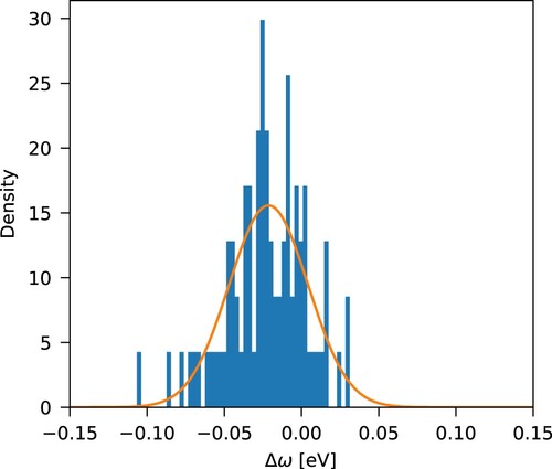
The deviations between predicted and experimental values ($\mathrm{\Delta }\omega$; averaged experimental values computed by Jacquemin et al. [13]; for individual measurements see references therein) are presented in Table 4 as well as in Figure 2, while the statistics can be found in Table 5. On average, the STEOM error is $-0.02\mathrm{eV}$ for this family of dyes, the maximum deviation being $-0.11\mathrm{eV}$. This indicates that in general, the computed values are lower than the measured ones. The deviation from experiment tends to be larger for polar solvents, as expected. Nevertheless, even for the most polar EtOH and DMSO solvents, the average deviation from experiment is only $-0.04\mathrm{eV}$. The protocol we present here consists of many components including the DLPNO-STEOM vertical excitation energies, the CPCM correction calculated from STEOM amplitudes using the CIS formula and the VG shift obtained at the DFT level. The performance of these have been evaluated independently, to the extent this is possible. Thus, the eventual excellent agreement between the predicted and measured 0–0 transitions indicates the reliability of the proposed protocol and it certainly agrees with our initial goal of providing an affordable computational method that delivers excitation energies within 0.1 eV for a large number of chemically relevant molecules.

Figure 2. Normalized error density distribution with respect to experiment, $\mathrm{\Delta }\omega$, from Table 4, with a Gaussian probability density function overlaid.

4.5. Chemical substitution

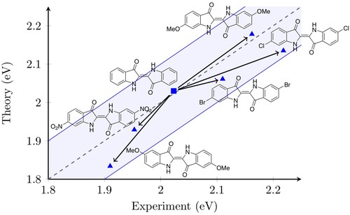
As a further illustration, we now turn to investigating the effect of chemical substitutions on the CPCM-corrected DLPNO-STEOM 0–0 transition energy. Figure 3 shows how the excitation energy of indigo changes as various substituents are added to the core structure. Indigo in TCE is one of the few dyes for which our protocol predicts a slightly too high value. Most derivatives lie in the band stretching between perfect agreement and $-0.1\mathrm{eV}$ deviation from experiment. Among these is 6,6'-dibromoindigo in TCE. It is interesting to note that the shift caused by the Br substituents is relatively small compared especially to the methoxy and Cl substituents at the same position. In fact, 6,6'-dichloroindigo is the only dye in Figure 3 that is dissolved in Xylene and is shown mainly because it features the largest measured positive shift compared to indigo. The STEOM error for 6,6'-dichloroindigo is also quite large in Xylene ($-0.08\mathrm{eV}$), and it is the largest in the test set when EtOH is used as the solvent ($-0.11\mathrm{eV}$). The methoxy groups are notable because they are responsible both for some of the largest positive and negative shifts. In the 6,6' positions, these substituents cause a measured positive shift of about $0.14\mathrm{eV}$ with respect to the experimental absorption maximum of indigo at $2.02\mathrm{eV}$, while in the 5,5' positions they are responsible for a $-0.11\mathrm{eV}$ shift. By contrast, two nitro groups in the 6,6' positions cause only a $-0.07\mathrm{eV}$ shift. Nevertheless, for all these different substituents, our protocol remains within the $0.1\mathrm{eV}$ error bar and as a consequence, it is perfectly suitable for predicting the effects of chemical changes.

Figure 3. The effect of chemical substitutions on excitation energies. The dashed line indicates perfect agreement between theory and experiment, the shaded zone signifies the region within which the agreement is within ±0.1 eV.

4.6. Absorption spectra

Finally, the protocol under discussion allows for the calculation of entire absorption spectra. As an illustration, Figure 4 shows the computed and measured spectra of indigo, 6-bromoindigo and 6,6'-dibromoindigo in DMSO. The spectra predicted by our protocol agree remarkably well with the measured ones without any empirical shift. The only empirical parameter in the three computed spectra is the linewidth that was determined as a common parameter for all three of them from the half width at half maximum of the low-energy side of the experimental curves. This was done to avoid the broadening of the spectra due to a shoulder on the high-energy side. The stick plots below the computed curves indicate the contributions of vibrational modes. The highest peak at $\sim 16,000{\mathrm{cm}}^{-1}$ corresponds to the 0–0 transition, since at 0 K this is the lowest energy transition. As the spectra in Figure 4 are computed at room temperature, transitions from a vibrationally excited ground state (hot bands) can also just be observed at energies lower than the 0–0 transition. The shoulder towards higher energies ($\sim 18,000{\mathrm{cm}}^{-1}$) is mainly due to two similar fundamental modes that feature a strong symmetric stretching motion of the CC and CO bonds in the central chromophore, while the remaining system also participates in a symmetric stretching/rocking motion (the xyz trajectories are included in the Supplementary Material). Vibrational overtones are present in the computed spectra at even higher energies, although their intensity is extremely low. For a more detailed discussion of the vibrational progression and temperature effects, we refer to Section 2.3 and to the Supplementary Material, Section S5.

Figure 4. Normalized VIS absorption spectra for indigo, 6-bromoindigo, and 6,6'-dibromoindigo in DMSO. The unshifted computed spectra are presented with an inhomogeneous line width of $700{\mathrm{cm}}^{-1}$ as well as sticks for each vibrational mode. The experimental spectra were obtained from Ref. [83].

As a final touch, we also measured the absorption spectrum of a commercially available Tyrian purple dye in chloroform. The natural dye is a mixture of different isatinoids, indigoids, and indirubinoids [83], whose composition may naturally vary between different batches and types of shellfish used in the production process. Based on our results, the shoulder in Figure 5 at about $\sim 16500{\mathrm{cm}}^{-1}$ can be assigned to the indigoids, for which we indicated the 0–0 transitions (see Figure S3 of the Supplementary Material for measured and computed spectra of indigo in chloroform). Based on the spectral data from Ref. [83], the highest peak in Figure 5 corresponds to the region where the indirubinoids absorb visible light. Note that the isatinoids do not absorb in the energy range shown in Figure 5. Thus, to reproduce the full spectrum of this particular mixture, the spectra of the indirubinoids would also need to be calculated and the concentrations of the components would also need to be known. While this is out of the scope of the present study, we feel that the accuracy of our method has been demonstrated and its practical utility is well illustrated by our contribution to the study of indigoids in general and Tyrian purple in particular.

Figure 5. The spectrum of Tyrian purple and the 0–0 transition energies of three of its components studied in this paper. The shaded area corresponds to the region where indirubin dyes absorb (its width chosen from the spread between the band maxima of indigorubin dyes in Ref. [83] with an additional $500{\mathrm{cm}}^{-1}$ in both directions).

5. Conclusions

In our contribution to the Special Issue celebrating the scientific achievements of John Stanton, we have carried out an excited state coupled cluster study of indigoid dyes. After discussing the significance of these dyes, the DLPNO-STEOM method was introduced, and the perturbation theory of vibronic interactions was briefly discussed. Next, we investigated multireference effects and found that a single-reference method, such as ours, should be sufficient to provide accurate results for this family of dyes. After studying basis set effects, the def2-TZVP basis set was chosen as an excellent compromise between accuracy and efficiency. Implicit solvent effects also had to be taken into account in order to achieve our target accuracy of $0.1\mathrm{eV}$. We then presented our DLPNO-STEOM results for 0–0 transition energies and compared them to experimental absorption band maxima. We found that in virtually all cases, our predictions agree with experiment within $0.1\mathrm{eV}$ and that STEOM also reproduces the effects of chemical substitutions on the excitation energy. Finally, we presented our calculated spectra for some of the main components of Tyrian purple and also compared these findings to a measured spectrum of the same dye. It is especially important to emphasise that our protocol was able to reproduce the experimental spectra of individual components without any empirical shift. Thus, we are confident that the VG-corrected DLPNO-STEOM method will become a useful tool for computational chemists studying photochemical processes.

Acknowledgments

The authors thank Romain Berraud-Pache for acquiring the experimental spectra and for constructive discussions regarding the computational procedure.

Disclosure statement

No potential conflict of interest was reported by the author(s).

Correction Statement

This article has been republished with minor changes. These changes do not impact the academic content of the article.

Additional information

Funding

The authors thank the Max-Planck-Gesellschaft for financial support. R.I. thanks Middlebury College for financial support. M.H.L. gratefully acknowledges funding by the Studienstiftung des Deutschen Volkes and Verband der Chemischen Industrie.

References

- J. Hudson, The History of Chemistry, 1st ed. (Macmillan, London, 1992).
- K.St. Clair, The Secret Lives of Colors, 1st ed. (Penguin Books, New York, 2017).
- J. Balfour-Paul, Indigo: From Mummies to Blue Jeans, rev. edition ed. (British Museum Press, London, 2011).
- C.J. Cooksey, Molecules 6 (9), 736–769 (2001). doi:10.3390/60900736
- C. Cooksey, Sci. Prog. 96 (2), 171–186 (2013). doi:10.3184/003685013X13680345111425
- E.S.B. Ferreira, A.N. Hulme, H. McNab and A. Quye, Chem. Soc. Rev. 33, 329–336 (2004). doi:10.1039/b305697j
- E.D. Głowacki, G. Voss, L. Leonat, M. Irimia-Vladu, S. Bauer and N.S. Sariciftci, Isr. J. Chem. 52 (6), 540–551 (2012). doi:10.1002/ijch.201100130
- P.C. Ray, History of Chemistry in Ancient and Medieval India, 1st ed. (Indian Chemical Society, Calcutta, 1956).
- A. Baeyer, Ber. Dtsch. Chem. Ges. 16 (2), 2188–2204 (1883). doi:10.1002/cber.188301602130
- P. Friedländer, Ber. Dtsch. Chem. Ges 42 (1), 765–770 (1909). doi:10.1002/cber.190904201122
- M. Klessinger and W. Lüttke, Tetrahedron 19, 315–335 (1963). doi:10.1016/S0040-4020(63)80023-X
- H. Hermann and W. Lüttke, Chem. Ber 101 (5), 1708–1714 (1968). doi:10.1002/cber.19681010523
- D. Jacquemin, J. Preat, V. Wathelet and E.A. Perpète, J. Chem. Phys. 124 (7), 074104 (2006). doi:10.1063/1.2166018
- M. Moreno, J.M. Ortiz-Sánchez, R. Gelabert and J.M. Lluch, Phys. Chem. Chem. Phys. 15, 20236–20246 (2013). doi:10.1039/c3cp52763h
- Z. Ju, J. Sun and Y. Liu, Molecules 24 (21), 3831 (2019). doi:10.3390/molecules24213831.
- F. Cervantes-Navarro and D. Glossman-Mitnik, J. Photochem. Photobiol. A 255, 24–26 (2013). doi:10.1016/j.jphotochem.2013.01.011
- S. Shityakov, N. Roewer, C. Förster and J.A. Broscheit, Nanoscale Res. Lett. 12 (1), 439 (2017). doi:10.1186/s11671-017-2193-7
- J. Pina, D. Sarmento, M. Accoto, P.L. Gentili, L. Vaccaro, A. Galvão and J.S. Seixas de Melo, J. Phys. Chem. B 121 (10), 2308–2318 (2017). doi:10.1021/acs.jpcb.6b11020
- V. Barone, M. Biczysko, C. Latouche and A. Pasti, Theor. Chem. Acc 134 (12), 145 (2015). doi:10.1007/s00214-015-1753-0
- L. Serrano-Andrés and B.O. Roos, Chem. Eur. J. 3 (5), 717–725 (1997). doi:10.1002/chem.19970030511
- S. Yamazaki, A.L. Sobolewski and W. Domcke, Phys. Chem. Chem. Phys. 13, 1618–1628 (2011). doi:10.1039/C0CP01901A
- K. Emrich, Nucl. Phys. A 351 (3), 379–396 (1981). doi:10.1016/0375-9474(81)90179-2
- J.F. Stanton and R.J. Bartlett, J. Chem. Phys. 98 (9), 7029–7039 (1993). doi:10.1063/1.464746
- O. Christiansen, H. Koch and P. Jørgensen, Chem. Phys. Lett. 243 (5), 409–418 (1995). doi:10.1016/0009-2614(95)00841-Q
- J. Schirmer, Phys. Rev. A 26, 2395–2416 (1982). doi:10.1103/PhysRevA.26.2395
- A.B. Trofimov and J. Schirmer, J. Phys. B: At. Mol. Opt. Phys. 28 (12), 2299–2324 (1995). doi:10.1088/0953-4075/28/12/003
- J.F. Stanton and J. Gauss, J. Chem. Phys. 103 (3), 1064–1076 (1995). doi:10.1063/1.469817
- M. Nooijen and J.G. Snijders, J. Chem. Phys. 102 (4), 1681–1688 (1995). doi:10.1063/1.468900
- M. Nooijen and R.J. Bartlett, J. Chem. Phys. 107 (17), 6812–6830 (1997). doi:10.1063/1.474922
- M. Nooijen, Spectrochim. Acta A 55 (3), 539–559 (1999). doi:10.1016/S1386-1425(98)00261-3
- C. Riplinger and F. Neese, J. Chem. Phys. 138 (3), 034106 (2013). doi:10.1063/1.4773581
- P. Pinski, C. Riplinger, E.F. Valeev and F. Neese, J. Chem. Phys. 143 (3), 034108 (2015). doi:10.1063/1.4926879
- C. Riplinger, P. Pinski, U. Becker, E.F. Valeev and F. Neese, J. Chem. Phys. 144 (2), 024109 (2016). doi:10.1063/1.4939030
- W. Kutzelnigg, Theor. Chim. Acta. 1 (4), 327–342 (1963). doi:10.1007/BF00528764
- B. Helmich and C. Hättig, J. Chem. Phys. 135 (21), 214106 (2011). doi:10.1063/1.3664902
- M.S. Frank and C. Hättig, J. Chem. Phys. 148 (13), 134102 (2018). doi:10.1063/1.5018514
- C. Peng, M.C. Clement and E.F. Valeev, J. Chem. Theory Comput. 14 (11), 5597–5607 (2018). doi:10.1021/acs.jctc.8b00171
- A.K. Dutta, M. Saitow, C. Riplinger, F. Neese and R. Izsák, J. Chem. Phys. 148 (24), 244101 (2018). doi:10.1063/1.5029470
- S. Haldar, C. Riplinger, B. Demoulin, F. Neese, R. Izsak and A.K. Dutta, J. Chem. Theory Comput.15 (4), 2265–2277 (2019). doi:10.1021/acs.jctc.8b01263
- A.K. Dutta, M. Saitow, B. Demoulin, F. Neese and R. Izsák, J. Chem. Phys. 150 (16), 164123 (2019). doi:10.1063/1.5089637
- S. Haldar and A.K. Dutta, J. Phys. Chem. A 124 (19), 3947–3962 (2020). doi:10.1021/acs.jpca.0c01793
- A.K. Dutta, F. Neese and R. Izsák, J. Chem. Phys. 145 (3), 034102 (2016). doi:10.1063/1.4958734
- M. Nooijen and J.G. Snijders, Int. J. Quantum Chem. 48 (1), 15–48 (1993). doi:10.1002/qua.560480103
- J.F. Stanton and J. Gauss, J. Chem. Phys. 101 (10), 8938–8944 (1994). doi:10.1063/1.468022
- M. Nooijen and R.J. Bartlett, J. Chem. Phys. 102 (9), 3629–3647 (1995). doi:10.1063/1.468592
- A.K. Dutta, M. Nooijen, F. Neese and R. Izsák, J. Chem. Theory Comput. 14 (1), 72–91 (2018). doi:10.1021/acs.jctc.7b00802
- C.E. Schulz, A.K. Dutta, R. Izsák and D.A. Pantazis, J. Comput. Chem. 39 (29), 2439–2451 (2018). doi:10.1002/jcc.v39.29
- A. Dittmer, R. Izsák, F. Neese and D. Maganas, Inorg. Chem. 58 (14), 9303–9315 (2019). doi:10.1021/acs.inorgchem.9b00994
- R. Berraud-Pache, F. Neese, G. Bistoni and R. Izsák, J. Phys. Chem. Lett. 10 (17), 4822–4828 (2019). doi:10.1021/acs.jpclett.9b02240
- A. Sirohiwal, R. Berraud-Pache, F. Neese, R. Izsák and D.A. Pantazis, J. Phys. Chem. B 124 (40), 8761–8771 (2020). doi:10.1021/acs.jpcb.0c05761
- R. Berraud-Pache, E. Santamaría-Aranda, B. de Souza, G. Bistoni, F. Neese, D. Sampedro and R. Izsák, Chem. Sci. 12, 2916–2924 (2021). doi:10.1039/D0SC06575G
- R. Berraud-Pache, F. Neese, G. Bistoni and R. Izsák, J. Chem. Theory Comput. 16 (1), 564–575 (2020). doi:10.1021/acs.jctc.9b00559
- A. Sirohiwal, F. Neese and D.A. Pantazis, J. Am. Chem. Soc. 142 (42), 18174–18190 (2020). doi:10.1021/jacs.0c08526
- A. Sirohiwal, F. Neese and D.A. Pantazis, J. Chem. Theory Comput. 17 (3), 1858–1873 (2021). doi:10.1021/acs.jctc.0c01152
- B. de Souza, F. Neese and R. Izsák, J. Chem. Phys. 148 (3), 034104 (2018). doi:10.1063/1.5010895
- R. Izsák, Wiley Interdiscip. Rev. Comput. Mol. Sci. 10 (3), e1445 (2020). doi:10.1002/wcms.1445
- R. Izsák, Int. J. Quantum Chem. 121 (3), e26327 (2021). doi:10.1002/qua.26327
- J.F. Stanton, Faraday Discuss. 150, 331–343 (2011). doi:10.1039/c0fd00029a
- A.K. Dutta, M. Nooijen, F. Neese and R. Izsák, J. Chem. Phys 146 (7), 074103 (2017). doi:10.1063/1.4976130
- S.F. Boys, Rev. Mod. Phys. 32, 296–299 (1960). doi:10.1103/RevModPhys.32.296
- J. Pipek and P.G. Mezey, J. Chem. Phys. 90 (9), 4916–4926 (1989). doi:10.1063/1.456588
- P. Pulay, Chem. Phys. Lett. 100 (2), 151–154 (1983). doi:10.1016/0009-2614(83)80703-9
- O. Vahtras, J. Almlöf and M. Feyereisen, Chem. Phys. Lett. 213 (5), 514–518 (1993). doi:10.1016/0009-2614(93)89151-7
- K. Eichkorn, O. Treutler, H. Öhm, M. Häser and R. Ahlrichs, Chem. Phys. Lett. 242 (6), 652–660 (1995). doi:10.1016/0009-2614(95)00838-U
- D.G. Liakos, M. Sparta, M.K. Kesharwani, J.M.L. Martin and F. Neese, J. Chem. Theory Comput.11 (4), 1525–1539 (2015). doi:10.1021/ct501129s
- S. Ghosh, A.K. Dutta, B. de Souza, R. Berraud-Pache and R. Izsák, Mol. Phys. 118 (19–20), e1818858 (2020). doi:10.1080/00268976.2020.1818858
- V. Barone and M. Cossi, J. Phys. Chem. A 102 (11), 1995–2001 (1998). doi:10.1021/jp9716997
- Y. Niu, Q. Peng, C. Deng, X. Gao and Z. Shuai, J. Phys. Chem. A 114 (30), 7817–7831 (2010). doi:10.1021/jp101568f
- A. Baiardi, J. Bloino and V. Barone, J. Chem. Theory Comput 9 (9), 4097–4115 (2013). doi:10.1021/ct400450k
- F.J. Avila Ferrer and F. Santoro, Phys. Chem. Chem. Phys. 14, 13549–13563 (2012). doi:10.1039/c2cp41169e
- F. Neese, Wiley Interdiscip. Rev. Comput. Mol. Sci 8 (1), e1327 (2018). doi:10.1002/wcms.2018.8.issue-1
- P.J. Stephens, F.J. Devlin, C.F. Chabalowski and M.J. Frisch, J. Phys. Chem 98 (45), 11623–11627 (1994). doi:10.1021/j100096a001
- F. Weigend and R. Ahlrichs, Phys. Chem. Chem. Phys 7 (18), 3297–3305 (2005). doi:10.1039/b508541a
- F. Weigend, Phys. Chem. Chem. Phys. 8 (9), 1057–1065 (2006). doi:10.1039/b515623h
- S. Grimme, J. Antony, S. Ehrlich and H. Krieg, J. Chem. Phys. 132 (15), 154104 (2010). doi:10.1063/1.3382344
- F. Neese, F. Wennmohs, A. Hansen and U. Becker, Chem. Phys. 356 (1–3), 98–109 (2009). doi:10.1016/j.chemphys.2008.10.036
- R. Izsák and F. Neese, J. Chem. Phys 135 (14), 144105 (2011). doi:10.1063/1.3646921
- W. Lüttke, H. Hermann and M. Klessinger, Angew. Chem. Int. Ed 5 (6), 598–599 (1966). doi:10.1002/anie.196605982
- S. Dähne and D. Leupold, Angew. Chem. Int. Ed 5 (12), 984–993 (1966). doi:10.1002/anie.196609841
- C. Angeli, R. Cimiraglia, S. Evangelisti, T. Leininger and J.P. Malrieu, J. Chem. Phys 114 (23), 10252–10264 (2001). doi:10.1063/1.1361246
- C. Angeli, R. Cimiraglia and J.P. Malrieu, J. Chem. Phys 117 (20), 9138–9153 (2002). doi:10.1063/1.1515317
- M.H. Lechner, A. Papadopoulos, K. Sivalingam, A. Koslowski, A.A. Auer, U. Becker, F. Wennmohs and F. Neese, J. Comput. Chem. (to be published).
- Z.C. Koren, in Indirubin, the Red Shade of Indigo, edited by L. Meijer, N. Guyard, L. Skalsounis and G. Eisenbrand, Chap. 5 (Ed. ‘Life in Progress’, Roscoff, France, 2006).