Precise measurement of the D₂ S₁(0) vibrational transition frequency

Abstract

We report the absolute frequency of the $v^{\prime }=1,N^{\prime }=2\leftarrow v^{″}=0,N^{″}=0$ vibrational transition in the $X{}^1{\mathrm{\Sigma }}^{+}$ electronic ground state of D${}_2$. Deuterium molecules in the $v^{″}=0,N^{″}=0$ state in a molecular beam are excited to $v^{\prime }=1,N^{\prime }=2$ using a narrow-linewidth continuous-wave laser stabilised to an optical frequency comb; a strong static electric field in the excitation region induces a transition dipole moment, greatly enhancing the transition strength. Molecules excited to $v^{\prime }=1,N^{\prime }=2$ are state-selectively ionised using a pulsed ultraviolet laser and mass-selectively detected. Spectra recorded by scanning the infrared laser frequency are fit with a multi-Gaussian model that accounts for the intensities and relative frequencies of all hyperfine components at the static electric field strength used in the measurement. Zero-field absolute transition frequencies were determined from fits of 28 spectra recorded at nine different field strengths. Statistical uncertainty and systematic uncertainties due to the field plate spacing and relative intensities of the hyperfine components comprise the bulk of the overall uncertainty. We determine an absolute S${}_1$(0) transition frequency of 94,925,100,487(17) kHz after correcting for the photon recoil and second-order Doppler shifts. This value agrees with other recent experimental measurements and a theoretical prediction, but with a lower fractional uncertainty of only 0.2 ppb.

GRAPHICAL ABSTRACT

Keywords:

• Precision spectroscopy
• vibrational spectroscopy
• molecular hydrogen
• optical frequency comb
• molecular beam

1. Introduction

Precise measurements of the vibrational transition frequencies of the isotopologues of molecular hydrogen provide a means to test fundamental physics. Because these frequencies can be predicted with high precision using ab-initio theory, comparisons between theory and experiment can be used to search for new fundamental forces not predicted by the standard model, test quantum electrodynamics, and provide improved estimates of the nucleon-electron mass ratios [1,2]. Currently, predictions of the vibrational transition frequencies are available for all isotopologues with reported relative uncertainties of 4–5 parts per billion (ppb, ${10}^{-9}$) [1], and fourteen independent transition frequency measurements have been reported with uncertainties lower than the theoretical predictions [3–13]. Of these fourteen measurements, the six most precise are on the heteronuclear isotopologue, HD [6,7,9,10,13], and the most precise measurement on a homonuclear isotopologue [8] has a relative uncertainty nine times larger than the most precise measurement on HD [9]. This disparity can be attributed to the relative strength of the available transitions: while HD has weak dipole-allowed vibrational transitions, such transitions are forbidden in the homonuclear isotopologues due to the lack of a dipole moment and ortho/para selection rules, so most precise measurements of vibrational transition frequencies in the homonuclear isotopologues have instead relied on the weaker quadrupole transition moments.

In this work, we use a strong static electric field (up to ${10}^7\mathrm{V}/\mathrm{m}$) to induce a transition dipole moment in D${}_2$ molecules. At the maximum field strength achievable with our apparatus, the strength of the S${}_1$(0) transition ($v^{\prime }=1,N^{\prime }=2\leftarrow v^{″}=0,N^{″}=0$) in the $X{}^1{\mathrm{\Sigma }}^{+}$ electronic ground state is enhanced by a factor of nine over the quadrupole transition. While a similar approach has previously been used to record direct absorption spectra of hydrogen molecules in a gas cell [14–19], in the current work, we use a narrow-linewidth laser to excite D${}_2$ molecules in a supersonic molecular beam from the rovibronic ground state ($X{}^1{\mathrm{\Sigma }}^{+},v^{″}=0,N^{″}=0$) to the $v^{\prime }=1,N^{\prime }=2$ excited state. The vibrational excitation efficiency is then measured using state-selective resonance-enhanced multiphoton ionisation (REMPI) of the $v^{\prime }=1,N^{\prime }=2$ state through the $EF{}^1{\mathrm{\Sigma }}^{+},v=0,N=2$ intermediate state. Spectra are recorded by scanning the infrared laser and measuring the ion intensity in the 4 amu channel using a time-of-flight mass spectrometer. Based on these spectra, we are able to determine the absolute transition frequency of the S${}_1$(0) transition with an uncertainty of 17 kHz or 0.2 ppb fractional uncertainty.

2. Experimental setup

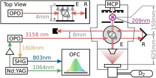
The experimental setup used for these measurements consists of a precision laser system that produces a narrow-linewidth, continuous-wave beam near 3158 nm with a well-defined and tunable absolute frequency and a molecular beam apparatus for producing a cold collimated beam of isolated deuterium molecules. The laser system has been described in a previous work [10]. In short: a 1064-nm reference laser is stabilised at an optical frequency of ${\nu }_{1064}=\mathrm{281,630,101.7}\mathrm{MHz}$ by frequency doubling the laser to $2{\nu }_{1064}=\mathrm{563,260,203.4}\mathrm{MHz}$ using second-harmonic generation and interrogating the $a_{10}$ component of the R(56) 32–0 transition of molecular iodine. The two degrees of freedom of a Ti:Sapphire-based optical frequency comb are stabilised so that mode number $n_{1064}=\mathrm{281,629}$ is 100 MHz lower in frequency than ${\nu }_{1064}$ and mode number $2n_{1064}$ is 200 MHz lower in frequency than $2{\nu }_{1064}$. This scheme results in a carrier-envelope offset frequency of $f_0=0$ and a repetition rate of $f_r=({\nu }_{1064}-100\mathrm{MHz})/n_{1064}\approx \mathrm{1,000,003,556.8}\mathrm{Hz}$. The exact value of $f_r$ during the measurement is recorded using a radio-frequency counter referenced to a rubidium oscillator which is disciplined by a global navigation satellite system (GNSS) receiver. Part of the 1064-nm beam is amplified to ∼10 W and used to pump a continuous-wave optical parametric oscillator (OPO), which down converts the pump photons into signal and idler photons at 1606 nm and 3158 nm, respectively. The signal beam is frequency doubled to 803 nm, and the frequency of the doubled beam is measured relative to mode $n_{2s}=\mathrm{373,409}$ of the optical frequency comb using a beat note detector. A phase-locked loop acting on a piezo mirror in the OPO cavity maintains the beatnote at a frequency $f_{\mathrm{bn},2s}$, which is defined using a tunable radio-frequency reference. The ∼2-W idler beam, with an absolute frequency given by (1) ${\nu }_i=(n_{1064}-n_{2s}/2)f_r+100\mathrm{MHz}-f_{\mathrm{bn},2s}/2,$(1) is used to excite the D${}_2$ S${}_1$(0) vibrational transition.

Figure 1 shows a diagram of the molecular beam apparatus. Pure deuterium gas at a pressure of 5 bar absolute is expanded through the nozzle of a piezo-actuated pulsed valve into a high vacuum chamber at a repetition rate of 50 Hz, producing a beam of D${}_2$ molecules directed upward with an average forward velocity of approximately 2100 m/s. Approximately 625 mm from the nozzle, the molecules pass between two 35-mm diameter plates spaced approximately 4 mm apart. Potentials of up to ±20 kV can be applied to the plates, resulting in electric fields of up to ${10}^7\mathrm{V}/\mathrm{m}$ in the gap. The 4-mm $1/e^2$-diameter infrared spectroscopy laser passes through the gap between the plates, approximately perpendicular to the molecular beam. After exiting the chamber, the laser is retroreflected using a hollow corner cube retroreflector, resulting in a second beam antiparallel to the first and offset upward by 8 mm which also passes between the plates. The two laser beams are aligned $\sim {0.2}^{\circ }$ from perpendicular with the molecular beam so that the Doppler shift from the forward velocity of the molecular beam results in separate spectral peaks for the outgoing and returning laser beams. After passing through the infrared beams, the molecules travel an additional 150 mm to the entrance of a time-of-flight mass spectrometer where molecules in the $v^{\prime }=1,N^{\prime }=2$ state are first excited to the $EF{}^1{\mathrm{\Sigma }}^{+},v=0,N=2$ state with two photons from a 209-nm ns pulsed laser and subsequently ionised with one more photon from the same laser. The 209-nm laser pulse is produced using third harmonic generation of a 627-nm dye laser pumped by a Nd:YAG laser at 532 nm. An electric field generated by two plates around the ionisation position (∼9 mm apart) accelerates the D${}_2^{+}$ ions upward into a field-free region and toward a microchannel plate detector, where their arrival time distribution is recorded with a digitising oscilloscope.

Figure 1. Schematic diagram of the experimental apparatus. The right section shows the molecular beam apparatus. D${}_2$ gas is expanded through the nozzle of a pulsed valve. The molecules travel upward and pass between two parallel field plates, where they are excited by the counterpropagating beams of the infrared spectroscopy laser. The outgoing beam is retroreflected using a corner cube retroreflector to produce a second, anti-parallel beam 8 mm above the first. A top view of the field plates and infrared beams is shown in the upper left corner. Approximately 150 mm further downstream, molecules in the $v^{\prime }=1,N^{\prime }=2$ vibrational excited state are state-selectively ionised using a pulsed UV laser and mass-selectively detected using a time-of-flight mass spectrometer. The infrared spectroscopy laser is the idler of an OPO, and its absolute frequency is stabilised by comparing the pump and frequency-doubled signal of the same laser to an optical frequency comb, as depicted in the lower left corner.

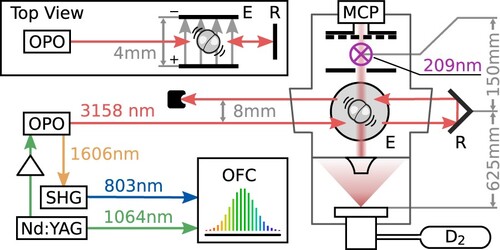
The upper left panel of Figure 2 shows a typical plot of the ion signal as a function of infrared laser frequency and time after the ionising laser pulse; a time trace at a single laser frequency (indicated with a red line) is shown in the lower left panel. The laser frequency in each time trace is determined using Equation (1(1) ${\nu }_i=(n_{1064}-n_{2s}/2)f_r+100\mathrm{MHz}-f_{\mathrm{bn},2s}/2,$(1) ) based on the beatnote frequency $f_{\mathrm{bn},2s}$ defined by the tunable radio-frequency reference and the average repetition rate $f_r$ recorded over the course of the scan. To avoid systematic shifts due to drifts of the signal strength, the laser frequencies in each scan are sampled in a random order. For this particular measurement, potentials of ±20 kV were applied to the field plates, resulting in a field strength of $9.69\times {10}^6\mathrm{V}/\mathrm{m}$, and the time trace for each of the 61 laser frequencies was averaged over ∼840 laser pulses, spread over two separate scans. Because the bottom extraction plate of the mass spectrometer has a hole to allow the molecules from the beam to enter, these molecules are ionised at a slightly lower electrical potential and thus arrive later than the background molecules ionised off the molecular beam axis. The two peaks in the time trace both correspond to ions with a mass of 4 amu, but only the second peak includes molecules from the molecular beam.

Figure 2. Data for a typical experimental spectrum, measured at an electric field strength of $9.69\times {10}^6\mathrm{V}/\mathrm{m}$. The upper left panel shows the D${}_2^{+}$ ion signal as a function of infrared laser frequency and time delay after the ionisation pulse, while the lower left panel shows a cut through at a single laser frequency. The peak at 2.94 µs corresponds to $v^{\prime }=1,N^{\prime }=2$ D${}_2$ in the molecular beam. Integrating over this peak and subtracting the baseline at each laser frequency results in the spectrum shown in black in the upper right panel. The spectrum is fit using the model described in Section 3.6, resulting in the red curve. Residuals of this fit are shown in the lower right panel. For comparison, a spectrum measured at zero electric field is also shown in the upper right panel in gray, with the corresponding model fit in pink.

To extract the infrared spectrum from the time traces, we integrate over the second peak and subtract the background determined by integrating over two regions symmetric around the same peak. The resulting spectrum is shown in the upper right panel in black. The spectrum contains two resolved peaks: the higher frequency peak is due to excitation by the outgoing infrared beam, and the lower frequency peak results from the returning infrared beam after retroreflection. A fit to the experimental data using multiple equal-width Gaussian functions is shown in red, and the residuals of this fit are shown in the lower right panel. More details on the fit are provided in Section 3.6. The gray curve in the upper right panel shows a second experimental spectrum that was measured under similar conditions but with no potential difference between the field plates; a multi-Gaussian fit to this spectrum is shown in pink. Without the electric field, the observed ion signal integrated over the entire spectrum is a factor of eight lower, and to achieve the signal to noise level shown, each point in the spectrum was averaged over eight times more pulses. In addition to the intensity difference, a clear frequency shift is observed between the two spectra. Based on the analysis described in Section 3.6, this offset is found to be quantitatively consistent with the expected differential dc Stark shift between the ground and excited state levels.

3. Analysis of the spectra

3.1. Zero-field Hamiltonian

To analyse the measured spectra, we construct an effective Hamiltonian model that describes the unresolved hyperfine structure as well as the molecule's interaction with the static electric field and laser field. A Python-based implementation of this model can be found in the Supplemental Material.¹ At zero field, the hyperfine structure for each rovibrational state can be modelled by the Hamiltonian [10] (2) $\begin{array}{rl}{\hat{H}}_0& =\sum _{\alpha =1}^2{c}_{\alpha ,vN}\hat{N}\cdot {\hat{I}}_{\alpha }+\sum _{\alpha =1}^2\frac{e{Q}_{\alpha }{q}_{0,vN}\sqrt{6}}{4I_{\alpha }(2I_{\alpha }-1)}{T}_{q=0}^2({\hat{I}}_{\alpha },{\hat{I}}_{\alpha })\\ & -S_{vN}\sqrt{6}{T}_{q=0}^2({\hat{I}}_1,{\hat{I}}_2),\end{array}$(2) where $\hat{N}$ is the rotational angular momentum operator and ${\hat{I}}_1$ and ${\hat{I}}_2$ are the nuclear spin operators. For the D${}_2$ molecule, the nuclear spins are $I_1=I_2=1$. The Hamiltonian is evaluated within the basis set described with the quantum numbers $|N{I}_{T}F{M}_F⟩$, where $I_T$ describes the total nuclear spin operator ${\hat{I}}_T={\hat{I}}_1+{\hat{I}}_2$ and F and $M_F$ describe the total angular momentum operator $\hat{F}=\hat{N}+{\hat{I}}_T$. Matrix elements for the terms in Equation (2(2) $\begin{array}{rl}{\hat{H}}_0& =\sum _{\alpha =1}^2{c}_{\alpha ,vN}\hat{N}\cdot {\hat{I}}_{\alpha }+\sum _{\alpha =1}^2\frac{e{Q}_{\alpha }{q}_{0,vN}\sqrt{6}}{4I_{\alpha }(2I_{\alpha }-1)}{T}_{q=0}^2({\hat{I}}_{\alpha },{\hat{I}}_{\alpha })\\ & -S_{vN}\sqrt{6}{T}_{q=0}^2({\hat{I}}_1,{\hat{I}}_2),\end{array}$(2) ) can be computed using [20] (3) $\begin{array}{rl}& ⟨N{I}_{T}F{M}_F|\hat{N}\cdot {\hat{I}}_{\alpha }|N{I}_T^{\prime }F{M}_F⟩=-(-1{)}^{N+I_T+F+I_1+I_2+I_T^{\ast }}\\ & \times \sqrt{N(N+1)(2N+1)I_{\alpha }(I_{\alpha }+1)(2I_{\alpha }+1)}\\ & \times \sqrt{(2I_T+1)(2I_T^{\prime }+1)}\left\{\begin{array}{ccc}{I}_T& I_T^{\prime }& 1\\ I_{\alpha }& I_{\alpha }& I_{3-\alpha }\end{array}\right\}\\ & \times \left\{\begin{array}{ccc}N& N& 1\\ I_T^{\prime }& I_T& F\end{array}\right\}\end{array}$(3) (4) $\begin{array}{rl}& ⟨N{I}_{T}F{M}_F|\frac{\sqrt{6}}{4I_{\alpha }(2I_{\alpha }-1)}{T}_{q=0}^2({\hat{I}}_{\alpha },{\hat{I}}_{\alpha })|N^{\prime }{I}_T^{\prime }F{M}_F⟩\\ & =(-1{)}^{N^{\prime }+I_T+F+N+I_1+I_2+I_T^{\ast }}\\ & \times \sqrt{\frac{(2I_{\alpha }+3)(2I_{\alpha }+2)(2I_{\alpha }+1)}{2I_{\alpha }(2I_{\alpha }-1)}}\\ & \times \frac{1}{4}\sqrt{(2N+1)(2N^{\prime }+1)(2I_T+1)(2I_T^{\prime }+1)}\\ & \times \left(\begin{array}{ccc}N& 2& N^{\prime }\\ 0& 0& 0\end{array}\right)\left\{\begin{array}{ccc}{I}_T& I_T^{\prime }& 2\\ I_{\alpha }& I_{\alpha }& I_{3-\alpha }\end{array}\right\}\left\{\begin{array}{ccc}N& N^{\prime }& 2\\ I_T^{\prime }& I_T& F\end{array}\right\}\end{array}$(4) (5) $\begin{array}{rl}& ⟨N{I}_{T}F{M}_F|\sqrt{6}{T}_{q=0}^2({\hat{I}}_1,{\hat{I}}_2)|N^{\prime }{I}_T^{\prime }F{M}_F⟩\\ & =(-1{)}^{N^{\prime }+I_T+F+N}\\ & \times \sqrt{I_1(I_1+1)(2I_1+1)I_2(I_2+1)(2I_2+1)}\\ & \times \sqrt{30(2N+1)(2N^{\prime }+1)(2I_T+1)(2I_T^{\prime }+1)}\\ & \times \left(\begin{array}{ccc}N& 2& N^{\prime }\\ 0& 0& 0\end{array}\right)\left\{\begin{array}{ccc}{I}_T& I_T^{\prime }& 2\\ I_1& I_1& 1\\ I_2& I_2& 1\end{array}\right\}\left\{\begin{array}{ccc}N& N^{\prime }& 2\\ I_T^{\prime }& I_T& F\end{array}\right\},\end{array}$(5) where $I_T^{\ast }$ is $I_T^{\prime }$ for $\alpha =1$ and $I_T$ for $\alpha =2$. While the hyperfine operators can potentially couple levels in different rotational states, the effect on the eigenenergies and eigenstates is negligible, so for simplicity, rotational terms are omitted from the Hamiltonian. Hyperfine parameters $c_{D,vN}$ ($-c_{\mathrm{nsr}}$), $e{Q}_D{q}_{0,vN}$, and $S_{vN}$ ($c_{\mathrm{dip}}$) for $v^{\prime }=1,N^{\prime }=2$ are taken from Jóźwiak et al. [21]; no parameters are needed for $v^{″}=0,N^{″}=0$, since all matrix elements of ${\hat{H}}_0$ within $N^{″}=0$ are zero. Because the second and third terms of Equation (2(2) $\begin{array}{rl}{\hat{H}}_0& =\sum _{\alpha =1}^2{c}_{\alpha ,vN}\hat{N}\cdot {\hat{I}}_{\alpha }+\sum _{\alpha =1}^2\frac{e{Q}_{\alpha }{q}_{0,vN}\sqrt{6}}{4I_{\alpha }(2I_{\alpha }-1)}{T}_{q=0}^2({\hat{I}}_{\alpha },{\hat{I}}_{\alpha })\\ & -S_{vN}\sqrt{6}{T}_{q=0}^2({\hat{I}}_1,{\hat{I}}_2),\end{array}$(2) ) couple basis states with different $I_T$ quantum numbers, eigenstates are labelled with ${\tilde{I}}_T$ corresponding to $I_T$ of the basis state with the greatest contribution.

3.2. Interactions with external fields

The electric field in the spectroscopy region is a combination of the static field from the plates and the oscillating field of the laser. Both fields are parallel and are assumed to lie along the $\hat{Z}$ axis. The static field is treated as being uniform in the region of interest, and the laser field is approximated as a plane wave travelling in the $\hat{Y}$ direction, resulting in a total electric field given by (6) $\begin{array}{r}{E}_Z=E_{\mathrm{static}}+\sqrt{{\mu }_{0}cI/2}(e^{2\pi \nu i(Y/c-t)}+e^{-2\pi \nu i(Y/c-t)}),\end{array}$(6) where ${\mu }_{0}c\approx 377\mathrm{\Omega }$ is the vacuum impedance, I is the laser intensity and ν is the optical frequency.

Field interactions can be defined with the help of Wigner $\mathfrak{D}$ matrices for the Euler angles ω of the internal $\hat{x},\hat{y},\hat{z}$ molecular axes relative to the space-fixed $\hat{X},\hat{Y},\hat{Z}$ axes. These define the relationship between spherical tensor operators defined in space-fixed coordinates (denoted with a p subscript) and those defined in molecule-fixed coordinates (denoted with a q subscript) [22]. (7) $\begin{array}{rl}{T}_q^k& =\sum _p{\mathfrak{D}}_{pq}^k(\omega )T_p^k\end{array}$(7) (8) $\begin{array}{rl}{T}_p^k& =\sum _q{{\mathfrak{D}}_{pq}^k}^{\ast }(\omega )T_q^k\end{array}$(8) Matrix elements for ${{\mathfrak{D}}_{pq}^k}^{\ast }(\omega )=(-1{)}^{p-q}{\mathfrak{D}}_{-p,-q}^k(\omega )$ between levels of the $X{}^1{\mathrm{\Sigma }}^{+}$ state of D${}_2$ can be computed using [20] (9) $\begin{array}{rl}& ⟨N{I}_{T}F{M}_F|{{\mathfrak{D}}_{pq}^k}^{\ast }(\omega )|N^{\prime }{I}_T{F}^{\prime }{M}_F^{\prime }⟩=(-1{)}^{F-M_F+I_T+F^{\prime }+k}\\ & \times \sqrt{(2F+1)(2F^{\prime }+1)(2N+1)(2N^{\prime }+1)}\\ & \times \left(\begin{array}{ccc}F& k& F^{\prime }\\ -M_F& p& M_F^{\prime }\end{array}\right)\left\{\begin{array}{ccc}F& F^{\prime }& k\\ N^{\prime }& N& I_T\end{array}\right\}\left(\begin{array}{ccc}N& k& N^{\prime }\\ 0& q& 0\end{array}\right)\end{array}$(9) Note that the last 3-j symbol (and thus the matrix element) is only non-zero if q = 0.

3.3. Polarisability matrix elements

The interaction of the molecule's polarisability tensor with an external electric field is given by (10) $\begin{array}{rl}{\hat{H}}_{\mathrm{pol}}& =-\frac{1}{2}(\alpha -\gamma /3)({E_x}^2+{E_y}^2)-\frac{1}{2}(\alpha +2\gamma /3){E_z}^2\\ & =-\frac{\alpha }{2}({E_x}^2+{E_y}^2+{E_z}^2)-\frac{\gamma }{6}(2{E_z}^2-{E_x}^2-{E_y}^2)\\ & =-(\frac{\alpha }{2}{{\mathfrak{D}}_{00}^0}^{\ast }(\omega )+\frac{\gamma }{3}{{\mathfrak{D}}_{00}^2}^{\ast }(\omega )){E_Z}^2.\end{array}$(10) Diagonal and off-diagonal components of the mean polarisability α and the polarisability anisotropy γ computed by Raj et al. are used in the analysis [23]. The ground-state D${}_2$ polarisability reported in this work agrees with the earlier prediction by Kołos and Wolniewicz to within 0.1% [24]. The polarisability Hamiltonian results in both Stark shifts to the individual states as well as transition moments. The Stark shift is dominated by the static field $E_{\mathrm{static}}$, which is 2–3 orders of magnitude larger than the laser field and thus produces a shift that is at least ${10}^4$ times larger than the shift due to the laser field alone. The ${E_Z}^2$ cross term $2E_{\mathrm{static}}\sqrt{{\mu }_{0}cI/2}(e^{2\pi \nu i(Y/c-t)}+e^{-2\pi \nu i(Y/c-t)})$ drives the transition moments relevant to this experiment.

3.4. Quadrupole transition moments

The interaction between the molecule's quadrupole moment and an external electric field gradient is given by (11) $\begin{array}{rl}{\hat{H}}_{\mathrm{quad}}& =-\frac{1}{2}\sum _{\alpha ,i,j}{q}_{\alpha }{R}_{i,\alpha }{R}_{j,\alpha }{\mathrm{\partial }}_i{E}_j\\ & =-\frac{1}{2}\sum _{\alpha }{q}_{\alpha }{T}^2(R_{\alpha },R_{\alpha })\cdot T^2(\mathrm{\nabla }E)\end{array}$(11) where $q_{\alpha }$ and $R_{\alpha }$ represent the charge and position, respectively, of each particle in the molecule, and [22] (12) $\begin{array}{rl}& T^2(R_{\alpha },R_{\alpha })\cdot T^2(\mathrm{\nabla }E)\\ & =\sum _p(-1{)}^p{T}_{-p}^2(R_{\alpha },R_{\alpha })T_p^2(\mathrm{\nabla }E)\\ & =\sum _{pq}(-1{)}^p{{\mathfrak{D}}_{-p,q}^2}^{\ast }(\omega )T_q^2(R_{\alpha },R_{\alpha })T_p^2(\mathrm{\nabla }E).\end{array}$(12) Only the q = 0 component of $T_q^2(R_{\alpha },R_{\alpha })$ results in non-zero matrix elements within the $X{}^1{\mathrm{\Sigma }}^{+}$ state (see Equation (9(9) $\begin{array}{rl}& ⟨N{I}_{T}F{M}_F|{{\mathfrak{D}}_{pq}^k}^{\ast }(\omega )|N^{\prime }{I}_T{F}^{\prime }{M}_F^{\prime }⟩=(-1{)}^{F-M_F+I_T+F^{\prime }+k}\\ & \times \sqrt{(2F+1)(2F^{\prime }+1)(2N+1)(2N^{\prime }+1)}\\ & \times \left(\begin{array}{ccc}F& k& F^{\prime }\\ -M_F& p& M_F^{\prime }\end{array}\right)\left\{\begin{array}{ccc}F& F^{\prime }& k\\ N^{\prime }& N& I_T\end{array}\right\}\left(\begin{array}{ccc}N& k& N^{\prime }\\ 0& q& 0\end{array}\right)\end{array}$(9) )) This component is related to the quadrupole moment operator eQ commonly quoted in literature (see, for example, Equation (24) in Jóźwiak et al. [21]) by the equation (13) $\begin{array}{rl}eQ& =\sum _{\alpha }{q}_{\alpha }({z_{\alpha }}^2-({x_{\alpha }}^2+{y_{\alpha }}^2)/2)\\ & =\sqrt{\frac{3}{2}}\sum _{\alpha }{q}_{\alpha }{T}_{q=0}^2(R_{\alpha },R_{\alpha })\end{array}$(13) where $(x_{\alpha },y_{\alpha },z_{\alpha })$ represent the positions of the particles in molecule-fixed coordinates. The only non-zero Cartesian component of $\mathrm{\nabla }E$ for the field defined in Equation (6(6) $\begin{array}{r}{E}_Z=E_{\mathrm{static}}+\sqrt{{\mu }_{0}cI/2}(e^{2\pi \nu i(Y/c-t)}+e^{-2\pi \nu i(Y/c-t)}),\end{array}$(6) ) is ${\mathrm{\partial }}_Y{E}_Z$, which results in space-fixed $p=\pm 1$ components for the spherical tensor operator given by [22] (14) $\begin{array}{r}{T}_{p=\pm 1}^2(\mathrm{\nabla }E)=\frac{\pi \nu }{c}\sqrt{\frac{{\mu }_{0}cI}{2}}(e^{2\pi \nu i(Y/c-t)}-e^{-2\pi \nu i(Y/c-t)}).\end{array}$(14) All other components ($p\ne \pm 1$) are zero. Combining the previous four equations results in the quadrupole interaction Hamiltonian (15) $\begin{array}{rl}{\hat{H}}_{\mathrm{quad}}& =-\frac{\pi \nu eQ}{c\sqrt{6}}\sqrt{\frac{{\mu }_{0}cI}{2}}(e^{2\pi \nu i(Y/c-t)}-e^{-2\pi \nu i(Y/c-t)})\\ & \times ({{\mathfrak{D}}_{10}^2}^{\ast }(\omega )+{{\mathfrak{D}}_{-10}^2}^{\ast }(\omega )).\end{array}$(15) The off-diagonal quadrupole moment $⟨v^{\prime }=1,N^{\prime }=2|eQ|v^{″}=0,N^{″}=0⟩=0.0682023\mathrm{e}{{\mathrm{a}}_0}^2$ computed by Jóźwiak et al. [21] is used to model the quadrupole component of the transition.

3.5. Integrated absorption cross sections

The interaction Hamiltonians can be converted to integrated cross sections (with dimensions of area × frequency/molecule) to enable comparisons to each other and to values from the existing literature. Assuming constant-intensity on-resonance illumination for a duration τ, the excitation probability in the weak field limit is given by (16) $P=\frac{{\tau }^2}{{\hslash }^2}|⟨\varphi |e^{i\hat{H}t/\hslash }{\hat{H}}^{\prime }{e}^{-i\hat{H}t/\hslash }|{\varphi }^{\prime }⟩{|}^2$(16) where ${\hat{H}}^{\prime }$ is the interaction Hamiltonian, $\hat{H}$ is the Hamiltonian excluding the interaction, ϕ is the excited state, and ${\varphi }^{\prime }$ is the ground state. The unitary transformation $e^{-i\hat{H}t/\hslash }$ eliminates the time variation of one of the terms in the factor $(e^{2\pi \nu i(Y/c-t)}\pm e^{-2\pi \nu i(Y/c-t)})$ appearing in Equations (6(6) $\begin{array}{r}{E}_Z=E_{\mathrm{static}}+\sqrt{{\mu }_{0}cI/2}(e^{2\pi \nu i(Y/c-t)}+e^{-2\pi \nu i(Y/c-t)}),\end{array}$(6) ) and (15(15) $\begin{array}{rl}{\hat{H}}_{\mathrm{quad}}& =-\frac{\pi \nu eQ}{c\sqrt{6}}\sqrt{\frac{{\mu }_{0}cI}{2}}(e^{2\pi \nu i(Y/c-t)}-e^{-2\pi \nu i(Y/c-t)})\\ & \times ({{\mathfrak{D}}_{10}^2}^{\ast }(\omega )+{{\mathfrak{D}}_{-10}^2}^{\ast }(\omega )).\end{array}$(15) ) and doubles the frequency of the other; by invoking the rotating wave approximation, this entire factor can therefore be treated as being equal to one when evaluating Equation (16(16) $P=\frac{{\tau }^2}{{\hslash }^2}|⟨\varphi |e^{i\hat{H}t/\hslash }{\hat{H}}^{\prime }{e}^{-i\hat{H}t/\hslash }|{\varphi }^{\prime }⟩{|}^2$(16) ). Over the time τ, a molecule is illuminated with ${\tau }^{2}I/(h\nu )$ photons per unit area and per unit frequency, and on average, P photons are absorbed per molecule in the ${\varphi }^{\prime }$ initial quantum state. The cross section of a molecule in this specific initial state is thus given by (17) $\sigma =\frac{P}{{\tau }^{2}I/(h\nu )}=\frac{4{\pi }^2\nu }{hI}|⟨\varphi |e^{i\hat{H}t/\hslash }{\hat{H}}^{\prime }{e}^{-i\hat{H}t/\hslash }|{\varphi }^{\prime }⟩{|}^2$(17) which is independent of the illumination time τ. To compute the average cross section for a molecule in the sample, σ should be multiplied by the fraction of the molecules in the given initial state.

As a specific example, we consider a $N=2\leftarrow N^{\prime }=0$ transition driven by the quadrupole interaction with hyperfine couplings excluded (i.e. $I_1=I_2=0$). All molecules are assumed to initially be in the $N^{\prime }=0,M_N^{\prime }=0$ ground state. The sum of the squared matrix elements of the interaction Hamiltonian over all excited-state $M_N$ levels is given by (18) $\begin{array}{rl}& \sum _{M_N}|⟨2,M_N|e^{i\hat{H}t/\hslash }{\hat{H}}_{\mathrm{quad}}{e}^{-i\hat{H}t/\hslash }|0,0⟩{|}^2\\ & =\frac{{\pi }^2{\nu }^2{e}^2{Q}^2{\mu }_{0}I}{30c},\end{array}$(18) which results in an integrated cross section (19) $\sigma (N=2,N^{\prime }=0)=\frac{2{\mu }_0{\pi }^4{\nu }^3{e}^2{Q}^2}{15hc},$(19) in agreement with Equation (17) of Jóźwiak et al. [21].

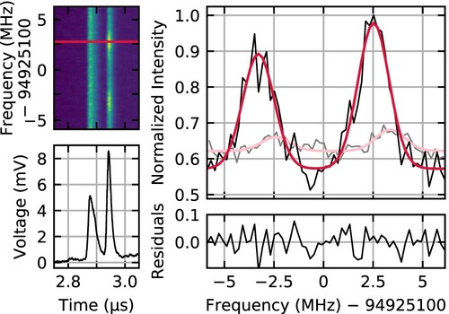
3.6. Vibrational transitions in an electric field

Using the Hamiltonian operators defined above, we can model the $M_F$-state resolved transition frequencies and intensities in a static electric field for both quadrupole and induced dipole transitions. The left panel of Figure 3 shows the transition frequencies relative to the line center for the components of the S${}_1$(0) ($v^{\prime }=1,N^{\prime }=2\leftarrow v^{″}=0,N^{″}=0$) transition as a function of electric field strength. For the $v^{″}=0,N^{″}=0$ ground state, all levels are degenerate, and their energies shift in an electric field by $-{\alpha }^{″}{E}^2/2$, where ${\alpha }^{″}=5.34934361{\mathrm{e}}^2{{\mathrm{a}}_0}^2/{\mathrm{E}}_{\mathrm{h}}$ is the mean polarisability of the rovibrational state [23]. At zero field, the $|{\tilde{I}}_T^{\prime },F^{\prime }⟩$ levels of the $N^{\prime }=2$ excited state are (in order of increasing energy) $|0,2⟩$, $|2,4⟩$, $|2,0⟩$, $|2,1⟩$, $|2,3⟩$, and $|2,2⟩$, with energies independent of the $M_F^{\prime }$ quantum number. When a field is applied, these levels shift according to their $M_F^{\prime }$ quantum numbers and, at higher fields, transition into a Paschen-Back regime where $M_N^{\prime }$ becomes a good quantum number. The right panel shows spectra due to electric quadrupole (red) and induced electric dipole (blue) transitions computed at field strengths of 0 V/m, $3.36\times {10}^6\mathrm{V}/\mathrm{m}$ (the lowest non-zero field used in the experiment), and $9.69\times {10}^6\mathrm{V}/\mathrm{m}$ (the maximum field used in the experiment). These field strengths are indicated in the left panel by vertical gray bars, and the spectra are shown in the same order in the right panel. Each of the six $v^{″}=0,N^{″}=0$ ground-state levels are assumed to contain 1/6 of the total population, and the spectra are computed assuming a Gaussian line shape with a width of $\sigma =3\mathrm{kHz}$. While no induced dipole transitions are possible at zero field, at the maximum field strength, the integrated strength of the induced dipole transitions is about 8.4 times larger than for the quadrupole transitions. Because the two types of transitions obey different selection rules, different peaks are allowed or more prominent for each type. At the highest field strength, in particular, quadrupole transitions are primarily to the $|M_N^{\prime }|=1$ levels and induced dipole transitions are primarily to the $M_N^{\prime }=0$ levels due to the respective $\mathrm{\Delta }{M}_N=\pm 1$ and $\mathrm{\Delta }{M}_N=0$ selection rules.

Figure 3. S${}_1$(0) quadrupole and induced-dipole transitions in an electric field. The left panel shows the $M_F^{\prime }$-resolved energies of the $v^{\prime }=1,N^{\prime }=2$ excited state levels relative to the $v^{″}=0,N^{″}=0$ ground state levels, which all shift equally in an electric field. At higher fields, $M_N^{\prime }$ becomes an approximately good quantum number, leading to the levels grouping into three sets, corresponding to $M_N^{\prime }=0$, $|M_N^{\prime }|=1$, and $|M_N^{\prime }|=2$. The right panel shows simulated spectra due to electric quadrupole (red) and induced-dipole (blue) transition moments computed at field strengths of (from left to right) 0 V/m, $3.36\times {10}^6\mathrm{V}/\mathrm{m}$, and $9.69\times {10}^6\mathrm{V}/\mathrm{m}$. The same field strengths are indicated in the left panel with vertical gray bars.

Each measured spectrum is fit using a sum of multiple Gaussian functions with relative intensities and frequency offsets determined using the model above. To account for both the outgoing and returning infrared beams, which have different optical frequencies in the molecule frame due to the Doppler shift, each Gaussian is included twice, with a global frequency offset and two global intensity scaling factors that are determined in the fit. The fitting function can be described by (20) $\begin{array}{rl}S(\nu )=\sum _i{I}_i(& A_o{e}^{-(\nu -{\nu }_0-{\nu }_i-\mathrm{\Delta }/2{)}^2/(2{\sigma }^2)}\\ +& A_r{e}^{-(\nu -{\nu }_0-{\nu }_i+\mathrm{\Delta }/2{)}^2/(2{\sigma }^2)})+S_0\end{array}$(20) where $S(\nu )$ is the spectral intensity at optical frequency ν and the six fitting parameters are ${\nu }_0$ (the transition frequency), Δ (frequency offset between the two Doppler-shifted peaks), σ (the Gaussian linewidth), $A_o$ and $A_r$ (amplitudes of the peaks due to the outgoing and returning infrared beams, respectively), and $S_0$ (a baseline offset). Pairs of $(I_i,{\nu }_i)$ represent the intensity and frequency offset, respectively, of each $M_F$-state resolved transition. This approach automatically accounts for both the residual Doppler shift as well as the dc Stark shift: the ${\nu }_0$ determined in the fit nominally describes the zero-field excitation frequency for molecules at zero transverse velocity. 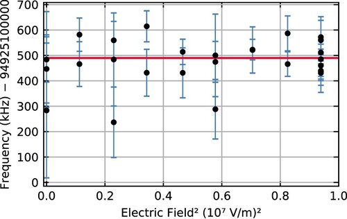Figure 4 shows the ${\nu }_0$ determined in fits of 28 separate spectra at nine different field strengths as a function of the square of the electric field strength; error bars indicate 1-σ statistical errors for each point. The weighted average of all ${\nu }_0$ is 94,925,100,490(12) kHz, which is indicated by the red horizontal line.

Figure 4. Absolute zero-field transition frequencies extracted from 28 individual spectra recorded at nine different field strengths. Each spectrum is fit with a model that accounts for the Stark shift at the field strength used in that particular measurement. The weighted average of the individual measurements is indicated by the red horizontal line.

4. Systematic shifts

A number of additional systematic shifts and uncertainties have been considered in the analysis. Several potential shifts are found to have a negligible contribution to the absolute frequency or overall uncertainty. The ac Stark shift is expected to be less than 1 Hz at an estimated peak infrared beam intensity of 0.2 W/mm${}^2$. At an estimated molecular beam density of $4\times {10}^{17}{\mathrm{m}}^{-3}$, the density shift is estimated to be approximately $-1$ Hz based on the $-2.5\times {10}^{-3}{\mathrm{cm}}^{-1}/\mathrm{amagat}$ slope reported by Maddaloni et al. [25]. The Larmor frequency of a deuteron in the $\sim 3$µT residual magnetic field is only 20 Hz, so any Zeeman shifts must be less than 40 Hz. Uncertainties in the relative strengths of the quadrupole and polarisability transition moments, estimated to be less than 0.1% for each transition moment, contribute less than 30 Hz of additional uncertainty to the transition frequency determined from the experimental data. Errors in the absolute frequency of the radio-frequency reference are expected to contribute less than 500 Hz to the overall uncertainty.

The largest systematic contribution to the overall uncertainty is due to the uncertainty of the spacing between the field plates, which affects the static electric field strength and thus the Stark shift. Using the digital position read out on the table of a milling machine, together with a dial test indicator, the plate spacing was determined to be $4.13\pm 0.03\mathrm{mm}$. If plate spacings of 4.16 mm and 4.10 mm are assumed in the analysis, which decreases or increases the field strength assumed for each measurement, the average of the transition frequencies determined in the spectral fits decreases or increases by 10 kHz, respectively. While the applied potentials, the fringe field at the plates, and the polarisability of the molecules can also affect the overall Stark shift and thus the frequencies determined in the fits, the uncertainties for these contributions are much smaller: while the fractional uncertainty of the plate spacing is 0.7%, the fractional uncertainties of the other components is less than 0.1%.

Ambiguities in the relative detection efficiency for the unresolved hyperfine components of the transition also contribute to the overall uncertainty. The relative intensities used for the spectral fits are based on the implicit assumption that all molecules excited to $v^{\prime }=1$ are detected with equal efficiency. If all $M_F^{\prime }$ components within each ${\tilde{I}}_T^{\prime },F^{\prime }$ level are equally populated during the ionisation step, this assumption will be true, but if the uneven $M_F^{\prime }$ distribution following the infrared excitation persists until ionisation, molecules in some $v^{\prime }=1$ levels could be detected more efficiently than those in others. We estimate the shift of the measured line frequency due to this effect by calculating the transition center of mass with each vibrational transition frequency weighted by the product of the vibrational transition strength and the two-photon electronic transition strength. For each unique transition frequency, the vibrational transition strength includes all transitions from any ground state $F^{″},M_F^{″}$ level to a coherent superposition of all degenerate $v^{\prime }=1$ levels contributing to the line, and the two-photon transition strength includes transitions from the coherent superposition to any $I_T,F,M_F$ level in the EF, v = 0, N = 2 state. At zero electric field, the coherent superposition covers all $M_F^{\prime }$ levels in each ${\tilde{I}}_T^{\prime },F^{\prime }$ level, but in a field, only pairs of levels with equal and opposite $M_F^{\prime }$ quantum numbers remain degenerate. With no potential between the field plates, the $v^{\prime }=1$ coherent superposition can remain the same between the infrared excitation and ionisation, but if there is a field in the infrared excitation region, the molecules must leave this field to reach the ionisation region. For these calculations, we assume that the coherent superposition excited in the field transitions adiabatically to the corresponding zero-field state. Based on these assumptions, the transition center of mass at zero field is expected to shift by +5.2 kHz relative to the case where all $v^{\prime }=1$ molecules are detected with equal probability, a center-of-mass shift of −1.5 kHz is expected for the smallest non-zero electric field used in the experiments ($3.36\times {10}^6\mathrm{V}/\mathrm{m}$), and a shift of −4.5 kHz is expected for the largest electric field ($9.69\times {10}^6\mathrm{V}/\mathrm{m}$). To account for these potential shifts, we include an additional 6 kHz uncertainty in the error budget.

A residual Doppler shift due to manufacturing tolerances of the corner cube retroreflector has also been included in the error budget. The retroreflector (Newport UBBR2.5-1S) has a specified parallelism of $1^{″}$. At a molecular beam velocity of 2100 m/s, this angular deviation results in a potential residual Doppler shift of ±1.6 kHz.

The optical frequency determined in the fit in Section 3.6 corresponds to the laser frequency required to excite the S${}_1$(0) transition in a molecule with zero velocity along the laser axis at zero electric field. This frequency is corrected downward by $h{\nu }_0^2/(2m{c}^2)=5\mathrm{kHz}$ to account for the photon energy lost to imparting kinetic energy to the molecule (recoil shift) and upward by ${\nu }_0(v/c{)}^2/2=2.3\mathrm{kHz}$ to account for the second-order Doppler shift, resulting in an absolute rest-frame transition frequency of 94,925,100,487 kHz. A Pythagorean sum of the statistical uncertainty (12 kHz), the uncertainty due to the field strength (10 kHz), hyperfine effects (6 kHz), and retroreflection quality (2 kHz) results in an overall uncertainty of 17 kHz. All contributions to the absolute transition frequency and its uncertainty are summarised in Table 1.

Table 1. Frequency and uncertainty contributions to the measured S${}_1$(0) transition frequency.

Contribution	Frequency (kHz)	σ (kHz)
Doppler-corrected peak position	94,925,100,490	12
Electric field strength	0	10
Hyperfine	0	6
First-order Doppler	0	2
Frequency reference error	0	<0.5
ac Stark, Zeeman, Pressure,	0	<0.1
Transition strength
Recoil	−5.0	0
Second-order Doppler	+2.3	<0.5
Total	94,925,100,487	17

5. Comparison to previous works

Table 2 shows a comparison of the D${}_2$ S${}_1$(0) transition frequency determined in this work and those measured or computed previously. The most recent direct measurement of the S${}_1$(0) transition frequency by Maddaloni et al. [25] deviates from our measurement by seven times the reported uncertainty. A second, independent experimental estimate of the transition frequency can be found by combining the Q${}_1$(2) transition frequency reported Niu et al. [26] with the difference of the S${}_2$(0) and Q${}_2$(2) transition frequencies reported by Mondelain et al. [12]. The resulting frequency has a slightly smaller overall uncertainty and agrees with the frequency determined in this work to within experimental uncertainty. Komasa et al. [1] have determined the transition frequency using ab-initio methods, and their value also agrees with the value reported here to within the given uncertainty.

Table 2. Comparison between the D${}_2$ S${}_1$(0) transition frequency determined in the present work and previous experimental and theoretical values.

	Frequency (MHz)	Deviation (MHz)
This work	94,925,100.487(17)
Ref. [25] (Exp.)	94,925,144.7(6.0)	−44.2(6.0)
Refs. [12,26] (Exp.)	94,925,103.5(4.5)	−3.0(4.5)
Ref. [1] (Theo.)	94,925,100.0(4)	0.5(4)

6. Conclusion and outlook

We report a high-precision direct measurement of a fundamental band vibrational transition frequency of a homonuclear isotope of molecular hydrogen. The current study focussed on the S${}_1$(0) transition, but a more interesting target (which was not investigated in the present work due to a mundane technical limitation) is the Q${}_1$(0) transition at 89.74638 THz. Because the Q${}_1$(0) transition is forbidden by quadrupole selection rules, previous high-precision spectroscopic measurements investigating quadrupole transitions have not been able to access this line. Compared to the S${}_1$(0) transition, Q${}_1$(0) has an induced dipole transition that is approximately 19 times stronger and has less than half the differential Stark shift. Additionally, the Q${}_1$(0) transition has no hyperfine structure. These three advantages would greatly reduce the three largest contributions to the frequency uncertainty of the present work, making it possible to determine the transition frequency with an uncertainty of less than 5 kHz under similar experimental conditions to those used here. The approach demonstrated here can also be applied to the same transitions in H${}_2$, where all transitions between para levels are free of hyperfine structure.

Acknowledgments

We gratefully acknowledge S. Kaufmann, K. Papendorf, and T. Zhong for lending us the UV ionisation laser and providing assistance with its operation. We also thank W. Ubachs for providing additional information on field-induced spectroscopy of molecular hydrogen.

Data availability statement

The data that support the findings of this study are available from the Edmond Open Research Data Repository at https://dx.doi.org/10.17617/3.7u.

Disclosure statement

No potential conflict of interest was reported by the author(s).

Correction Statement

This article has been corrected with minor changes. These changes do not impact the academic content of the article.

Notes

1 See Supplemental Material for a Python-based implementation of the effective Hamiltonian model described in Section 3

References

- J. Komasa, M. Puchalski, P. Czachorowski, G. Łach and K. Pachucki, Phys. Rev. A 100, 032519 (2019). doi:10.1103/PhysRevA.100.032519.
- W. Ubachs, J.C.J. Koelemeij, K.S.E. Eikema and E.J. Salumbides, J. Mol. Spectrosc. 320, 1–12 (2016). doi:10.1016/j.jms.2015.12.003.
- C.F. Cheng, Y.R. Sun, H. Pan, J. Wang, A.W. Liu, A. Campargue and S.M. Hu, Phys. Rev. A 85, 024501 (2012). doi:10.1103/PhysRevA.85.024501.
- D. Mondelain, S. Kassi, T. Sala, D. Romanini, D. Gatti and A. Campargue, J. Mol. Spectrosc. 326, 5–8 (2016). doi:10.1016/j.jms.2016.02.008.
- P. Wcisło, F. Thibault, M. Zaborowski, S. Wójtewicz, A. Cygan, G. Kowzan, P. Masłowski, J. Komasa, M. Puchalski, K. Pachucki, R. Ciuryło and D. Lisak, J. Quant. Spectrosc. Radiat. Transf.213, 41–51 (2018). doi:10.1016/j.jqsrt.2018.04.011.
- F.M.J. Cozijn, P. Dupré, E.J. Salumbides, K.S.E. Eikema and W. Ubachs, Phys. Rev. Lett. 120, 153002 (2018). doi:10.1103/PhysRevLett.120.153002.
- M.L. Diouf, F.M.J. Cozijn, B. Darquié, E.J. Salumbides and W. Ubachs, Opt. Lett. 44, 4733–4736 (2019). doi:10.1364/OL.44.004733.
- M. Zaborowski, M. Słowiński, K. Stankiewicz, F. Thibault, A. Cygan, H. Jóźwiak, G. Kowzan, P. Masłowski, A. Nishiyama, N. Stolarczyk, S. Wójtewicz, R. Ciuryło, D. Lisak and P. Wcisło, Opt. Lett. 45, 1603–1606 (2020). doi:10.1364/OL.389268.
- M.L. Diouf, F.M.J. Cozijn, K.F. Lai, E.J. Salumbides and W. Ubachs, Phys. Rev. Res. 2, 023209 (2020). doi:10.1103/PhysRevResearch.2.023209.
- A. Fast and S.A. Meek, Phys. Rev. Lett. 125, 023001 (2020). doi:10.1103/PhysRevLett.125.023001.
- T.P. Hua, Y.R. Sun and S.M. Hu, Opt. Lett. 45, 4863–4866 (2020). doi:10.1364/OL.401879.
- D. Mondelain, S. Kassi and A. Campargue, J. Quant. Spectrosc. Radiat. Transf. 253, 107020 (2020). doi:10.1016/j.jqsrt.2020.107020.
- A. Castrillo, E. Fasci and L. Gianfrani, Phys. Rev. A 103, 022828 (2021). doi:10.1103/PhysRevA.103.022828.
- M.F. Crawford and I.R. Dagg, Phys. Rev. 91, 1569–1570 (1953). doi:10.1103/PhysRev.91.1569.2.
- M.F. Crawford and R.E. MacDonald, Can. J. Phys. 36, 1022–1039 (1958). doi:10.1139/p58-111.
- R.W. Terhune and C.W. Peters, J. Mol. Spectrosc. 3, 138–147 (1959). doi:10.1016/0022-2852(59)90016-5.
- J.V. Foltz, D.H. Rank and T.A. Wiggins, J. Mol. Spectrosc. 21, 203–216 (1966). doi:10.1016/0022-2852(66)90138-X.
- P.J. Brannon, C.H. Church and C.W. Peters, J. Mol. Spectrosc. 27, 44–54 (1968). doi:10.1016/0022-2852(68)90018-0.
- H.L. Buijs and H.P. Gush, Can. J. Phys. 49, 2366–2375 (1971). doi:10.1139/p71-284.
- S.A. Meek, Ph. D. thesis, Freie Universität Berlin, 2010.
- H. Jóźwiak, H. Cybulski and P. Wcisło, J. Quant. Spectrosc. Radiat. Transf. 253, 107186 (2020). doi:10.1016/j.jqsrt.2020.107186.
- J. Brown and A. Carrington, in Rotational Spectroscopy of Diatomic Molecules (Cambridge University Press, Cambridge, UK, 2003), Chap. 5.
- A. Raj, H. Hamaguchi and H.A. Witek, J. Chem. Phys 148, 104308 (2018). doi:10.1063/1.5011433.
- W. Kołos and L. Wolniewicz, J. Chem. Phys. 46, 1426–1432 (1967). doi:10.1063/1.1840870.
- P. Maddaloni, P. Malara, E. De Tommasi, M. De Rosa, I. Ricciardi, G. Gagliardi, F. Tamassia, G. Di Lonardo and P. De Natale, J. Chem. Phys 133, 154317 (2010). doi:10.1063/1.3493393.
- M.L. Niu, E.J. Salumbides, G.D. Dickenson, K.S.E. Eikema and W. Ubachs, J. Mol. Spectrosc. 300, 44–54 (2014). doi:10.1016/j.jms.2014.03.011.