Consequences of approximating electron correlation effects

ABSTRACT

The effect of approximating electron correlation in few-electron systems is investigated using three wavefunctions: the many body wavefunction referred to as fully-correlated (FC), the Hartree Fock wavefunction (HF), and the Colle and Salvetti Jastrow-style wavefunction (CS) used in the derivation of the popular Lee, Yang and Parr (LYP) correlation functional. The electron correlation energy, static and dynamic Coulomb holes, various expectation values, and radial energy distributions (energy densities) are considered. It is shown that whilst the CS wavefunction can capture the behaviour of the wavefunction at the singularities of the Coulomb potential corresponding to the coalescence of two particles and decreases the area of the primary static Coulomb hole by nearly 30% compared to HF for He and Li${}^{+}$, it is unable to accurately model expectation values that depend on the whole of space and key features of the electron density behaviour in dynamic Coulomb holes and the energy density behaviour in energy distributions. These issues are amplified when considering the hydride ion and a system with the critical nuclear charge for binding.

GRAPHICAL ABSTRACT

KEYWORDS:

• Electron correlation
• two-electron systems
• Coulomb holes
• correlation energies

1. Introduction

Electron correlation energy represents a small fraction of the total energy of a quantum mechanical system, yet its inclusion is essential for achieving chemical accuracy in detailed studies of atoms and molecules. The lack of a usable analytical solution to the quantum mechanical many-body problem has led to an abundance of innovative and creative ideas to include electron correlation effects in many-body calculations. Löwdin defined electron correlation energy, $E_{\mathrm{corr}}$, as the difference between the exact, non-relativistic ground state energy, $E_{\mathrm{exact}}$, and the Hartree Fock (HF) energy, $E_{\mathrm{HF}}$ [1,2]: (1) $E_{\mathrm{corr}}=E_{\mathrm{exact}}-E_{\mathrm{HF}}.$(1) One of the most prominent theories to address the electron correlation challenge is approximate density functional theory (DFT) and one of the most popular correlation functionals is the LYP functional [3]. This functional is based on a formula derived by Colle and Salvetti (CS) to approximate the electron correlation energy for atoms and molecules [4]. There have been numerous detailed critiques of this formula, see for example [5–8], and recently, we reported an inability to improve or recalibrate either the Colle and Salvetti or LYP methods for anions [9]. The CS method is derived from approximating the exact wavefunction as the product of a Hartree Fock wavefunction and a Jastrow factor which aims to capture the electron correlation behaviour absent from HF theory. In fact, the majority of conventional quantum chemistry methods use the HF wavefunction as a reference, for example Møller-Plesset perturbation theory, coupled cluster theory, and configuration interaction methods, and a Jastrow-style factor has been used in a number of contexts. For a review on explicitly correlated electrons in molecules see [10].

Particularly challenging is capturing the long-range low density behaviour of anions, and it is known that the restricted HF hydride ion does not support a bound state [11] even though it was proven back in the 1970s that the energy of the hydride ion lies below the lowest continuum threshold [12]. The critical nuclear charge $Z_C$ for which an atomic system has at least one bound state has been studied extensively for two-electron systems (see for example, [13–15]) using high precision calculations that include the electron-electron distance in the coordinates (e.g. through the use of Hylleraas coordinates or perimetric coordinates); this type of calculation we refer to as fully-correlated (FC). Within the fixed nucleus approximation, $Z_C^{\mathrm{FC}}=0.91102822407725573(4)$ [14]. However, it wasn't until recently that the analogous critical nuclear charge for binding at the HF level of theory was accurately determined. The critical nuclear charge, corresponding to the energy at which the three-body system equals the lowest continuum threshold, is $Z_C^{\mathrm{HF}}$= 1.031 177 528 [16]. Given that the hydride ion is unbound at this level of theory [11, and references therein], the critical charge for binding at this level of theory must be greater than one. An alternative definition of the HF critical nuclear charge, is the point at which the occupied orbital energy becomes zero, which we will refer to as $Z_C^{{\mathrm{HF}}_0}$, and it was shown that this corresponds to a value of $Z_C^{{\mathrm{HF}}_0}$ = 0.828 161 008 [17]. Recently, the critical nuclear charge at the radial limit, a well-defined intermediate between HF and the FC solution of the non-relativistic Schrödinger equation, has been considered and shown to have a value of $Z_C^{\mathrm{radial}}=0.9487$ [18]. The radial limit corresponds to the best solution provided by a wave function that depends only on the single-particle radial coordinates $r_1$ and $r_2$, it accounts for the radial correlation but omits the angular correlation provided in the FC solution.

Coulomb holes have long remained an important descriptor in studying electron correlation [5,19–21] owing to their ease of conceptualising the effect of electron correlation on the inter-electronic separation. More recent work has explored secondary Coulomb holes in two-electron systems [22,23] revealing new information about these density holes and how electron correlation can act to bring electrons closer together. Coulomb holes characterise the error in electron density when described using HF theory and a key component of the CS method is their relation of the volume of the correlation hole to Wigner's exclusion volume in order to capture this important physical property. The Coulomb hole defined by Coulson and co-workers [19,24] is stated in terms of the radial electron-electron distribution function which does not explicitly account for the change in electron probability density as a function of the nucleus-electron distance. Dynamic Coulomb holes [5,6,25], more commonly referred to as correlation holes [26], offer an alternative description allowing for the non-uniformity of the two-electron density to be captured. Here we calculate dynamic Coulomb holes for a cation, a neutral atom and an anion to provide insight into how the two-electron density measured from the nucleus behaves as a function of Z, including at the critical stability point, $Z_C^{\mathrm{FC}}$. These exact dynamic Coulomb holes are compared to approximate dynamic Coulomb holes calculated using a formula derived from the CS wavefunction.

Expectation values may be a standard means of relating quantum mechanical calculations to observables measured by experiment, but important information is often lost about individual contributions that form the overall average (c.f. $r_{max}$ in the radial distribution function versus $⟨r⟩$). Electron correlation energy is always negative, evidenced by considering Löwdin's definition, Equation (1(1) $E_{\mathrm{corr}}=E_{\mathrm{exact}}-E_{\mathrm{HF}}.$(1) ), as the exact energy is always lower than the Hartree Fock energy. However, when electron correlation is ‘switched on’ in the FC method, is the effect always to reduce the energy at every point in coordinate space within a physical system? We answer this question by calculating energies at discrete points in coordinate space for both the FC and the HF method allowing for the electron correlation energy to be calculated at each of these points.

Thus the goal of this investigation is to explore the physical limitations of approximating electron correlation effects.

2. Theory and method

2.1. Fully-Correlated (FC), Hartree-Fock (HF), and Colle-Salvetti (CS) methods

The singlet ground states of helium and helium-like systems, within the clamped nucleus approximation, are investigated. The details of the implementation used for the FC method is described in [27], for the HF method in [16], and for the CS method in [4,9]. Atomic units (a.u.) are used throughout, where $m_e=\hslash =(4\pi {ϵ}_0{)}^{-1}=e=1$, and the atomic unit of energy is the Hartree ($E_h$) and the atomic unit of length is the Bohr ($a_0$). 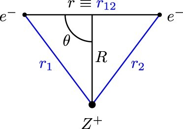Figure 1 shows the coordinates referred to throughout this investigation, the interparticle coordinates $\{r_1,r_2,r_{12}\}$ and the Jacobi coordinates, $r\equiv r_{12},R,\theta$.

Figure 1. Coordinates utilised in this work (i) Inter-particle coordinates, $r_1,r_2$ and $r_{12}$ and (ii) Jacobi coordinates $r\equiv r_{12},R$ and θ.

The HF wavefunction, ${\psi }_{\mathrm{HF}}$, is taken as the product (2) ${\mathrm{\Psi }}_{\mathrm{HF}}(r_1,r_2)=\psi (r_1)\psi (r_2),$(2) where the required anti-symmetry of the total wave function is embedded in the spin part which has been integrated out. The $\psi (r_i)$ have the form (3) $\psi (r_i)={\mathrm{e}}^{-\frac{1}{2}A{r}_i}\sum _{q=0}^{\mathrm{\infty }}C(q)L_q(A{r}_i),i=1\mathrm{or}2,$(3) and $r_1$ and $r_2$ are the nucleus-electron distances, $L_n(x)$ is a Laguerre polynomial of degree n and A is a non-linear variational parameter. The HF wavefunction (2(2) ${\mathrm{\Psi }}_{\mathrm{HF}}(r_1,r_2)=\psi (r_1)\psi (r_2),$(2) ) is substituted in the Roothaan-Hall equations in the case of RHF and the Pople-Nesbet equations for UHF. These are solved using an iterative self consistent field (SCF) procedure. The series solution method is used to calculate one-electron integrals and a derived analytical solution is used for the two-electron integrals [16]. All two-electron integrals were calculated using 200-digit ball arithmetic precision to enforce accuracy and allowing for rigorous error bounds for every integral. All RHF and UHF data presented in this work was calculated using 25-term wavefunctions with 64-digit precision throughout the SCF and parameter optimisation procedures.

The FC wavefunction, ${\mathrm{\Psi }}_{\mathrm{FC}}$ (which we take as $\approx {\mathrm{\Psi }}_{\mathrm{exact}}$), explicitly includes the electron-electron distance, $r_{12}$, and is written in terms of the perimetric coordinates, $z_i=r_j+r_k-r_i$, which are linear combinations of the inter-particle distances $r_1,r_2$ and $r_{12}$ by cyclic permutation; the perimetric coordinates are independent and each range from 0 to ∞. The FC wavefunction has the form: (4) $\begin{array}{rl}& {\mathrm{\Psi }}_{\mathrm{FC}}(z_1,z_2,z_3)\\ & ={\mathrm{e}}^{-\frac{1}{2}(\alpha z_1+\alpha z_2+2\alpha z_3)}\\ & \times \sum _{l,m,n=0}^{\mathrm{\infty }}A(l,m,n)\{L_l(\alpha z_1)L_m(\alpha z_2)\\ & +L_m(\alpha z_1)L_l(\alpha z_2)\}{L}_n(2\alpha z_3),\end{array}$(4) where α is a non-linear variational parameter introduced to increase the rate of convergence. The FC wavefunction (4(4) $\begin{array}{rl}& {\mathrm{\Psi }}_{\mathrm{FC}}(z_1,z_2,z_3)\\ & ={\mathrm{e}}^{-\frac{1}{2}(\alpha z_1+\alpha z_2+2\alpha z_3)}\\ & \times \sum _{l,m,n=0}^{\mathrm{\infty }}A(l,m,n)\{L_l(\alpha z_1)L_m(\alpha z_2)\\ & +L_m(\alpha z_1)L_l(\alpha z_2)\}{L}_n(2\alpha z_3),\end{array}$(4) ) is substituted into the Schrödinger equation and the resulting generalised eigenvalue equation for the fully-correlated system is solved using a series solution method described by Cox et al. [27] and based on the original work of Pekeris [28]. The standard Laguerre recursion relations are used to eliminate the powers and derivatives of the variables, resulting in a 33-term recursion relation between the coefficients $A(l,m,n)$ in (4(4) $\begin{array}{rl}& {\mathrm{\Psi }}_{\mathrm{FC}}(z_1,z_2,z_3)\\ & ={\mathrm{e}}^{-\frac{1}{2}(\alpha z_1+\alpha z_2+2\alpha z_3)}\\ & \times \sum _{l,m,n=0}^{\mathrm{\infty }}A(l,m,n)\{L_l(\alpha z_1)L_m(\alpha z_2)\\ & +L_m(\alpha z_1)L_l(\alpha z_2)\}{L}_n(2\alpha z_3),\end{array}$(4) ). All FC results presented in this work are calculated using a 4389-term wavefunction.

The CS wavefunction [4], is a correlated wavefunction approximated as the product of a one-determinant HF wavefunction and a Jastrow factor [29], i.e. (5) $\begin{array}{rl}& {\mathrm{\Psi }}_{\mathrm{CS}}({\mathbf{x}}_1,{\mathbf{x}}_2,\dots ,{\mathbf{x}}_N)\\ & ={\mathrm{\Psi }}_{\mathrm{HF}}({\mathbf{x}}_1,{\mathbf{x}}_2,\dots ,{\mathbf{x}}_N)\prod _{i>j}^{}(1-\varphi ({\mathbf{r}}_i,{\mathbf{r}}_j)),\end{array}$(5) where ${\mathbf{x}}_i$ indicates all spatial and spin coordinates of electron i and the function $\varphi ({\mathbf{r}}_i,{\mathbf{r}}_j)$, in the case of a two-electron system, is (6) $\varphi ({\mathbf{r}}_1,{\mathbf{r}}_2)={\mathrm{e}}^{-{\beta }^2{r}_{12}^2}(1-\mathrm{\Phi }(\mathbf{R})(1-\frac{r_{12}}{2})),$(6) where $\mathbf{R}=\frac{1}{2}({\mathbf{r}}_1+{\mathbf{r}}_2)$, $r_{12}=|{\mathbf{r}}_1-{\mathbf{r}}_2|$, and $\mathrm{\Phi }(\mathbf{R})=\sqrt{\pi }\beta /(1+\sqrt{\pi }\beta )$. This choice of function enforces the electron-electron cusp condition. β is related to the inverse of the radius of the Coulomb hole [30,31] which CS deduce to have the form $\beta =q\rho (\mathbf{R}{)}^{\frac{1}{3}}$ where $\rho (\mathbf{R})$ is the electron density, by assuming that the correlation hole is proportional to the Wigner exclusion volume [32]; q is an empirical parameter that determines the electron correlation length which CS calculated to be q = 2.29 for the helium atom. Using this wavefunction, Colle and Salvetti derived a simple expression to approximate the electron correlation energy (7) $E_{\mathrm{corr}}^{\mathrm{CS}}=-\pi \int a\left(\frac{1+bW\exp (-c/\beta )}{1+d/\beta }\right)\rho (\mathbf{R})\mathrm{d}\mathbf{R},$(7) where $\rho (\mathbf{R})$ is the one-electron density, $\mathbf{R}$ is defined in Figure 1 and W is defined as (8) $W=\frac{2}{q^2}\rho (\mathbf{R}{)}^{-8/3}{\mathrm{\nabla }}_r^2{P}_{2\mathrm{HF}}(\mathbf{R}-\frac{\mathbf{r}}{2},\mathbf{R}+\frac{\mathbf{r}}{2}),$(8) where $\mathbf{r}\equiv {\mathbf{r}}_{\mathbf{12}}$ and the parameters, a = 0.01565, b = 0.173, c = 0.58, d = 0.8, are determined by fitting to the exact correlation energy of the helium atom. The open-shell equivalent of Equation (7(7) $E_{\mathrm{corr}}^{\mathrm{CS}}=-\pi \int a\left(\frac{1+bW\exp (-c/\beta )}{1+d/\beta }\right)\rho (\mathbf{R})\mathrm{d}\mathbf{R},$(7) ) was derived by replacing the closed-shell diagonal density matrix by its equivalent open shell form and converting the Laplacian of $P_{2\mathrm{HF}}$ into one involving the Weizsacker kinetic energy density $t_W(\mathbf{R})$ and the HF kinetic energy density $t_{\mathrm{HF}}$ to obtain the expression: (9) $\begin{array}{rl}{E}_{\text{corr}}^{\text{CS-LYP}}=-a\pi \int & \frac{\gamma (\mathbf{R})}{1+\frac{d}{q}{\rho }^{-1/3}(\mathbf{R})}\{\rho (\mathbf{R})+\frac{8b}{q^2}{\rho }^{-5/3}(\mathbf{R})\\ & [{\rho }_{\alpha }(\mathbf{R})t_{\text{HF}}^{\alpha }+{\rho }_{\beta }(\mathbf{R})t_{\text{HF}}^{\beta }-\rho (\mathbf{R})t_W(\mathbf{R})]\\ & e^{-\frac{c}{q}{\rho }^{-1/3}(\mathbf{R})}\}\text{d}\mathbf{R},\end{array}$(9) LYP then converted the CS energy formula into an explicit functional of the electron density by transforming the HF kinetic energy density into a pure density functional by performing a gradient expansion on $t_{\mathrm{HF}}$ about the Thomas-Fermi local kinetic energy density, $t_{\mathrm{TF}}$ [3]. This resulted in the correlation energy formula (10(10) $\begin{array}{rl}{E}_{\mathrm{corr}}^{\mathrm{LYP}}& =-a\pi \int \frac{\gamma (\mathbf{R})}{1+\frac{d}{q}{\rho }^{-1/3}(\mathbf{R})}\{\rho (\mathbf{R})+\frac{8b}{q^2}{\rho }^{-5/3}(\mathbf{R})\\ & [\phantom{+\frac{1}{18}({\rho }_{\alpha }(\mathbf{R}){\mathrm{\nabla }}^2{\rho }_{\alpha }(\mathbf{R})+{\rho }_{\beta }(\mathbf{R}){\mathrm{\nabla }}^2{\rho }_{\beta }(\mathbf{R}))]{\mathrm{e}}^{-\frac{c}{q}{\rho }^{-1/3}(\mathbf{R})}\}}{2}^{2/3}{C}_F{\rho }_{\alpha }^{8/3}(\mathbf{R})+2^{2/3}{C}_F{\rho }_{\beta }^{8/3}(\mathbf{R})-\rho (\mathbf{R})t_W\\ & +\frac{1}{9}({\rho }_{\alpha }(\mathbf{R})t_W^{\alpha }(\mathbf{R})+{\rho }_{\beta }(\mathbf{R})t_W^{\beta }(\mathbf{R}))\\ & +\frac{1}{18}({\rho }_{\alpha }(\mathbf{R}){\mathrm{\nabla }}^2{\rho }_{\alpha }(\mathbf{R})+{\rho }_{\beta }(\mathbf{R}){\mathrm{\nabla }}^2{\rho }_{\beta }(\mathbf{R}))]\\ & {\mathrm{e}}^{-\frac{c}{q}{\rho }^{-1/3}(\mathbf{R})}\phantom{\frac{1}{18}}\}\mathrm{d}\mathbf{R},\end{array}$(10) ) used in the popular LYP correlation functional: (10) $\begin{array}{rl}{E}_{\mathrm{corr}}^{\mathrm{LYP}}& =-a\pi \int \frac{\gamma (\mathbf{R})}{1+\frac{d}{q}{\rho }^{-1/3}(\mathbf{R})}\{\rho (\mathbf{R})+\frac{8b}{q^2}{\rho }^{-5/3}(\mathbf{R})\\ & [\phantom{+\frac{1}{18}({\rho }_{\alpha }(\mathbf{R}){\mathrm{\nabla }}^2{\rho }_{\alpha }(\mathbf{R})+{\rho }_{\beta }(\mathbf{R}){\mathrm{\nabla }}^2{\rho }_{\beta }(\mathbf{R}))]{\mathrm{e}}^{-\frac{c}{q}{\rho }^{-1/3}(\mathbf{R})}\}}{2}^{2/3}{C}_F{\rho }_{\alpha }^{8/3}(\mathbf{R})+2^{2/3}{C}_F{\rho }_{\beta }^{8/3}(\mathbf{R})-\rho (\mathbf{R})t_W\\ & +\frac{1}{9}({\rho }_{\alpha }(\mathbf{R})t_W^{\alpha }(\mathbf{R})+{\rho }_{\beta }(\mathbf{R})t_W^{\beta }(\mathbf{R}))\\ & +\frac{1}{18}({\rho }_{\alpha }(\mathbf{R}){\mathrm{\nabla }}^2{\rho }_{\alpha }(\mathbf{R})+{\rho }_{\beta }(\mathbf{R}){\mathrm{\nabla }}^2{\rho }_{\beta }(\mathbf{R}))]\\ & {\mathrm{e}}^{-\frac{c}{q}{\rho }^{-1/3}(\mathbf{R})}\phantom{\frac{1}{18}}\}\mathrm{d}\mathbf{R},\end{array}$(10) where $\gamma (\mathbf{R})=2[1-\frac{{\rho }_{\alpha }^2(\mathbf{R})+{\rho }_{\beta }^2(\mathbf{R})}{{\rho }^2(\mathbf{R})}]$, $t_W(\mathbf{R})=\frac{1}{8}\frac{|\mathrm{\nabla }\rho (\mathbf{R}){|}^2}{\rho (\mathbf{R})}-\frac{1}{8}{\mathrm{\nabla }}^2\rho (\mathbf{R})$, and $C_F=\frac{3}{10}(3{\pi }^2{)}^{2/3}$.

In the present work, the CS wavefunction (5(5) $\begin{array}{rl}& {\mathrm{\Psi }}_{\mathrm{CS}}({\mathbf{x}}_1,{\mathbf{x}}_2,\dots ,{\mathbf{x}}_N)\\ & ={\mathrm{\Psi }}_{\mathrm{HF}}({\mathbf{x}}_1,{\mathbf{x}}_2,\dots ,{\mathbf{x}}_N)\prod _{i>j}^{}(1-\varphi ({\mathbf{r}}_i,{\mathbf{r}}_j)),\end{array}$(5) ) is formed using our Laguerre-based HF wavefunction (2(2) ${\mathrm{\Psi }}_{\mathrm{HF}}(r_1,r_2)=\psi (r_1)\psi (r_2),$(2) ) multiplied by the Jastrow factor defined in (6(6) $\varphi ({\mathbf{r}}_1,{\mathbf{r}}_2)={\mathrm{e}}^{-{\beta }^2{r}_{12}^2}(1-\mathrm{\Phi }(\mathbf{R})(1-\frac{r_{12}}{2})),$(6) ). Thus the approximations used by Colle and Salvetti to derive the electron correlation energy formula and hence $\mathrm{\Phi }(\mathbf{R})$ [4], are embedded in the wavefunction.

2.2. Coulomb holes

Electron correlation is of two types. Fermi correlation which arises for electrons of the same spin where the Pauli principle keeps the electrons apart -- this leads to the Fermi hole, and Coulomb correlation which is independent of spin and arises due to the Coulomb repulsion between electrons - this leads to the Coulomb hole. Fermi correlation is accounted for through the anti-symmetry of the HF wavefunction but Coulomb correlation is missing as the motion of the electrons are statistically independent and uncorrelated in the mean-field approach of HF.

Coulson and Nielson defined the Coulomb hole as the difference between the radial distribution function of the inter-electronic distance $r_{12}$ (the intracule distribution function) derived from the best approximation to the true wavefunction and that derived from the best HF function [24], i.e. (11) $\mathrm{\Delta }D(r)=D_{\mathrm{FC}}(r)-D_{\mathrm{HF}}(r)$(11) where the intracule distribution function $D_i(r)$, $i=$ FC or HF, is defined as (12) $D_i(r)=4\pi r^2⟨{\mathrm{\Psi }}_i|\delta (r_{12}-r)|{\mathrm{\Psi }}_i⟩,$(12) and is normalised to unity such that ${\int }_0^{\mathrm{\infty }}{D}_i(r)\mathrm{d}r=1$. They showed that correlation decreases the probability of finding the electrons close together resulting in the hole being negative for small $r_{12}$, and increases the likelihood of them being far apart resulting in the hole being positive for larger $r_{12}$. Later, Pearson et al. [22] showed that a secondary hole exists at larger $r_{12}$, revealing that electron correlation can also bring electrons closer together at larger distance, and Baskerville et al. [23] determined the criteria for the emergence of a secondary Coulomb hole. Secondary Coulomb holes have also been shown to exist in the molecule H${}_2$, where the unrestricted HF wavefunction is used as the uncorrelated reference, see for example [33,34].

In this work, to evaluate the effect of the Jastrow factor in the CS wavefunction, we replace the HF wavefunction with the CS wavefunction in (11(11) $\mathrm{\Delta }D(r)=D_{\mathrm{FC}}(r)-D_{\mathrm{HF}}(r)$(11) ) and determine the resulting reduction in the size of the Coulomb hole. If ${\mathrm{\Psi }}_{\mathrm{CS}}$ is a good approximation to the exact wavefunction then $\mathrm{\Delta }D(r)=D_{\mathrm{FC}}(r)-D_{\mathrm{CS}}(r)$ should be $\approx 0$. A spline fitting technique, as described previously [23], was used to determine the dimensions of the hole.

To capture how the two electrons are correlated as a function of the non-uniform density of the atom, Slamet and Sahni [5] introduced the dynamic Coulomb hole, which is commonly referred to as the correlation hole see for example [26], to describe how the probability of an electron being at some position changes as a function of the nucleus-electron distance of the other electron. The dynamic Coulomb hole ${\rho }_{12}$ (alternatively known as the correlation hole ${\rho }_c$) is defined as (13) ${\rho }_{12}(r,r^{\mathrm{\prime }})=\underset{\mathrm{Fermi}\mathrm{Coulomb}\mathrm{hole}}{\underbrace{{\rho }_{xc}(r,r^{\mathrm{\prime }})}}-\underset{\mathrm{Fermi}\mathrm{hole}}{\underbrace{{\rho }_x(r,r^{\mathrm{\prime }})}},$(13) where the Fermi hole, ${\rho }_x(r,r^{\mathrm{\prime }})$, is determined using HF theory where only Pauli correlations are considered. For two-electron atoms and ions in singlet states, there is no correlation due to the Pauli exclusion principle as the two electrons have opposite spins. This means that the Fermi hole can be written as ${\rho }_x(r,r^{\mathrm{\prime }})=-\rho (r^{\mathrm{\prime }})/2$ which is independent of the electron position [5]. The Fermi-Coulomb hole ${\rho }_{xc}(r,r^{\mathrm{\prime }})$ is defined in terms of the pair correlation density which is the density at $r^{\mathrm{\prime }}$ if an electron is assumed to be at r: (14) ${\rho }_{xc}(r,r^{\mathrm{\prime }})=g(r,r^{\mathrm{\prime }})-\rho (r^{\mathrm{\prime }}),$(14) where the pair correlation density is [5]: (15) $g(r,r^{\mathrm{\prime }})=\frac{⟨\mathrm{\Psi }|\sum _{j\ne i}\delta (r_i-r)\delta (r_j-r^{\mathrm{\prime }})|\mathrm{\Psi }⟩}{⟨\mathrm{\Psi }|\sum _i\delta (r_i-r)|\mathrm{\Psi }⟩}.$(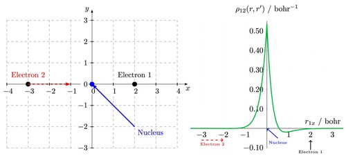15) In order to plot the dynamic Coulomb holes, the inter-particle coordinate system is first transformed into Cartesian coordinates using the following coordinate transformations (16) $\begin{array}{rl}{r}_1& =(r_{1x}^2+r_{1y}^2+r_{1z}^2{)}^{\frac{1}{2}},\\ r_2& =(r_{2x}^2+r_{2y}^2+r_{2z}^2{)}^{\frac{1}{2}},\\ r_{12}& =((r_{1x}-r_{2x}{)}^2+(r_{1y}-r_{2y}{)}^2+(r_{1z}-r_{2z}{)}^2{)}^{\frac{1}{2}}.\end{array}$(16) The nucleus is fixed at the origin with electron 1 fixed on the x-axis at a specified position. Electron 2 is then moved along the x-axis and the two-electron density is calculated point-by-point using Equation (13(13) ${\rho }_{12}(r,r^{\mathrm{\prime }})=\underset{\mathrm{Fermi}\mathrm{Coulomb}\mathrm{hole}}{\underbrace{{\rho }_{xc}(r,r^{\mathrm{\prime }})}}-\underset{\mathrm{Fermi}\mathrm{hole}}{\underbrace{{\rho }_x(r,r^{\mathrm{\prime }})}},$(13) ). An example of a two-electron system represented in the Cartesian space is given in Figure 2.

Figure 2. (left) Cartesian coordinate system used in calculating dynamic Coulomb holes. The nucleus is fixed at the origin, electron 1 is fixed on the positive x axis and electron 2 is moved along the x axis. (right) The resulting dynamic Coulomb hole for the helium atom using the Cartesian schematic on the left.

Equation (13(13) ${\rho }_{12}(r,r^{\mathrm{\prime }})=\underset{\mathrm{Fermi}\mathrm{Coulomb}\mathrm{hole}}{\underbrace{{\rho }_{xc}(r,r^{\mathrm{\prime }})}}-\underset{\mathrm{Fermi}\mathrm{hole}}{\underbrace{{\rho }_x(r,r^{\mathrm{\prime }})}},$(13) ) represents the ‘exact’ dynamic Coulomb hole, i.e. the one in reference to a FC wavefunction.

Moscardó et al. [25] calculated the dynamic Coulomb in the context of the CS methodology using the following form (17) ${\rho }_c({\mathbf{r}}_1,{\mathbf{r}}_2)=\frac{{\mathrm{\Gamma }}_2^0({\mathbf{r}}_1,{\mathbf{r}}_2)[{\varphi }^2({\mathbf{r}}_1,{\mathbf{r}}_2)-2\varphi ({\mathbf{r}}_1,{\mathbf{r}}_2)]}{{\rho }^0({\mathbf{r}}_1)},$(17) where ${\mathrm{\Gamma }}_2^0({\mathbf{r}}_1,{\mathbf{r}}_2)$ is the two-electron density matrix and ${\rho }^0({\mathbf{r}}_1)$ the one-electron density. Moscardó et al. used a value of q = 1.17 within the CS method whereas in this work we use the value reported in the original work q = 2.29 [4]. Equation (17(17) ${\rho }_c({\mathbf{r}}_1,{\mathbf{r}}_2)=\frac{{\mathrm{\Gamma }}_2^0({\mathbf{r}}_1,{\mathbf{r}}_2)[{\varphi }^2({\mathbf{r}}_1,{\mathbf{r}}_2)-2\varphi ({\mathbf{r}}_1,{\mathbf{r}}_2)]}{{\rho }^0({\mathbf{r}}_1)},$(17) ) will be referred to as an ‘approximate’ dynamic Coulomb hole, used to compare against the ‘exact’ dynamic Coulomb holes for different two-electron systems. However, it should be noted that the correlation energy approximated by the CS/LYP functionals use the empirical 4-parameter correlation energy formula (7(7) $E_{\mathrm{corr}}^{\mathrm{CS}}=-\pi \int a\left(\frac{1+bW\exp (-c/\beta )}{1+d/\beta }\right)\rho (\mathbf{R})\mathrm{d}\mathbf{R},$(7) ) whereas here we follow the approach taken in the literature [6,25] and perform our analysis using the CS wavefunction (5(5) $\begin{array}{rl}& {\mathrm{\Psi }}_{\mathrm{CS}}({\mathbf{x}}_1,{\mathbf{x}}_2,\dots ,{\mathbf{x}}_N)\\ & ={\mathrm{\Psi }}_{\mathrm{HF}}({\mathbf{x}}_1,{\mathbf{x}}_2,\dots ,{\mathbf{x}}_N)\prod _{i>j}^{}(1-\varphi ({\mathbf{r}}_i,{\mathbf{r}}_j)),\end{array}$(5) ).

2.3. Radial energy

In analogy to the Coulomb hole, we calculate the energy for 1000 $r_{12}$ values by calculating the expectation value of the energy operator evaluated at a given $r_{12}=r$, i.e. (18) $\begin{array}{rl}{\epsilon }_{\mathrm{FC}}(r)& ={\frac{⟨{\mathrm{\Psi }}^{\mathrm{FC}}|\hat{H}|{\mathrm{\Psi }}^{\mathrm{FC}}⟩}{⟨{\mathrm{\Psi }}^{\mathrm{FC}}|{\mathrm{\Psi }}^{\mathrm{FC}}⟩}|}_{r_{12}=r},\\ {\epsilon }_{\mathrm{HF}}(r)& ={\frac{⟨{\mathrm{\Psi }}^{\mathrm{HF}}|2\hat{F}-\hat{J}|{\mathrm{\Psi }}^{\mathrm{HF}}⟩}{⟨{\mathrm{\Psi }}^{\mathrm{HF}}|{\mathrm{\Psi }}^{\mathrm{HF}}⟩}|}_{r_{12}=r},\end{array}$(18) which provides the energy at discrete points. These energy densities, $\epsilon (r)$, are defined such that (19) $E_{\mathrm{FC}}={\int }_0^{\mathrm{\infty }}{\epsilon }_{\mathrm{FC}}(r)\mathrm{d}r\mathrm{and}{E}_{\mathrm{HF}}={\int }_0^{\mathrm{\infty }}{\epsilon }_{\mathrm{HF}}(r)\mathrm{d}r.$(19) However, there can be ambiguity in the definition of energy densities. For example, it has been shown that there is an inherent ambiguity in the definition of the kinetic energy density, where although the same numerical values of the kinetic energy is obtained, the kinetic energy density, defined to be the contribution to the kinetic energy from a given interval can provide different results [35]. In the present work, ${\epsilon }_{\mathrm{FC}}(r)$ and ${\epsilon }_{\mathrm{HF}}(r)$ are both calculated using the ‘nabla squared’ (${\mathrm{\nabla }}^2$) rather than the ‘del dot del’ ($\mathrm{\nabla }\cdot \mathrm{\nabla }$) definition of the local kinetic energy density. In terms of implementation, the Hamiltonian operator is applied to the optimised wavefunction to get the full integrand, before substituting the $r_{12}=r$ value and integrating over just $r_1$ and $r_2$. To determine the correlation energy densities, we calculate (20) $E_{\mathrm{corr}}={\int }_0^{\mathrm{\infty }}{\epsilon }_{\mathrm{corr}}(r)\mathrm{d}r={\int }_0^{\mathrm{\infty }}\{{\epsilon }_{\mathrm{FC}}(r)-{\epsilon }_{\mathrm{HF}}(r)\}\mathrm{d}r.$(20) In the case of the CS formalism, $E_{\mathrm{corr}}$ is defined in terms of the extracule coordinate R rather than the intracule coordinate $r\equiv r_{12}$. Therefore, we also calculated ${\epsilon }_{\mathrm{FC}}(R)$ and ${\epsilon }_{\mathrm{HF}}(R)$ by evaluating the expectation value of the energy operator at a given R value. The difference between the FC and HF energy densities delivers the correlation energy, i.e. for the helium atom, $E_{\mathrm{corr}}={\int }_0^{\mathrm{\infty }}\{{\epsilon }_{\mathrm{FC}}(R)-{\epsilon }_{\mathrm{HF}}(R)\}\mathrm{d}R={\int }_0^{\mathrm{\infty }}{\epsilon }_{\mathrm{corr}}(R)\mathrm{d}R=-0.042044282$.

To calculate the CS-derived radial energy distributions ${\epsilon }_{\mathrm{corr}}^{\mathrm{CS}}(R)$ and ${\epsilon }_{\mathrm{corr}}^{\mathrm{LYP}}(R)$, we use the open-shell CS and LYP functionals, Equations (9(9) $\begin{array}{rl}{E}_{\text{corr}}^{\text{CS-LYP}}=-a\pi \int & \frac{\gamma (\mathbf{R})}{1+\frac{d}{q}{\rho }^{-1/3}(\mathbf{R})}\{\rho (\mathbf{R})+\frac{8b}{q^2}{\rho }^{-5/3}(\mathbf{R})\\ & [{\rho }_{\alpha }(\mathbf{R})t_{\text{HF}}^{\alpha }+{\rho }_{\beta }(\mathbf{R})t_{\text{HF}}^{\beta }-\rho (\mathbf{R})t_W(\mathbf{R})]\\ & e^{-\frac{c}{q}{\rho }^{-1/3}(\mathbf{R})}\}\text{d}\mathbf{R},\end{array}$(9) ) and (10(10) $\begin{array}{rl}{E}_{\mathrm{corr}}^{\mathrm{LYP}}& =-a\pi \int \frac{\gamma (\mathbf{R})}{1+\frac{d}{q}{\rho }^{-1/3}(\mathbf{R})}\{\rho (\mathbf{R})+\frac{8b}{q^2}{\rho }^{-5/3}(\mathbf{R})\\ & [\phantom{+\frac{1}{18}({\rho }_{\alpha }(\mathbf{R}){\mathrm{\nabla }}^2{\rho }_{\alpha }(\mathbf{R})+{\rho }_{\beta }(\mathbf{R}){\mathrm{\nabla }}^2{\rho }_{\beta }(\mathbf{R}))]{\mathrm{e}}^{-\frac{c}{q}{\rho }^{-1/3}(\mathbf{R})}\}}{2}^{2/3}{C}_F{\rho }_{\alpha }^{8/3}(\mathbf{R})+2^{2/3}{C}_F{\rho }_{\beta }^{8/3}(\mathbf{R})-\rho (\mathbf{R})t_W\\ & +\frac{1}{9}({\rho }_{\alpha }(\mathbf{R})t_W^{\alpha }(\mathbf{R})+{\rho }_{\beta }(\mathbf{R})t_W^{\beta }(\mathbf{R}))\\ & +\frac{1}{18}({\rho }_{\alpha }(\mathbf{R}){\mathrm{\nabla }}^2{\rho }_{\alpha }(\mathbf{R})+{\rho }_{\beta }(\mathbf{R}){\mathrm{\nabla }}^2{\rho }_{\beta }(\mathbf{R}))]\\ & {\mathrm{e}}^{-\frac{c}{q}{\rho }^{-1/3}(\mathbf{R})}\phantom{\frac{1}{18}}\}\mathrm{d}\mathbf{R},\end{array}$(10) ) respectively; their integrands are evaluated for 1000 values of R and plotted. No explicit integration is required owing to a singular dependence on the extracule coordinate, R.

3. Results

3.1. Static Coulomb holes

Static Coulomb holes (SCH) provide a measure of the radial correlation between two electrons where $r_{12}$ is the distance between them. In Figure 3, the intracule distribution functions $D_{\mathrm{FC}}$ and $D_{\mathrm{CS}}$ and the difference between them $D_{\mathrm{FC}}-D_{\mathrm{CS}}$ is plotted for the four systems: Li${}^{+}$, He, H${}^{-}$ and the critical nuclear charge for binding, Z${}_C^{\mathrm{FC}}$. The ‘exact’ static Coulomb holes $D_{\mathrm{FC}}-D_{\mathrm{HF}}$ are also provided [23].

Figure 3. The exact static Coulomb hole curve (solid red line) [23], compared to the difference between the intracule distribution functions $D_{\mathrm{FC}}(r)$ and $D_{\mathrm{CS}}(r)$ (solid orange line). The inset plots in (a,b) reveals the secondary Coulomb holes, and the inset plots in (c,d) show a zoom of the primary Coulomb hole region. (a) Li${}^{+}$ (b) He (c) H${}^{-}$ (d) Z${}_C^{\mathrm{FC}}$

Figure 3 shows that for all systems, the primary static Coulomb hole decreases in size when using the CS wavefunction in place of the HF wavefunction, demonstrating that the Jastrow-style function captures some of the physics of the exact system. The key properties of the intracule difference $D_{\mathrm{FC}}-D_{\mathrm{CS}}$, for each systems, are tabulated in Table 1 and compared with the exact Coulomb hole as a % difference. Using the CS wavefunction in place of the HF wavefunction decreases the area of the hole by $\approx 30\mathrm{\%}$ for He and Li${}^{+}$. However, the positive part of the hole (sometimes called the Coulomb heap) shows virtually no change and the secondary Coulomb holes for He and Li${}^{+}$ remain present. It is not unexpected that a cusp-based approximation behaves more like the HF wavefunction that the FC wavefunction at greater electron-electron separations. As shown previously [23], the probability that the two electrons will be found at large separations reduces more rapidly than when the electronic motions are uncorrelated for $Z\ge 2$ because as Z increases and the electrons are drawn closer to the nucleus the correlated electrons can adjust their relative positions and maximise the attractive interaction. Thus, while the CS wavefunction reduces some of the HF errors at small r corresponding to regions of large electron density, it does not appear to recover the correlation energy at longer range.

3.2. Dynamic Coulomb holes

The dynamic Coulomb hole (DCH) provides information on how the two electrons are correlated as a function of the non-uniform density of the atom. Figure 4 provides the ‘exact’ dynamic Coulomb holes, calculated using (13(13) ${\rho }_{12}(r,r^{\mathrm{\prime }})=\underset{\mathrm{Fermi}\mathrm{Coulomb}\mathrm{hole}}{\underbrace{{\rho }_{xc}(r,r^{\mathrm{\prime }})}}-\underset{\mathrm{Fermi}\mathrm{hole}}{\underbrace{{\rho }_x(r,r^{\mathrm{\prime }})}},$(13) ), for the lithium cation, the helium atom and the hydride ion, with an electron at three key points (i) the most probable nucleus electron distance $r_{max}$ (top row), (ii) the surface region of the atom which we have taken to be the point at which the static Coulomb hole becomes positive, i.e. the first non-zero root ${\mathrm{\Delta }}_1^{root}$ (middle row), and (iii) at a distance of 2 $a_0$ (bottom row), which for Li${}^{+}$ and He is the region where Coulomb correlation increases the probability that the electrons are separated by given distance r compared to when Coulomb correlations are absent; for the hydride ion, this distance corresponds to $r<{\mathrm{\Delta }}_1^{root}$ in which the Coulomb correlation reduces the probability of the two electrons being a certain distance apart and the static Coulomb hole is negative. The values of ${\mathrm{\Delta }}_1^{root}$ are provided in Table 1 in parentheses and $r_{max}$ = 0.362 873 $a_0$ for Li${}^{+}$, 0.566 087 $a_0$ for He, 1.176 970 $a_0$ for H${}^{-}$ ion and 1.232 272 $a_0$ for the Z${}_C^{\mathrm{FC}}$ system. The dynamic Coulomb holes for $Z_C^{\mathrm{FC}}$ and $Z_C^{\mathrm{HF}}$ have a very similar structure to the hydride ion and so are not shown.

Figure 4. The dynamic Coulomb holes for Li${}^{+}$ (left), He (center), and H${}^{-}$ (right); note the different y-axis scales. The nucleus is at the origin, electron 1 is fixed on the positive x axis (indicated by an arrow). Top row corresponds to electron 1 at the most probable distance from the nucleus $r_{max}$, middle row corresponds to the crossing point in the static Coulomb hole ${\mathrm{\Delta }}_1^{root}$, and row 3 corresponds to electron 1 at 2 $a_0$.

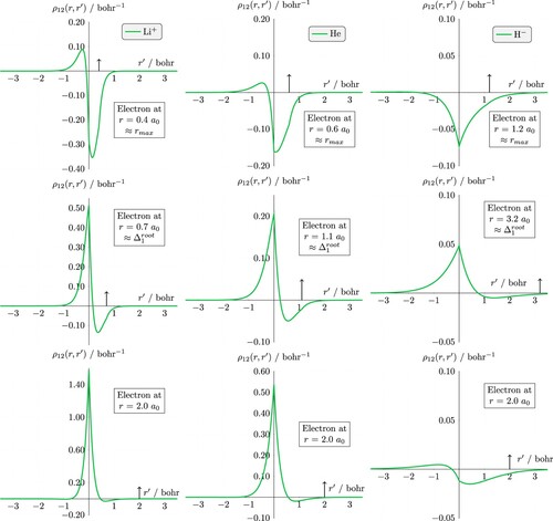
Table 1. Roots, areas and minima of the $D_{\mathrm{FC}}-D_{\mathrm{CS}}$ curves in the helium-like ions in atomic units.

system	${\mathrm{\Delta }}_1^{min}$	${\mathrm{\Delta }}_1^{root}$	${\mathrm{\Delta }}_2^{min}$	${\mathrm{\Delta }}_2^{root}$	${\mathrm{\Delta }}_1^{area}$	${\mathrm{\Delta }}_2^{area}$
Z${}_C^{\mathrm{FC}}$	2.02 (1.91, 5.8%)	4.87 (4.85, 0.4%)	–	–	2.08$\times {10}^{-1}$ (2.39$\times {10}^{-1}$ , −9.6%)	–
H${}^{-}$	1.58 (1.46, 8.2%)	3.21 (3.20, 0.3%)	–	–	1.12$\times {10}^{-1}$ (1.33$\times {10}^{-1}$, −15.8%)	–
He	0.59 (0.52, 13.5%)	1.07 (1.07, 0%)	4.08 (4.08, 0%)	3.56 (3.58, −0.6%)	3.26$\times {10}^{-2}$ (4.63$\times {10}^{-2}$, −29.6%)	6.28$\times {10}^{-4}$ (6.12$\times {10}^{-4}$, 2.6%)
Li${}^{+}$	0.37 (0.32, 15.6%)	0.66 (0.66, 0%)	2.50 (2.51, −0.4%)	2.19 (2.21, −0.9%)	1.99$\times {10}^{-2}$ (2.80$\times {10}^{-2}$, −28.9%)	3.63$\times {10}^{-4}$ (3.50$\times {10}^{-4}$, 3.7%)

Notes: ${\mathrm{\Delta }}_1$ and ${\mathrm{\Delta }}_2$ refer to the primary and secondary Coulomb holes, respectively. Numbers in brackets are the Coulomb hole values using a HF reference [23] and the percentage difference between using CS and HF as reference.

All dynamic Coulomb holes exhibit a cusp at the position of the fixed electron and the structure of the Coulomb holes is qualitatively similar. When electron 1 is positioned at the most probable nucleus-electron distance, the hole at the electron is negative, as expected, demonstrating the reduced probability of the electrons being separated by these distances. However, on the other side of the nucleus, there is a small positive part indicating that the other electron is more likely to be found in this region, in agreement with previous findings for He [5]. However, for the hydride ion (and the $Z_C$ systems not shown) this positive region is very small when the fixed electron is at $r_{max}$ and only becomes clearly evident as electron 1 is moved further from the nucleus, see plot when $r=2a_0$. Figure 4 also shows that the Coulomb hole, both the negative part in the region of the fixed electron and the positive part on the other side of the nucleus, increases with increasing Z as the correlated electrons adjust their relative positions to maximise the increasing nucleus-electron attraction [23,36]. As the distance of electron 1 from the nucleus increases, the magnitude of the positive part of the hole increases relative to the negative part about electron 1 and moves closer to the nucleus. At the surface of the atom, the positive part of the hole is very close to the nucleus Figure 4 (middle Row) and as electron 1 moves to the outer region of the atom, the positive part of the hole becomes increasingly centred about the nucleus and the negative part diminishes. At large r, when one of the electrons is in the asymptotic region, the second electron is localised about the nucleus.

Singh et al. [6] provided a critical analysis of the CS wavefunction functional of the density and reported that as the electron position is moved from inside the atom at $r_{max}$, to the surface region, the CS Coulomb hole becomes progressively worse. Here we extend that analysis to the lithium cation and the hydrogen anion, as shown in Figure 5. The dynamic Coulomb hole is calculated using (13(13) ${\rho }_{12}(r,r^{\mathrm{\prime }})=\underset{\mathrm{Fermi}\mathrm{Coulomb}\mathrm{hole}}{\underbrace{{\rho }_{xc}(r,r^{\mathrm{\prime }})}}-\underset{\mathrm{Fermi}\mathrm{hole}}{\underbrace{{\rho }_x(r,r^{\mathrm{\prime }})}},$(13) ) for the exact Coulomb hole [5] and using (17(17) ${\rho }_c({\mathbf{r}}_1,{\mathbf{r}}_2)=\frac{{\mathrm{\Gamma }}_2^0({\mathbf{r}}_1,{\mathbf{r}}_2)[{\varphi }^2({\mathbf{r}}_1,{\mathbf{r}}_2)-2\varphi ({\mathbf{r}}_1,{\mathbf{r}}_2)]}{{\rho }^0({\mathbf{r}}_1)},$(17) ) for the approximate Coulomb hole derived using the CS methodology [25], as a function of the positions of electron 1 and electron 2. For each system, the dynamic Coulomb hole where electron 1 is fixed at the most probable position of the radial distribution function $r_{max}$ for that system has been marked as the dark orange dashed line. Figure 5 also provides a comparison between the exact Coulomb hole (left) and the approximate CS Coulomb hole (right) for the lithium cation, Li${}^{+}$, the helium atom, He, and the hydride ion, H${}^{-}$. It is clear that the CS dynamic Coulomb holes fail to capture the magnitude and sharp features of the exact hole and that the electron-electron cusp is too weak to be observed in the CS Coulomb hole; the discrepancy increases as the nuclear charge is decreased.

Figure 5. (Left) exact DCH using (13(13) ${\rho }_{12}(r,r^{\mathrm{\prime }})=\underset{\mathrm{Fermi}\mathrm{Coulomb}\mathrm{hole}}{\underbrace{{\rho }_{xc}(r,r^{\mathrm{\prime }})}}-\underset{\mathrm{Fermi}\mathrm{hole}}{\underbrace{{\rho }_x(r,r^{\mathrm{\prime }})}},$(13) ) and (right) approximate DCH using (17(17) ${\rho }_c({\mathbf{r}}_1,{\mathbf{r}}_2)=\frac{{\mathrm{\Gamma }}_2^0({\mathbf{r}}_1,{\mathbf{r}}_2)[{\varphi }^2({\mathbf{r}}_1,{\mathbf{r}}_2)-2\varphi ({\mathbf{r}}_1,{\mathbf{r}}_2)]}{{\rho }^0({\mathbf{r}}_1)},$(17) ) for Li${}^{+}$, He and H${}^{-}$. The position of electron 1 is indicated by the circles along the base of each plot. The orange dashed line represents the dynamic Coulomb hole when electron 1 is at $r_{max}$.

3.3. Electron correlation energies and radial energy distributions

The electronic correlation energy, as defined by Lowdin (1(1) $E_{\mathrm{corr}}=E_{\mathrm{exact}}-E_{\mathrm{HF}}.$(1) ), is essentially a measure of the error in the HF method [136]; $E_{\mathrm{HF}}$ is an upper bound to the exact energy E and so the correlation energy is negative. 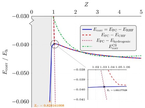Previously, we presented the correlation energies for the helium isoelectronic sequence Z = 1−18 along with the correlation energy at $Z_C^{\mathrm{FC}}$, the nuclear charge just prior to electron detachment [16]. The correlation energy as a fraction of the total energy increases monotonically as Z decreases, as expected. The importance of electron correlation to the stability of anions is well documented. However, the correlation energies do not decrease monotonically and exhibit a maximum (smallest magnitude) as can be seen in Figure 6 (blue solid line), and this is explored further here. It is found that the smallest correlation energy occurs at $Z\approx 1.08$, in fact the $\mathrm{\Delta }{E}_{\mathrm{corr}}\le 8\times {10}^{-5}$ a.u. = 0.2 kJmol${}^{-1}$ for $1.02\le Z\le 1.15$. This range contains our previous estimate of $Z_C^{\mathrm{HF}}=1.031177528$ which corresponds to a correlation energy, $E_{corr}=0.0397151174$ hartree [16]. The shaded area of Figure 6 corresponds to values below the critical nuclear charge for binding in the fully-correlated system, i.e. for $Z_C^{\mathrm{FC}}$. Also, shown by the orange cross is the correlation energy determined at $Z_C^{{\mathrm{HF}}_0}=0.828161008$, the point at which the occupied orbital energy becomes zero [17]. On physical grounds, using RHF to determine $E_{\mathrm{HF}}$ is a poor approximation for weakly bound anions, and it is known that H${}^{-}$ at the RHF level of theory does not hold a bound state [11]. As seen in the inset of Figure 6, energies calculated using RHF and UHF are equal to $\sim m{E}_h$ for $Z\ge 1.05$, but the broken-symmetry solution of UHF results in a divergence in calculated correlation energies below this charge value, where the UHF energy approaches the hydrogenic energy and thus aligns with the $E_{\mathrm{FC}}-E_{\mathrm{hydrogenic}}$ line. This charge value of 1.05 is in good agreement with the very accurate UHF symmetry-breaking threshold, $Z_{sb}^{\mathrm{UHF}}=1.0576602534$ [17]. It is also shown in Figure 6 that the electron correlation energies calculated using the CS formula, Equation (7(7) $E_{\mathrm{corr}}^{\mathrm{CS}}=-\pi \int a\left(\frac{1+bW\exp (-c/\beta )}{1+d/\beta }\right)\rho (\mathbf{R})\mathrm{d}\mathbf{R},$(7) ), decrease smoothly and are greatly underestimated in the range $1\le Z\le 2$. The CS formula was fitted to the helium atom, hence the longer-range, more weakly bound behaviour found at lower nuclear charges is not well described [9].

Figure 6. Electron correlation energies as a function of nuclear charge Z. The black cross corresponds to $Z_C^{\mathrm{HF}}=1.031177528$ and the orange cross corresponds to $Z_C^{{\mathrm{HF}}_0}=0.828161008$. The grey shaded region represents unbound systems, i.e. with $Z\le 0.910$ [15,37]. The inset provides a zoomed view near the maximum in $E_{\mathrm{corr}}$.

In analogy to the Coulomb hole (11(11) $\mathrm{\Delta }D(r)=D_{\mathrm{FC}}(r)-D_{\mathrm{HF}}(r)$(11) ), we now consider the correlation energy radial distributions (energy densities) by calculating ${\epsilon }_{\mathrm{FC}}(r)$ and ${\epsilon }_{\mathrm{HF}}(r)$, for a range of inter-electronic $r_{12}=r$ values, and calculating ${\epsilon }_{\mathrm{corr}}(r)={\epsilon }_{\mathrm{FC}}(r)-{\epsilon }_{\mathrm{HF}}(r)$, i.e. the ‘energy hole’. These values are defined such that $E_{\mathrm{FC}}={\int }_0^{\mathrm{\infty }}{\epsilon }_{\mathrm{FC}}(r)\mathrm{d}r$, $E_{\mathrm{HF}}={\int }_0^{\mathrm{\infty }}{\epsilon }_{\mathrm{HF}}(r)\mathrm{d}r$ and $E_{\mathrm{corr}}={\int }_0^{\mathrm{\infty }}{\epsilon }_{\mathrm{corr}}(r)\mathrm{d}r$ and plotted in Figure 7 for the lithium cation, helium atom, hydride ion and critical nuclear charge system, $Z_C^{\mathrm{FC}}$.

Figure 7. FC and HF radial (intracule) energies, ${\epsilon }^{\mathrm{FC}}(r)$, ${\epsilon }^{\mathrm{HF}}(r)$ for Li${}^{+}$, He, H${}^{-}$ and $Z_C^{\mathrm{FC}}$. The difference between these two curves (shaded region) represents the electron correlation energy distribution, ${\epsilon }_{\mathrm{corr}}(r)$, where ${\int }_0^{\mathrm{\infty }}{\epsilon }_{\mathrm{corr}}(r)\mathrm{d}r=E_{\mathrm{corr}}$. (a) Li${}^{+}$ (b) He (c) H${}^{-}$ (d) Z${}_C^{\mathrm{FC}}$.

Figure 7 shows that ${\epsilon }_{\mathrm{FC}}$, taken as the exact energy radial distribution (blue dashed line), is negative for all electron-electron separations. However, the HF energy radial distribution (red dotted line) is positive for small values of r for all systems tested. As the nuclear charge decreases from Li${}^{+}$ to $Z_C^{\mathrm{FC}}$ the area of the positive energy region in the HF energy curve increases; this we attribute to the contribution of the kinetic energy term to the total energy becoming more dominant with decreasing nuclear charge.

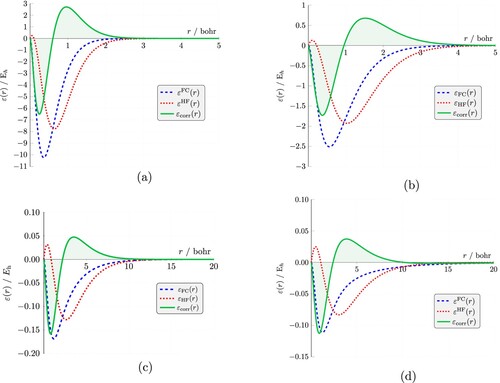
The electron correlation energy, $E_{\mathrm{corr}}$ is by definition negative, but it is clear from Figure 7 that regions of coordinate space exist where it is positive. However, the negative part of the energy hole lies at $r_{12}\equiv r$ values within the surface region of the atom, defined earlier as ${\mathrm{\Delta }}_1^{root}$ of the Coulomb hole, i.e. the region in which Coulomb correlations reduce the probability of two electrons being a certain distance apart.

The question arises, how does the energy density using the CS/LYP method compare with the ‘exact’ energy density hole? To answer this question we first need to calculate the ‘exact’ correlation energy distributions as a function of the extracule coordinate R, i.e. ${\epsilon }_{\mathrm{corr}}(R)={\epsilon }_{\mathrm{FC}}(R)-{\epsilon }_{\mathrm{HF}}(R)$ and then compare with ${\epsilon }_{\mathrm{corr}}^{\mathrm{CS}}(R)$ calculated using (9(9) $\begin{array}{rl}{E}_{\text{corr}}^{\text{CS-LYP}}=-a\pi \int & \frac{\gamma (\mathbf{R})}{1+\frac{d}{q}{\rho }^{-1/3}(\mathbf{R})}\{\rho (\mathbf{R})+\frac{8b}{q^2}{\rho }^{-5/3}(\mathbf{R})\\ & [{\rho }_{\alpha }(\mathbf{R})t_{\text{HF}}^{\alpha }+{\rho }_{\beta }(\mathbf{R})t_{\text{HF}}^{\beta }-\rho (\mathbf{R})t_W(\mathbf{R})]\\ & e^{-\frac{c}{q}{\rho }^{-1/3}(\mathbf{R})}\}\text{d}\mathbf{R},\end{array}$(9) ) which is equivalent to (7(7) $E_{\mathrm{corr}}^{\mathrm{CS}}=-\pi \int a\left(\frac{1+bW\exp (-c/\beta )}{1+d/\beta }\right)\rho (\mathbf{R})\mathrm{d}\mathbf{R},$(7) ) for a closed-shell system, where ${\int }_0^{\mathrm{\infty }}{\epsilon }_{\mathrm{corr}}^{\mathrm{CS}}(R)\mathrm{d}R=E_{\mathrm{corr}}^{\mathrm{CS}-\mathrm{LYP}}\equiv E_{\mathrm{corr}}^{\mathrm{CS}}$. Figure 8(a) shows the FC and HF radial energy distributions for the helium atom. As a function of the extracule coordinate (the distance from the nucleus to the centre-of-mass of the electron pair) the depth of the well is much deeper and the shape of the FC and HF curves are very similar. Figure 8(a) also reveals that there is no erroneous positive region in the HF distribution. However the difference in the distributions, i.e. ${\epsilon }_{\mathrm{FC}}(R)-{\epsilon }_{\mathrm{HF}}(R)={\epsilon }_{\mathrm{corr}}(R)$ shows both positive and negative R value regions.

Figure 8. (a) The FC and HF radial (extracule) energies, ${\epsilon }^{\mathrm{FC}}(R)$, ${\epsilon }^{\mathrm{HF}}(R)$ and electron correlation energy distribution, ${\epsilon }_{\mathrm{corr}}(R)$, and (b) comparison of ${\epsilon }_{\mathrm{corr}}(R)$ with $E_{\mathrm{corr}}^{CS}(R)$ calculated using Equation (9(9) $\begin{array}{rl}{E}_{\text{corr}}^{\text{CS-LYP}}=-a\pi \int & \frac{\gamma (\mathbf{R})}{1+\frac{d}{q}{\rho }^{-1/3}(\mathbf{R})}\{\rho (\mathbf{R})+\frac{8b}{q^2}{\rho }^{-5/3}(\mathbf{R})\\ & [{\rho }_{\alpha }(\mathbf{R})t_{\text{HF}}^{\alpha }+{\rho }_{\beta }(\mathbf{R})t_{\text{HF}}^{\beta }-\rho (\mathbf{R})t_W(\mathbf{R})]\\ & e^{-\frac{c}{q}{\rho }^{-1/3}(\mathbf{R})}\}\text{d}\mathbf{R},\end{array}$(9) ). All data are for the helium atom.

Figure 8(b) provides a comparison between the ‘exact’ correlation energy radial distribution and the CS distribution calculated using Equation (9(9) $\begin{array}{rl}{E}_{\text{corr}}^{\text{CS-LYP}}=-a\pi \int & \frac{\gamma (\mathbf{R})}{1+\frac{d}{q}{\rho }^{-1/3}(\mathbf{R})}\{\rho (\mathbf{R})+\frac{8b}{q^2}{\rho }^{-5/3}(\mathbf{R})\\ & [{\rho }_{\alpha }(\mathbf{R})t_{\text{HF}}^{\alpha }+{\rho }_{\beta }(\mathbf{R})t_{\text{HF}}^{\beta }-\rho (\mathbf{R})t_W(\mathbf{R})]\\ & e^{-\frac{c}{q}{\rho }^{-1/3}(\mathbf{R})}\}\text{d}\mathbf{R},\end{array}$(9) ). The CS distribution, ${\epsilon }_{\mathrm{corr}}^{\mathrm{CS}}(R)$ does not resemble ${\epsilon }_{\mathrm{corr}}(R)$ at all. In particular, ${\epsilon }_{\mathrm{corr}}^{\mathrm{CS}}(R)$ is negative for all R except in the small interval R<0.055 where it takes on slightly positive values. This finding is in agreement with Caratzoulas and Knowles [7].

To explore this further, we calculate the radial energy distributions for atoms (Li, O), anions (B${}^{-}$, F${}^{-}$) and cations (C${}^{+}$, N${}^{+}$) using the approximate open-shell CS and LYP expressions for calculating the electron correlation energy, Equations (9(9) $\begin{array}{rl}{E}_{\text{corr}}^{\text{CS-LYP}}=-a\pi \int & \frac{\gamma (\mathbf{R})}{1+\frac{d}{q}{\rho }^{-1/3}(\mathbf{R})}\{\rho (\mathbf{R})+\frac{8b}{q^2}{\rho }^{-5/3}(\mathbf{R})\\ & [{\rho }_{\alpha }(\mathbf{R})t_{\text{HF}}^{\alpha }+{\rho }_{\beta }(\mathbf{R})t_{\text{HF}}^{\beta }-\rho (\mathbf{R})t_W(\mathbf{R})]\\ & e^{-\frac{c}{q}{\rho }^{-1/3}(\mathbf{R})}\}\text{d}\mathbf{R},\end{array}$(9) ) and (10(10) $\begin{array}{rl}{E}_{\mathrm{corr}}^{\mathrm{LYP}}& =-a\pi \int \frac{\gamma (\mathbf{R})}{1+\frac{d}{q}{\rho }^{-1/3}(\mathbf{R})}\{\rho (\mathbf{R})+\frac{8b}{q^2}{\rho }^{-5/3}(\mathbf{R})\\ & [\phantom{+\frac{1}{18}({\rho }_{\alpha }(\mathbf{R}){\mathrm{\nabla }}^2{\rho }_{\alpha }(\mathbf{R})+{\rho }_{\beta }(\mathbf{R}){\mathrm{\nabla }}^2{\rho }_{\beta }(\mathbf{R}))]{\mathrm{e}}^{-\frac{c}{q}{\rho }^{-1/3}(\mathbf{R})}\}}{2}^{2/3}{C}_F{\rho }_{\alpha }^{8/3}(\mathbf{R})+2^{2/3}{C}_F{\rho }_{\beta }^{8/3}(\mathbf{R})-\rho (\mathbf{R})t_W\\ & +\frac{1}{9}({\rho }_{\alpha }(\mathbf{R})t_W^{\alpha }(\mathbf{R})+{\rho }_{\beta }(\mathbf{R})t_W^{\beta }(\mathbf{R}))\\ & +\frac{1}{18}({\rho }_{\alpha }(\mathbf{R}){\mathrm{\nabla }}^2{\rho }_{\alpha }(\mathbf{R})+{\rho }_{\beta }(\mathbf{R}){\mathrm{\nabla }}^2{\rho }_{\beta }(\mathbf{R}))]\\ & {\mathrm{e}}^{-\frac{c}{q}{\rho }^{-1/3}(\mathbf{R})}\phantom{\frac{1}{18}}\}\mathrm{d}\mathbf{R},\end{array}$(10) ) respectively. The HF wavefunctions from Koga et al. [38] were used for these many-electron systems. Figure 9 shows that for all systems both the CS and LYP functionals exhibit a small positive region at small R. The origin of this small positive region is not clear, nor whether it holds any significance given that the exact energy hole as a function of R also has a positive region at small R values, close to the nucleus.

Figure 9. Radial electron correlation energy distributions, $E_{\mathrm{corr}}(R)$, calculated using (a) the CS open-shell energy formula (9(9) $\begin{array}{rl}{E}_{\text{corr}}^{\text{CS-LYP}}=-a\pi \int & \frac{\gamma (\mathbf{R})}{1+\frac{d}{q}{\rho }^{-1/3}(\mathbf{R})}\{\rho (\mathbf{R})+\frac{8b}{q^2}{\rho }^{-5/3}(\mathbf{R})\\ & [{\rho }_{\alpha }(\mathbf{R})t_{\text{HF}}^{\alpha }+{\rho }_{\beta }(\mathbf{R})t_{\text{HF}}^{\beta }-\rho (\mathbf{R})t_W(\mathbf{R})]\\ & e^{-\frac{c}{q}{\rho }^{-1/3}(\mathbf{R})}\}\text{d}\mathbf{R},\end{array}$(9) ) and (b) the LYP functional (10(10) $\begin{array}{rl}{E}_{\mathrm{corr}}^{\mathrm{LYP}}& =-a\pi \int \frac{\gamma (\mathbf{R})}{1+\frac{d}{q}{\rho }^{-1/3}(\mathbf{R})}\{\rho (\mathbf{R})+\frac{8b}{q^2}{\rho }^{-5/3}(\mathbf{R})\\ & [\phantom{+\frac{1}{18}({\rho }_{\alpha }(\mathbf{R}){\mathrm{\nabla }}^2{\rho }_{\alpha }(\mathbf{R})+{\rho }_{\beta }(\mathbf{R}){\mathrm{\nabla }}^2{\rho }_{\beta }(\mathbf{R}))]{\mathrm{e}}^{-\frac{c}{q}{\rho }^{-1/3}(\mathbf{R})}\}}{2}^{2/3}{C}_F{\rho }_{\alpha }^{8/3}(\mathbf{R})+2^{2/3}{C}_F{\rho }_{\beta }^{8/3}(\mathbf{R})-\rho (\mathbf{R})t_W\\ & +\frac{1}{9}({\rho }_{\alpha }(\mathbf{R})t_W^{\alpha }(\mathbf{R})+{\rho }_{\beta }(\mathbf{R})t_W^{\beta }(\mathbf{R}))\\ & +\frac{1}{18}({\rho }_{\alpha }(\mathbf{R}){\mathrm{\nabla }}^2{\rho }_{\alpha }(\mathbf{R})+{\rho }_{\beta }(\mathbf{R}){\mathrm{\nabla }}^2{\rho }_{\beta }(\mathbf{R}))]\\ & {\mathrm{e}}^{-\frac{c}{q}{\rho }^{-1/3}(\mathbf{R})}\phantom{\frac{1}{18}}\}\mathrm{d}\mathbf{R},\end{array}$(10) ), for anionic (B${}^{-}$, F${}^{-}$), neutral (Li, O) and cationic (C${}^{+}$, N${}^{+}$) atoms. The inset plots show a zoomed view near the origin, highlighting the small positive regions. (a) CS (b) LYP.

3.4. Expectation values

Various expectation values are provided in Table 2. The electron-electron cusp condition is forced in the CS method [4,8] and thus when using the CS wavefunction a numerically exact electron-electron cusp value is calculated for all systems. The one-electron cusps also show excellent agreement with the exact values for all systems tested. Using the CS wavefunction results in a noticeable improvement when compared to the FC results in the calculated value of $⟨\delta (r_{12})⟩$. In the case of the helium atom, the HF value of $⟨\delta (r_{12})⟩=0.190603997806$ is approximately 79% in error compared to the FC value of 0.106 345. Using the CS wavefunction results in a value of $⟨\delta (r_{12})⟩=0.116862484$ reducing the error to ≈ 9%. Surprisingly, the values of $⟨r_{12}⟩$ calculated using the CS wavefunction are not as accurate as those calculated using the HF wavefunction. This suggests that the CS wavefunction better describes the probability of electron-electron coalescence but does not accurately describe the physical distance, $r_{12}$, itself. This is further highlighted by the fact that the electron-electron cusp is forced in the CS method and the form used to calculate cusps, i.e. ${\nu }_{ij}=\frac{⟨\delta (r_{ij})(\mathrm{\partial }/\mathrm{\partial }{r}_{ij})⟩}{⟨\delta (r_{ij})⟩},$ explicitly depends on the value of $⟨\delta (r_{12})⟩$. Forcing the cusp condition allows for a better description of $⟨\delta (r_{12})⟩$. A noticeable improvement is also seen in the calculated value of $⟨1/r_{12}⟩$ which is a key component of the potential energy operator in the Hamiltonian operator. In the case of the helium atom the error in $⟨1/r_{12}⟩$, compared to the FC value, is approximately halved (from 8% to 4%) when replacing the HF wavefunction with the CS wavefunction. When comparing expectation values involving the nucleus-electron distance, the CS derived values are comparable to HF or slightly worse. This shows that for the systems tested, the CS wavefunction better describes the electron-electron coalescence properties at the expense of a less accurate description of nucleus-electron interactions.

Table 2. Inter-particle expectation values in atomic units, nucleus-electron cusp ${\nu }_{31}$ (exact value $=-Z$) and electron-electron cusp ${\nu }_{12}$ (exact value $=0.5$), for $Z_C^{\mathrm{FC}}$, H${}^{-}$, He and Li${}^{+}$ using either the fully-correlated (FC), Hartree-Fock (HF) or Colle-Salvetti (CS) wavefunctions.

	Z${{}_{\mathbf{C}}}^{\mathrm{FC}}=0.911028224$			H${}^{-}$
Property	FC	HF	CS	FC	HF	CS
〈r1〉	4.146	2.989 00	2.924 668 660	2.710 178 278	2.503 959	2.452 502 536
〈r12〉	7.083	4.493 9	4.483 972 863	4.412 694 49	3.739 273	3.730 877 063
〈δ(r1)〉	0.119 094	0.108 4	0.108 370 481	0.164 552 8	0.154	0.154 432 600
〈δ(r12)〉	0.001 114	0.008 601 2	0.002 932 080	0.002 738	0.012 983 476 3	0.004 870 980
〈1/r1〉	0.578 108	0.595 799 1	0.587 185 657	0.683 261 767 65	0.685 672 15	0.676 064 953
〈1/r12〉	0.223 374	0.337 767	0.313 387 449	0.311 021 502 2	0.395 484 84	0.368 658 025
${\nu }_{31}$	−0.911 0	−0.911 1	−0.911 058 578	−0.999 999 91	−1.000 04	−1.000 005
${\nu }_{12}$	0.499 4	n/a	0.5	0.499 98	n/a	0.5
	He			Li${}^{+}$
	FC	HF	CS	FC	HF	CS
〈r1〉	0.929 472 294 87	0.927 273 404 7	0.914 050 347	0.572 774 149 97	0.572 366 815 001	0.566 098 399
〈r12〉	1.422 070 255 56	1.362 124 383 6	1.358 856 514	0.862 315 375 4	0.838 314 780 311	0.836 578 885
〈δ(r1)〉	1.810 429	1.797 959	1.795 389 539	6.852 00	6.836 07	6.828 714 314
〈δ(r12)〉	0.106 345	0.190 603 997 806	0.116 862 484	0.533 72	0.770 240 340 922	0.555 670 985
〈1/r1〉	1.688 316 800 71	1.687 282 215 281	1.671 771 326	2.687 924 397	2.687 419 466 644	2.669 333 872
〈1/r12〉	0.945 818 448	1.025 768 869	0.983 541 121	1.567 719 559 1	1.651 686 396 960	1.602 611 500
${\nu }_{31}$	−1.999 996	−1.999 999 4	−1.999 999 8	−2.999 999 1	−2.999 999 2	−2.999 999 96
${\nu }_{12}$	0.499 95	n/a	0.5	0.499 998	n/a	0.5

Note: FC and HF values taken from our previous work [23].

4. Conclusions

In this paper we have investigated Coulomb correlation effects in the lithium cation, the helium atom, the hydride ion and the anionic system with the critical nuclear charge for binding by studying the static and dynamic Coulomb holes, the electron correlation energy, the correlation energy densities and the radial correlation energy hole.

The structure of the dynamic Coulomb hole as a function of electron position is qualitatively similar for the systems considered. The Coulomb hole is negative about the fixed electron, indicating the reduction of two-electron density about it due to Coulomb repulsion, and on the other side of the nucleus a positive part of the Coulomb hole gives the positional probability of the other electron which is more pronounced the greater the nuclear charge. In agreement with previous work on the helium atom [5,6,25] it was shown that the CS dynamic Coulomb hole gets progressively worse as the fixed electron is moved to outer regions of the atom and key features such as the cusps are too weak to discern. The static Coulomb hole, calculated as the difference between the FC and the CS intracule densities decreases the size of the primary Coulomb hole for all systems tested when compared to static Coulomb holes calculated with a HF reference wavefunction. However, the secondary Coulomb hole, for Li${}^{+}$ and He, remain reaffirming that the CS wavefunction does not capture the physics at larger r.

High accuracy electron correlation energies were presented using both the RHF and UHF energy as a reference. A maximum in the electron correlation energy is shown at $Z\approx 1.08$, which is just greater than the UHF symmetry-breaking threshold of $\approx 1.05$ which occurs before the minimum charge for which the RHF method can hold a bound state, i.e. $Z_C^{\mathrm{HF}}\approx 1.031$. However, in the region of this maximum the correlation energy is essentially flat.

The correlation energy distributions have been calculated as both a function of the intracule coordinate r and the extracule coordinate R. Both distribution functions have positive and negative regions highlighting that, although the electron correlation energy $E_{\mathrm{corr}}$ is always negative, there exists discrete points in space where it is positive. The shape of the ‘energy hole’ calculated by plotting ${\epsilon }_{\mathrm{corr}}(r)$ is not dissimilar to that of the static Coulomb hole, and it was found that the hole deepens as the nuclear charge increases. However, it was also found that the HF energy densities are positive at small r suggesting that the contribution from the kinetic energy term in HF theory is dominant in this region of space. The ‘exact’ correlation energy densities, ${\epsilon }_{\mathrm{corr}}(R)$, were calculated to provide a direct comparison with the CS distribution ${\epsilon }_{\mathrm{corr}}^{\mathrm{CS}}(R)$ calculated using the CS and LYP correlation energy functional. It was found that the CS distribution ${\epsilon }_{\mathrm{corr}}^{CS}(R)$ does not resemble ${\epsilon }_{\mathrm{corr}}(R)$. It was also shown that ${\epsilon }_{\mathrm{corr}}^{\mathrm{CS}}(R)$ is negative for all R except at very small R where it takes on slightly positive values, a feature that persists for the many electron systems considered.

Data availability statement

The wavefunctions for each system (Li+, He, H- and ZC), along with all the particle density, energy density data, and correlation energy data presented in the paper, are available at http://dx.doi.org/10.25377/sussex.21566013.

Disclosure statement

No potential conflict of interest was reported by the author(s).

Additional information

Funding

H.C. and A.L.B. would like to thank http://dx.doi.org/10.13039/501100000266 Engineering and Physical Sciences Research Council (EPSRC) for financial support [grant number EP/R011265/1] and NVIDIA for providing a Titan V GPU as part of their accelerated data science program. The authors would also like to thank the Royal Society of Chemistry (RSC) for the award of an RSC Summer Research Bursary to P.U.C.

References

- P.O. Löwdin, Int. J. Quantum Chem. 55, 77–102 (1995). doi:10.1002/qua.560550203
- P.O. Löwdin, Phys. Rev. 97, 1509–1520 (1955). doi:10.1103/PhysRev.97.1509
- C. Lee, W. Yang and R. Parr, Phys. Rev. B 37, 785–789 (1988). doi:10.1103/PhysRevB.37.785
- R. Colle and O. Salvetti, Theor. Chim. Acta. 37, 329–334 (1975). doi:10.1007/BF01028401
- M. Slamet and V. Sahni, Phys. Rev. A 51, 2815–2825 (1995). doi:10.1103/PhysRevA.51.2815
- R. Singh, L. Massa and V. Sahni, Phys. Rev. A 60, 4135–4139 (1999). doi:10.1103/PhysRevA.60.4135
- S. Caratzoulas and P.J. Knowles, Mol. Phys. 98, 1811–1821 (2000). doi:10.1080/00268970009483385
- N.C. Handy, Theor. Chem. Acc. 123 (3), 165–169 (2009). doi:10.1007/s00214-009-0522-3
- A.L. Baskerville, M. Targema and H. Cox, R. Soc. Open Sci. 9 (1), 211333 (2022). doi:10.1098/rsos.211333
- C. Hättig, W. Klopper, A. Köhn and D.P. Tew, Chem. Rev. 112 (1), 4–74 (2012). PMID: 22206503. doi:10.1021/cr200168z
- H. Cox, A.L. Baskerville, J.J. Syrjanen and M. Melgaard, Adv. Quantum Chem. 81, 167–189 (2020). doi:10.1016/bs.aiq.2020.04.002
- R.N. Hill, Phys. Rev. Lett. 38, 643–646 (1977). doi:10.1103/PhysRevLett.38.643
- J.D. Baker, D.E. Freund, R.N. Hill and J.D. Morgan, Phys. Rev. A 41, 1247–1273 (1990). doi:10.1103/PhysRevA.41.1247
- C. Estienne, M. Busuttil, A. Moini and G.W.F. Drake, Phys. Rev. Lett. 112, 173001–1–173001–5 (2014). doi:10.1103/PhysRevLett.112.173001
- A.W. King, L. Rhodes, C. Readman and H. Cox, Phys. Rev. A 91, 042512–1–042512–6 (2015). doi:10.1103/PhysRevA.91.042512.
- A.W. King, A.L. Baskerville and H. Cox, Phil. Trans. Soc. A 376, 20170153–1–20170153–16 (2018). doi:10.1098/rsta.2017.0153.
- H.G.A. Burton, J. Chem. Phys. 154 (11), 111103 (2021). doi:10.1063/5.0043105
- H.E. Montgomery Jr., K.D. Sen and J. Katriel, Chem. Phys. Lett. 782, 139030 (2021) https://doi.org/10.1016/j.cplett.2021.139030.
- R.F. Curl and C.A. Coulson, Proc. Phys. Soc. 85 (4), 647 (1965). doi:10.1088/0370-1328/85/4/303
- R.J. Boyd and C.A. Coulson, J. Phys. B 6, 782–793 (1973). doi:10.1088/0022-3700/6/5/012
- J. Cioslowski and L. Guanghua, J. Chem. Phys. 109, 8225–8231 (1998). doi:10.1063/1.477484
- J. Pearson, P. Gill, J. Ugalde and R. Boyd, Mol. Phy. 107, 1089–1093 (2009). doi:10.1080/00268970902740563
- A.L. Baskerville, A.W. King and H. Cox, R. Soc. Open. Sci. 6, 181357 (2019). doi:10.1098/rsos.181357
- C.A. Coulson and A.H. Neilson, P. Phys. Soc. 78, 831–837 (1961). doi:10.1088/0370-1328/78/5/328
- F. Moscardó, E. San-Fabián and L. Pastor-Abia, Theor. Chem. Acc. 115, 334–342 (2006). doi:10.1007/s00214-005-0060-6
- R. Parr and W. Yang, Density-Functional Theory of Atoms and Molecules (Oxford University Press, Oxford, 1989).
- H. Cox and A.L. Baskerville, Adv. Quantum Chem. 77, 201–240 (2018). doi:10.1016/bs.aiq.2018.02.003.
- C.L. Pekeris, Phys. Rev. 112, 1649–1658 (1958). doi:10.1103/PhysRev.112.1649
- R. Jastrow, Phys. Rev. 98, 1479–1484 (1955). doi:10.1103/PhysRev.98.1479
- F. Moscardó and E. San-Fabián, Int. J. Quant. Chem. 40 (1), 23–32 (1991). doi:10.1002/qua.v40:1
- L. Cohen, P. Santhanam and C. Frishberg, Int. J. Quant. Chem. 18, 143–154 (1980). doi:10.1002/qua.v18:14+
- E. Wigner, Phys. Rev. 46, 1002–1011 (1934). doi:10.1103/PhysRev.46.1002
- M.C. Per, S.P. Russo and I.K. Snook, J. Chem. Phys. 130 (13), 134103 (2009). doi:10.1063/1.3098353
- J.W. Hollett, L.K. McKemmish and P.M.W. Gill, J. Chem. Phys. 134 (22), 224103 (2011). doi:10.1063/1.3599937
- P.W. Ayers, R.G. Parr and A. Nagy, Int. J. Quantum Chem. 90 (1), 309–326 (2002). doi:10.1002/(ISSN)1097-461X
- A. King, L. Rhodes and H. Cox, Phys. Rev. A 93, 022509–1–022509–7 (2016). https://doi.org/10.1103/PhysRevA.93.022509.
- D.K. Gridnev and C. Greiner, Phys. Rev. Lett. 94, 223402–1–223402–4 (2005). doi:10.1103/PhysRevLett.94.223402
- T. Koga, S. Watanabe, K. Kanayama, R. Yasuda and A.J. Thakkar, J. Chem. Phys. 103, 3000–3005 (1995). doi:10.1063/1.470488