Understanding ground and excited-state molecular structure in strong magnetic fields using the maximum overlap method

ABSTRACT

The maximum overlap method (MOM) provides a simple but powerful approach for performing calculations on excited states by targeting solutions with non-Aufbau occupations from a reference set of molecular orbitals. In this work, the MOM is used to access excited states of ${\text{H}}_3^{+}$ and ${\text{H}}_3$ in strong magnetic fields. The lowest ${}^1{A}_1^{\mathrm{\prime }}$, ${}^1{E}^{\mathrm{\prime }}$ and ${}^3{E}^{\mathrm{\prime }}$ states of ${\text{H}}_3^{+}$ in the absence of a field are compared with the corresponding states in strong magnetic fields. The changes in molecular structure in the presence of the field are examined by performing excited state geometry optimisations using the MOM. The ${}^3{E}^{\mathrm{\prime }}$ state is significantly stabilised by the field, becoming the ground state in strong fields with a preferred orientation perpendicular to the applied field. Its potential energy surface evolves from being repulsive to bound, with an equilateral equilibrium geometry. In contrast, the ${}^1{A}_1^{\mathrm{\prime }}$ state is destabilised and its structure distorts to an isosceles form with the longest H−H bond parallel to the applied field. Comparisons are made with the ${}^4{A}_2^{\mathrm{\prime }}$ state of H₃, which also becomes bound with an equilateral geometry at high fields. The structures of the high-spin ground states are rationalised by orbital correlation diagrams constructed using constrained geometry optimisations.

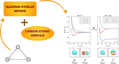
GRAPHICAL ABSTRACT

KEYWORDS:

• molecular structure
• strong magnetic fields
• excited states
• symmetry
• maximum overlap method

1. Introduction

The maximum overlap method (MOM) is an elegant and simple approach to calculate the electronic structure of excited states. The method was put forward by Gilbert, Besley and Gill in 2008 and has attracted more than 400 citations to date [1]. The MOM may be thought of as a practical implementation of the Δ-Self-Consistent Field (Δ-SCF) method [2–4]. It addresses a key issue in Δ-SCF calculations, namely the variational collapse to the lowest energy solution of a given spin symmetry. In the MOM approach, a simple orbital-overlap-based criterion is used to prevent the aforementioned variational collapse and excited states are targeted by selecting a non-Aufbau occupation from a set of ground-state reference orbitals. The MOM has been used in a wide range of applications such as X-ray spectroscopy [5–10], photoelectron spectroscopy [11,12], calculations of electronic excitation in crystalline solids [13], and vibrational analysis of excited states of molecules [14]. MOM solutions can also serve as reference wavefunctions for correlated methods [15–19].

The simplicity of the MOM is appealing, not only because it is easy to implement, but also because the MOM-SCF solutions are straightforward to interpret and use. A number of further developments of the MOM scheme have been put forward by many other authors including the initial MOM (IMOM) [20], projection-based MOM (PMOM) and projection-based initial MOM (PIMOM) [21]. It has also inspired work by other authors to provide alternative approaches to obtain Δ-SCF solutions for arbitrary excited states (see, for example, Refs. [22–24]). As a result, the original MOM paper has become one of the most highly cited and influential works of Nick Besley, to whose memory and scientific legacy this volume is dedicated.

In the present work, we propose harnessing the simple interpretive power of the MOM to understand the nature of molecular structure in the presence of strong magnetic fields. Recently, a wide range of electronic structure methods have been extended to treat molecules in external magnetic fields of arbitrary strength using London atomic orbitals (LAOs) [25–37]. The interplay between the kinetic and Coulombic terms of the electronic Hamiltonian with the extra terms arising due to the interaction with the external field leads to a complex variation of the energies of different electronic states with varying magnetic field. In particular, the crossing of states of different spin or involving orbitals of different angular momenta is a frequent occurrence, and so a simple approach for tracking different states, such as the MOM, is invaluable. Recent work has also led to the development of analytic nuclear gradients over LAOs [36] which enables the calculation of equilibrium molecular structures under these conditions. Coupling this development with the recent implementation of the MOM procedure using LAO-SCF methods [38] allows for the determination of the equilibrium molecular structures of excited states.

In the present work, we consider the simple molecules ${\text{H}}_3^{+}$ and ${\text{H}}_3$ in the presence of strong magnetic fields. The paper is organised as follows. In Section 2, we review key elements of the theoretical methods used; in particular, a brief overview of the MOM and its variants in strong magnetic fields is presented. In Section 3, we give the computational details of our calculations. In Section 4, we first discuss the potential energy surfaces of the lowest lying states of ${\text{H}}_3^{+}$ in a range of magnetic fields at equilateral geometries. Pronounced changes in the ordering of the different electronic states are observed, along with significant changes in the bonding in each state, as the magnetic field strength is increased. We then consider the fully optimised structures for each of these states and compare the lowest energy high-spin state of ${\text{H}}_3^{+}$ with the corresponding high-spin state of H₃. Finally, we interpret the structure of these states by considering the variation of their occupied molecular orbital (MO) energies as a function of bond angle in a magnetic field using constrained geometry optimisations. Concluding remarks and directions for future work are presented in Section 5.

2. Background and theory

2.1. Quantum chemistry in strong magnetic fields

The electronic Hamiltonian for an N-electron system in the presence of a uniform external magnetic field $\mathbf{B}$ is given by (1) $\begin{array}{rl}\hat{H}={\hat{H}}_0& +\sum _{i=1}^N\mathbf{B}\cdot {\hat{\mathbf{s}}}_i+\frac{1}{2}\sum _{i=1}^N\mathbf{B}\cdot {\hat{\mathbf{l}}}_i\\ & +\frac{1}{8}\sum _{i=1}^N[B^2{r}_i^2-(\mathbf{B}\cdot {\mathbf{r}}_i{)}^2],\end{array}$(1) where ${\hat{H}}_0$ is the standard zero-field electronic Hamiltonian. The remaining terms arise due to the presence of the external magnetic field and consist of the linear Zeeman terms depending on the spin (${\hat{\mathbf{s}}}_i$) and orbital angular momentum (${\hat{\mathbf{l}}}_i=-i{\mathbf{r}}_i\times {\mathbf{\nabla }}_i$) operators and a diamagnetic term that has a quadratic dependence on the external field strength. The linear Zeeman terms may either raise or lower the energy as a function of magnetic field and typically lift the degeneracy of orbitals; these terms often dominate at lower field strengths. However, as the field strength increases, the diamagnetic term, which always raises the energy, eventually dominates. The result is a complex variation of the electronic energy with the applied magnetic field, thus giving rise to potentially very rich chemistry. Given that zero-field degeneracies are lifted, with each component having a different response to the external field, state crossings and avoided crossings occur frequently as the field strength is increased. It is therefore highly desirable to have simple approaches to study many low-lying electronic configurations at modest computational cost so that the most relevant ones can be easily identified over a range of field strengths.

To perform quantum-chemical calculations, the Hamiltonian of Equation (1(1) $\begin{array}{rl}\hat{H}={\hat{H}}_0& +\sum _{i=1}^N\mathbf{B}\cdot {\hat{\mathbf{s}}}_i+\frac{1}{2}\sum _{i=1}^N\mathbf{B}\cdot {\hat{\mathbf{l}}}_i\\ & +\frac{1}{8}\sum _{i=1}^N[B^2{r}_i^2-(\mathbf{B}\cdot {\mathbf{r}}_i{)}^2],\end{array}$(1) ) may be employed directly, enabling studies for systems where the external magnetic field cannot be considered as a weak perturbation. The presence of the orbital angular momentum operator in the third term of Equation (1(1) $\begin{array}{rl}\hat{H}={\hat{H}}_0& +\sum _{i=1}^N\mathbf{B}\cdot {\hat{\mathbf{s}}}_i+\frac{1}{2}\sum _{i=1}^N\mathbf{B}\cdot {\hat{\mathbf{l}}}_i\\ & +\frac{1}{8}\sum _{i=1}^N[B^2{r}_i^2-(\mathbf{B}\cdot {\mathbf{r}}_i{)}^2],\end{array}$(1) ) means that the resulting wavefunctions may be complex and this must be accounted for in practical implementations. Moreover, for commonly used finite-basis-set approaches, the presence of the external field presents challenges with respect to the gauge-origin independence of observables and their convergence with respect to basis set size. To overcome these challenges, LAOs [39] can be used as basis functions with the form (2) ${\omega }_{\mathrm{a}}(\mathbf{r})={\varphi }_{\mathrm{a}}(\mathbf{r})\exp [-i\mathbf{A}({\mathbf{R}}_{\mathrm{a}})\cdot \mathbf{r}],$(2) where the complex phase factor is associated with a uniform magnetic field $\mathbf{B}$ via the vector potential $\mathbf{A}({\mathbf{R}}_{\mathrm{a}})=\frac{1}{2}\mathbf{B}\times ({\mathbf{R}}_{\mathrm{a}}-{\mathbf{R}}_{\mathrm{O}})$ for an LAO centred at ${\mathbf{R}}_{\mathrm{a}}$ relative to the gauge-origin ${\mathbf{R}}_{\mathrm{O}}$. This phase factor multiplies a standard Gaussian basis function ${\varphi }_{\mathrm{a}}(\mathbf{r})$. The use of LAOs ensures that calculated observables are gauge-origin independent and converge smoothly towards the basis set limit for arbitrary field strengths and orientations.

The introduction of LAOs for wavefunction-based approaches requires the evaluation of molecular integrals over these basis functions using complex algebra and implementations that do not assume real wavefunctions [33]. Several programs now exist that are capable of determining the required integrals over LAOs including London [40], BAGEL [41], ChronusQ [42], TURBOMOLE [43], CFOUR [44], QCUMBRE [45], and our in-house program QUEST [46]. Acceleration techniques such as the resolution of the identity (RI) [31,36,47] and Cholesky decomposition [48] are available. Analytic gradients are also available both with and without RI acceleration [26,36]. With the availability of the underlying integrals, a wide variety of electronic structure methods are now implemented for use in the strong-field regime using LAOs. These include Hartree–Fock (HF) theory [25], configuration interaction theory [28], complete active space self-consistent field (CAS-SCF) theory [31], coupled-cluster (CC) theory [32,35], (direct) random phase approximation and GW theories [49], as well as CAS-SCF with second-order perturbation theory [31]. For all of these approaches, the underlying electronic structure implementations follow through in a manner similar to their standard counterparts. However, significant implementation work is required to ensure compatibility with complex algebra and to ensure all assumptions associated with real wavefunctions are eliminated.

Density-functional theory (DFT) can also be extended to account for the presence of an external magnetic field. However, the universal density functional $F[\rho ,{\mathbf{j}}_{\mathrm{p}}]$ is then a functional of both the charge density ρ and the paramagnetic component of the induced current density ${\mathbf{j}}_{\mathrm{p}}$. It has recently been shown that the Vignale–Rasolt formulation [50,51] of current-DFT (CDFT) can be treated in a manner analogous to Lieb's formulation [52] of conventional DFT [27,53], placing it on a similarly rigorous mathematical foundation. A Kohn–Sham (KS) CDFT scheme can be set up in a non-perturbative manner using LAOs to describe the MOs — we refer the reader to Refs. [29,30,51] for details of the resulting KS equations. It therefore becomes necessary to approximate the exchange–correlation component $E_{\mathrm{xc}}[\rho ,{\mathbf{j}}_{\mathrm{p}}]$ in an appropriate manner. The accuracy of practical calculations using vorticity-based corrections to local density approximation (LDA) and generalised gradient approximation (GGA) levels has been shown to be poor [29,54,55]. However, introducing current dependence via the kinetic energy density at the meta-GGA level has been shown to yield good quality results in comparison with higher-level correlated approaches [30]. In the present work, we use the regularised form of the strongly constrained and appropriately normed (SCAN) semilocal density functional of Sun et al. [56], denoted r²SCAN, as proposed by Furness et al. [57]. The r²SCAN functional is based on the dimensionless kinetic energy density, (3) $\overline{\alpha }(\mathbf{r})=\frac{\tilde{\tau }(\mathbf{r})-{\tau }_{\mathrm{W}}(\mathbf{r})}{{\tau }_{\mathrm{unif}}(\mathbf{r})+\eta {\tau }_{\mathrm{W}}(\mathbf{r})},$(3) where ${\tau }_W(\mathbf{r})=|\mathrm{\nabla }\rho (\mathbf{r}){|}^2/8\rho (\mathbf{r})$ is the von Weizsäcker kinetic energy density, ${\tau }_{\mathrm{unif}}(\mathbf{r})=3(3{\pi }^2{)}^{2/3}{\rho }^{5/3}(\mathbf{r})/10$ is the kinetic energy density of a uniform electron gas, and (4) $\begin{array}{rl}\tilde{\tau }(\mathbf{r})& =\frac{1}{2}\sum _i^{\mathrm{occ}}[\mathrm{\nabla }{\phi }_i(\mathbf{r}){]}^{\ast }\cdot [\mathrm{\nabla }{\phi }_i(\mathbf{r})]-\frac{|{\mathbf{j}}_{\mathrm{p}}(\mathbf{r}){|}^2}{2\rho (\mathbf{r})}\\ & =\tau (\mathbf{r})-\frac{|{\mathbf{j}}_{\mathrm{p}}(\mathbf{r}){|}^2}{2\rho (\mathbf{r})},\end{array}$(4) is the everywhere positive kinetic energy density, which is modified here for use in a magnetic field in the manner discussed in Refs. [30,58–60] to ensure that the exchange–correlation energy remains properly gauge independent in the presence of a magnetic field, and where ${\phi }_i(\mathbf{r})$ are the KS orbitals. A simple regularisation using the parameter $\eta ={10}^{-3}$ was defined in Ref. [57] and helps to ensure that r²SCAN avoids the numerical instabilities suffered by the original SCAN functional [57,61]. Recently, global hybrid exchange–correlation functionals based on the r²SCAN have been developed [62]. They are constructed as (5) $E_{\mathrm{xc}}^{{\mathrm{r}}^2\mathrm{SCANx}}=(1-a)E_{\mathrm{x}}^{{\mathrm{r}}^2\mathrm{SCAN}}+a{E}_{\mathrm{x}}^{\mathrm{HF}}+E_{\mathrm{c}}^{{\mathrm{r}}^2\mathrm{SCAN}},$(5) with a denoting the amount of the HF exchange. Three variants of this functional with increasing amounts of the HF exchange have been developed: r²SCANh, r²SCAN0, and r²SCAN50 with $10\mathrm{\%}$, $25\mathrm{\%}$, and $50\mathrm{\%}$ of the HF exchange, respectively. It has been shown in Ref. [62] that a moderate amount of the HF exchange leads to a modest improvement of molecular properties over a wide range of benchmark data sets. In this work, we consider the use of the r²SCAN0 functional in strong magnetic fields.

2.2. The maximum overlap method

The MOM has been implemented in the QUEST program [38,46]. The implementation includes the original MOM approach of Gilbert, Besley and Gill [1] as well as the IMOM variant of Barca et al. [20] and the projection-based PMOM / PIMOM approaches of Corzo et al. [21]. Each MOM approach proceeds by tracking the SCF solution and choosing orbital occupations according to an overlap criterion rather than the more typical Aufbau-based one, driving the SCF solver towards a solution approximating a desired excited state.

The target orbitals, against which the SCF orbitals at each iteration are compared, and the metric used to determine the occupations distinguish the different variants of the MOM. For all MOM approaches, an initial set of MOs are generated for the ground state of the system of interest, and from these orbitals, excitations are then targeted by adjusting the occupations to replace one (or more) occupied orbitals by virtual orbitals in a manner consistent with the symmetry of the electronic excited state to be calculated. Typically, the orbitals used are those of the neutral ground state of the molecule, although in some cases it can be advantageous to also consider target orbitals from the ground state of the corresponding cationic system [1].

Once the initial orbital set has been selected, the ordinary MOM approach uses an overlap metric to select occupied SCF orbitals at a given iteration such that they are the ‘closest’ to, i.e. have the maximal overlap with, the target orbitals from the previous iteration. As a result, if one starts with orbitals occupied according to the excited state of interest, this method can be used to drive the SCF solver towards a solution closest to the desired excited state. In the IMOM approach of Barca and Gill [20], it was recognised that an alternative procedure is to occupy at each SCF cycle the orbitals most similar to target orbitals from the initial SCF guess which remain fixed throughout the SCF procedure. This alternative approach has been found to be beneficial in difficult cases such as doubly excited states.

In the MOM and IMOM approaches, the overlap metric used has been defined in a number of ways in the literature [1,15,20,63] — for an overview, see, for example, Ref. [21]. In the present work, we use the definition of Ref. [20]: (6) $s_p={\left\{\sum _i{[\sum _{\mu \nu }(C_{\mu i}^{\mathrm{target}}{)}^{\ast }{S}_{\mu \nu }{C}_{\nu p}]}^2\right\}}^{1/2},$(6) where the non-Aufbau occupations are selected in descending order of $\{s_p\}$. Here, $C_{\mu i}^{\mathrm{target}}$ are the target MO coefficients for the occupied orbitals, $S_{\mu \nu }$ is the overlap matrix in the atomic orbital (AO) basis, and $C_{\nu p}$ are the MO coefficients of the current SCF cycle.

More recently, the projection-based MOM approach was proposed by Corzo et al. [21], in which the overlap metric is calculated as (7) $s_p=\sum _q\sum _i\sum _{\mu \nu }\sum _{\lambda \sigma }{C}_{\mu p}^{\ast }{S}_{\mu \lambda }{C}_{\lambda i}^{\mathrm{target}}(C_{\sigma i}^{\mathrm{target}}{)}^{\ast }{S}_{\sigma \nu }{C}_{\nu q}.$(7) This projection is designed to select the set of eigenvectors of the current Fock matrix that gives rise to a determinant with the largest projection onto the determinant constructed from the target orbitals. This projection-based metric can be used with either target orbitals defined as those from the previous SCF iteration or the initial guess, denoted as PMOM or PIMOM, respectively. The implementation in the QUEST program has been extended to include these variants.

Despite many successes, the MOM does have some limitations. A well documented case is the description of open-shell singlet solutions, which cannot typically be well described by single-determinant methods. In these cases, the MOM typically leads to spin-contaminated solutions whose spin expectation values $⟨{\hat{S}}^2⟩$ are close to 1. This problem can be resolved to some extent by performing an approximate spin purification [64] for excitations of closed-shell molecules within the $M_S=0$ manifold. The simplest such approach is to calculate the energy of the corresponding triplet state in the $M_S=\pm 1$ manifold ($E_{\mathrm{T}}$), which is well represented by a single determinant, and then calculate the energy of the true singlet state according to (8) $E_{\mathrm{S}}=2E_{\mathrm{sc}}-E_{\mathrm{T}},$(8) where $E_{\mathrm{sc}}$ is the energy of the spin-contaminated solution. For a more detailed discussion, see, for example, Ref. [65]. A secondary point is that the MOM may be coupled with a variety of SCF algorithms, and in challenging cases, the solutions obtained may differ depending on the choice of SCF algorithm employed. In the present work, we utilise the MOM with the C1-DIIS approach [66,67] for convergence acceleration.

2.3. Symmetry analysis

In the presence of a magnetic field, the unitary symmetry point group of the molecule may be restricted to one of its subgroups since only symmetry operations that leave the combined molecule and field unchanged remain. In fact, the unitary symmetry group $\mathcal{H}$ of the system in a uniform magnetic field is given by the intersection $\mathcal{H}=\mathcal{G}\cap {\mathcal{C}}_{\mathrm{\infty }h},$where $\mathcal{G}$ is the zero-field unitary symmetry point group of the molecule and ${\mathcal{C}}_{\mathrm{\infty }h}$ is the well-known unitary symmetry group of the uniform magnetic field in the absence of any other external potentials [68,69]. In general, only proper or improper rotation axes parallel to the field, mirror planes perpendicular to the field, and the centre of inversion, if present, will remain. As such, the reduction $\mathcal{G}\supset \mathcal{H}$ depends on the orientation of the molecular frame relative to the direction of the applied magnetic field. Furthermore, it can be shown that all possible unitary symmetry groups in the presence of a magnetic field are Abelian [68,69].

In order to use the MOM procedure effectively, it is highly desirable to have knowledge of the unitary symmetry group $\mathcal{H}$ of the system so that the irreducible representations of $\mathcal{H}$ can be used to classify the symmetries of the SCF state and MOs. The latter are of course essential when deciding which MOs should be occupied for a particular target state using the MOM.

Thus far, only unitary symmetry has been discussed. In principle, when a magnetic field is present, certain antiunitary transformations involving the action of time reversal may also be symmetry transformations of the combined molecule and field [70–72]. In such a case, the full symmetry group of the system becomes a magnetic group [73], which is no longer unitary and for which corepresentations must be considered instead of representations [73–75]. However, antiunitary symmetry will not need to be taken into account in the present work because it turns out that unitary symmetry is more than sufficient to classify the SCF state and MOs for the purpose of utilising the MOM procedure for the systems examined in the discussions below. All of the unitary symmetry groups considered in this work are therefore subgroups of $\mathsf{O}(3)$.

To extract symmetry properties of SCF states and MOs automatically, a flexible symmetry analysis package QSym² has been developed and integrated into the QUEST program [46]. Details of the implementation and algorithms will be reported elsewhere; here we only indicate briefly some of its key capabilities that are relevant for the present work. In particular, QSym² is able to determine the unitary symmetry group $\mathcal{H}$ of any molecule in the absence or presence of magnetic and/or electric fields with arbitrary user-defined orientations without the need to impose a standard orientation. Then, the conjugacy classes are deduced and the character table is determined symbolically and automatically using the Burnside–Dixon algorithm [76,77]. This allows the conjugacy classes and irreducible representations of $\mathcal{H}$ to refer faithfully to the symmetry transformations of the system in the original user-defined orientation while also eliminating the need to store fixed character tables predefined in certain standard orientations.

Together with the generated character table, the general representation-theoretic approach described in Ref. [78] enables the Mulliken symmetry labels of SCF states and MOs to be determined directly in $\mathcal{H}$ without recourse to its Abelian subgroups. This approach ensures that degeneracy and symmetry breaking are correctly detected, and that any complex representations of $\mathcal{H}$, which occur frequently when $\mathcal{H}$ is an Abelian group in the presence of a magnetic field, are properly handled.

The classification of SCF states and MOs based on symmetry helps to ensure that the MOM solutions deliver the desired states, and that the correct states and MOs are followed as the molecular geometry and the applied magnetic field are varied. In the present work, we exploit this analysis to construct state and orbital correlation diagrams for systems in magnetic fields.

3. Computational details

The methods and analysis tools described in Section 2 have been implemented in our in-house QUEST program [46]. For all calculations, the 6-311(2+,2+)G(dp) basis set, which is augmented with additional diffuse functions as described in Refs. [1,79], was used. Geometry optimisations were carried out using the analytic-gradient implementation described in Ref. [36] with a quasi-Newton optimisation approach using the BFGS Hessian update scheme. All excited-state calculations use the IMOM approach of Ref. [20]. The MOM approach [1] was found to give similar results in the vast majority of cases, though some variational collapses were observed for larger magnetic field strengths. Preliminary investigations suggested that the PMOM and PIMOM approaches [21] give results identical to the MOM and IMOM for the simple ${\text{H}}_3^{+}$ and H₃ molecules in this study. Where potential energy curves are computed directly (see Sections 4.1 and 4.2), spatial symmetry breaking has been applied in the MOM calculations so that the curves approach the energies of the expected dissociation products.

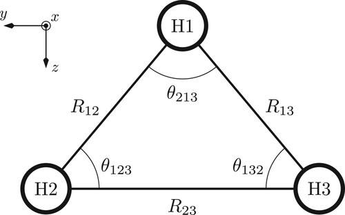
To analyse how the electronic structures of the high-spin states of ${\text{H}}_3^{+}$ and H₃ in a magnetic field determine the molecular structure, a series of constrained geometry optimisations were performed. Figure 1 shows a schematic of the molecular structure and defines the coordinates discussed in the present work. In particular, the direction of the applied magnetic field is defined relative to the Cartesian axes shown in Figure 1. Two constraints were applied in these calculations: first, the angle ${\theta }_{213}$ was constrained, allowing a scan to be carried out in which the molecules could be adjusted from a linear to bent structure allowing for the H−H distances to relax at each step; second, the molecular plane defined by the three hydrogen atoms was constrained to be perpendicular to the applied field vector. Both constraints were enforced by using an augmented Lagrangian approach requiring only the analytic nuclear gradient and first derivatives of constraint functions. Details of this approach will be reported in a forthcoming publication. All calculations were performed at the unrestricted Hartree–Fock (UHF) level. For comparison, geometry optimisations were also performed at the coupled cluster singles and doubles (CCSD) and r²SCAN0 levels of theory using numerical nuclear gradients.

Figure 1. Schematic of the atom numbering, bond labels and angles in ${\text{H}}_3^{+}$ and H₃.

4. Results and discussion

The H₂ molecule in strong magnetic fields was investigated by Kubo [80] and Lange et al. [28]. In the presence of a strong magnetic field on the order of $1B_0=235052\mathrm{T}$, the molecule preferentially orients perpendicular to the field direction and the $M_S=-1$ state (i.e. the $\beta (1)\beta (2)$ component of the zero-field ${}^3{\mathrm{\Sigma }}_u^{+}$ state) becomes the ground state. This observation is striking since the ${}^3{\mathrm{\Sigma }}_u^{+}$ state in the absence of a strong magnetic field is entirely repulsive, but becomes increasingly bound with stronger magnetic fields. This implies the possibility of a rather different chemistry in the presence of such extreme fields, which may be found on magnetic white dwarf stars.

In the present work, we consider ${\text{H}}_3^{+}$ and H₃ as prototypical examples of polyatomic systems. The ${\text{H}}_3^{+}$ cation is well studied as an important species in astrochemistry [81] which exhibits a ${\mathcal{D}}_{3h}$ equilateral triangular geometry in the ground state, whilst the H₃ radical has been much less studied and, as may be expected, is relatively unstable in the absence of a magnetic field. Several questions arise when considering molecular systems in the presence of a magnetic field. Which electronic configurations are favoured at each field strength? For each configuration, what is the preferred orientation relative to the applied field? What structure does a molecule adopt in the presence of an applied field? And finally, can the structure adopted be rationalised in a simple MO picture?

We use the prototypical ${\text{H}}_3^{+}$ and H₃ systems to examine some of these questions. The ground and lowest-lying excited states are determined in the absence of a field using the MOM protocol and then their behaviour is tracked to stronger magnetic fields. Optimised structures are determined for each state using the MOM within geometry optimisations and the features of the structures for the lowest-lying states are then rationalised using orbital correlation diagrams.

4.1. Potential energy surfaces for equilateral ${\text{H}}_3^{+}$

The ground ${}^1{A}_1^{\mathrm{\prime }}$ state of ${\text{H}}_3^{+}$ adopts an equilateral ${\mathcal{D}}_{3h}$ equilibrium geometry in the absence of a magnetic field. The ground state and the lowest excited states have been well studied computationally — see, for example, Ref. [82] for an early configuration-interaction investigation. We commence by considering this simple vertical excitation picture for the equilateral geometry in the presence of a range of magnetic fields.

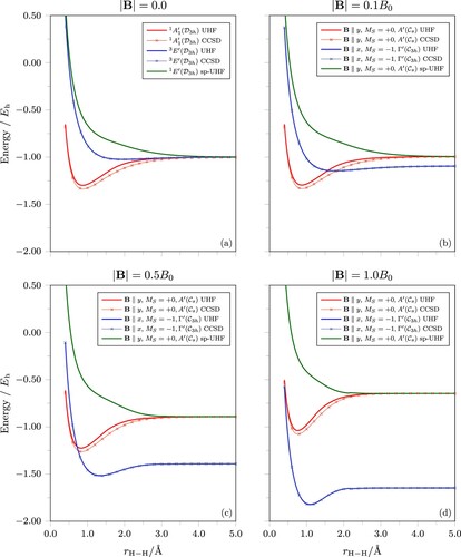
The potential energy curves for $|\mathbf{B}|=0.0,0.1,0.5$ and $1.0B_0$ are presented in Figure 2. The zero-field potential energy curves in Figure 2(a) agree well with those from higher level ab initio calculations [82], indicating that for the lowest states of this simple molecule, HF theory can provide a reasonable description. This is further confirmed by our own calculations at the CCSD level, as shown by the curves marked with crosses in Figure 2, and this agreement is preserved as the magnetic field strength increases. Similar potential energy curves can be obtained at the DFT level using the r²SCAN0 functional. However, the dissociation limits tend to be slightly too low in energy due to a residual self-interaction error and this affects each state to a different degree. As a result, we focus our discussion here on the HF and CCSD results and refer the reader to the supplementary material for a discussion of the r²SCAN0 results.

Figure 2. Potential energy curves for equilateral geometries of ${\text{H}}_3^{+}$ calculated using UHF, spin-purified UHF (sp-UHF), and CCSD. (a) The ${}^1{A}_1^{\mathrm{\prime }}$, ${}^1{E}^{\mathrm{\prime }}$ and ${}^3{E}^{\mathrm{\prime }}$ states in the absence of a magnetic field. (b) The corresponding $A^{\mathrm{\prime }}$, ${\mathrm{\Gamma }}^{\mathrm{\prime }}$ and $A^{\mathrm{\prime }}$ states in the presence of a magnetic field of magnitude $0.1B_0$. For states with $M_S=0$, the potential energy curves for the lowest energy orientation with the field vector parallel to the y-axis in Figure 1 is shown. For the state with $M_S=-1$, the lowest energy orientation with the field vector parallel to the x-axis (perpendicular to the molecular plane) is shown. (c) and (d) The corresponding $A^{\mathrm{\prime }}$, ${\mathrm{\Gamma }}^{\mathrm{\prime }}$ and $A^{\mathrm{\prime }}$ states in the presence of a magnetic field of magnitude 0.5 B₀ and 1.0 $B_0$, respectively.

As expected, the ${}^1{A}_1^{\mathrm{\prime }}$ ground state is bound, whilst the ${}^1{E}^{\mathrm{\prime }}$ and ${}^3{E}^{\mathrm{\prime }}$ states are dissociative in the absence of the magnetic field. Here, we have applied the approximate spin purification of Equation (8(8) $E_{\mathrm{S}}=2E_{\mathrm{sc}}-E_{\mathrm{T}},$(8) ) to the ${}^1{E}^{\mathrm{\prime }}$ state, taking care to remove the spin-Zeeman energy contribution from $E_{\mathrm{T}}$ when calculating the correction.

As a magnetic field is applied, there are several noteworthy changes to the electronic structure of ${\text{H}}_3^{+}$ for the states considered. Firstly, the states with $M_S=0$ preferentially orientate so that one of the H−H bonds is parallel to the field vector; this means that, in the coordinate system shown in Figure 1, $\mathbf{B}$ is parallel to the y-axis, denoted as $\mathbf{B}\parallel y$. In contrast, the state with $M_S=-1$ preferentially orientates with the field vector parallel to the x-axis — denoted as $\mathbf{B}\parallel x$ — and thus perpendicular to the molecular plane. In Figure 2(b–d), we therefore present each surface for the energetically preferred orientation.

In the presence of a magnetic field, the unitary symmetry group of equilateral ${\text{H}}_3^{+}$ is restricted to a subgroup of ${\mathcal{D}}_{3h}$ as discussed in Section 2, and the spatial symmetry labels of the states must be subduced accordingly. For the ground and excited singlet states which are labelled ${}^1{A}_1^{\mathrm{\prime }}({\mathcal{D}}_{3h})$ and ${}^1{E}^{\mathrm{\prime }}({\mathcal{D}}_{3h})$ in the absence of the field, the $\mathbf{B}\parallel y$ preferential orientation implies the restriction ${\mathcal{D}}_{3h}\supset {\mathcal{C}}_s$, for which the following subductions hold: $A_1^{\mathrm{\prime }}({\mathcal{D}}_{3h})\downarrow {\mathcal{C}}_s=A^{\mathrm{\prime }},E^{\mathrm{\prime }}({\mathcal{D}}_{3h})\downarrow {\mathcal{C}}_s=2A^{\mathrm{\prime }},$which means that, in $\mathbf{B}\parallel y$, the state ${}^1{A}_1^{\mathrm{\prime }}({\mathcal{D}}_{3h})$ becomes $A^{\mathrm{\prime }}({\mathcal{C}}_s)$, and the state ${}^1{E}^{\mathrm{\prime }}({\mathcal{D}}_{3h})$ is split into two non-degenerate states, each of which also has the label $A^{\mathrm{\prime }}({\mathcal{C}}_s)$. In what follows, only the energetically lower of the two $A^{\mathrm{\prime }}({\mathcal{C}}_s)$ states originating from ${}^1{E}^{\mathrm{\prime }}({\mathcal{D}}_{3h})$ shall be considered. In all cases, the spin projection quantum number $M_S=0$ remains a good descriptor with the spin projection axis taken to be along the direction of the magnetic field.

The splitting of the zero-field ${}^3{E}^{\mathrm{\prime }}({\mathcal{D}}_{3h})$ state is more subtle. In the absence of a field, this state has six microstates, all of which are degenerate, as a consequence of the spin triplet three-fold degeneracy and the spatial two-fold degeneracy. In the $\mathbf{B}\parallel x$ preferential orientation, the restriction ${\mathcal{D}}_{3h}\supset {\mathcal{C}}_{3h}$ holds, which admits the following subduction for the spatial part of the state: (9) $E^{\mathrm{\prime }}({\mathcal{D}}_{3h})\downarrow {\mathcal{C}}_{3h}={\mathrm{\Gamma }}^{\mathrm{\prime }}\oplus {\overline{\mathrm{\Gamma }}}^{\mathrm{\prime }},$(9) where ${\mathrm{\Gamma }}^{\mathrm{\prime }}$ and ${\overline{\mathrm{\Gamma }}}^{\mathrm{\prime }}$ are two one-dimensional complex-conjugate irreducible representations in ${\mathcal{C}}_{3h}$, and ${\mathrm{\Gamma }}^{\mathrm{\prime }}$ is chosen such that its character under the $C_3$ operation in the group (anticlockwise as viewed down the x-axis in Figure 1) is $\exp (2\pi i/3)$. Furthermore, the degeneracy between the three $M_S=0,\pm 1$ components of the spin triplet at zero field is lifted by the magnetic field. It turns out that the microstate with ${\mathrm{\Gamma }}^{\mathrm{\prime }}({\mathcal{C}}_{3h})$ spatial symmetry and $M_S=-1$ spin projection is the lowest amongst the six, which shall therefore be the only microstate originating from the zero-field ${}^3{E}^{\mathrm{\prime }}({\mathcal{D}}_{3h})$ state that will be considered for the rest of this discussion.

As the field is applied, the energies of the $A^{\mathrm{\prime }}({\mathcal{C}}_s)$ states rise diamagnetically. This can be seen easily by examining the red and green curves in Figure 2(b–d) at $5.0\text{Å}$ where their common dissociation limit of H($1s^{\alpha })$ + H($1s^{\beta })$ + H⁺ is approached: the energy of this dissociation limit rises purely due to the diamagnetic confinement of the electron on the hydrogen atoms, described by the last term of Equation (1(1) $\begin{array}{rl}\hat{H}={\hat{H}}_0& +\sum _{i=1}^N\mathbf{B}\cdot {\hat{\mathbf{s}}}_i+\frac{1}{2}\sum _{i=1}^N\mathbf{B}\cdot {\hat{\mathbf{l}}}_i\\ & +\frac{1}{8}\sum _{i=1}^N[B^2{r}_i^2-(\mathbf{B}\cdot {\mathbf{r}}_i{)}^2],\end{array}$(1) ). It is also clear that as $|\mathbf{B}|$ increases, the lower $A^{\mathrm{\prime }}({\mathcal{C}}_s)$ state, which corresponds to the ${}^1{A}_1^{\mathrm{\prime }}({\mathcal{D}}_{3h})$ state at zero field, remains bound, whilst the excited state, which corresponds to the ${}^1{E}^{\mathrm{\prime }}({\mathcal{D}}_{3h})$ state at zero field, remains unbound. The bound state in this equilateral geometry displays a minimum at shorter internuclear separations as $|\mathbf{B}|$ increases and both states also become degenerate and approach the dissociation limit at shorter internuclear distances as $|\mathbf{B}|$ increases. This is consistent with the analysis for the $M_S=0$ state of H₂ in Ref. [28] and illustrates the general features of binding in such states: diamagnetic confinement dominates, thus resulting in smaller atoms that can approach each other more closely but does not change fundamentally their bonding. In fact, the lowest $A^{\mathrm{\prime }}({\mathcal{C}}_s)$ state remains bound due to the double occupation of a bonding orbital, whilst the excited $A^{\mathrm{\prime }}({\mathcal{C}}_s)$ state remains unbound due to equal occupation of bonding and anti-bonding orbitals with electrons of opposite spin.

More striking is the behaviour of the ${\mathrm{\Gamma }}^{\mathrm{\prime }}({\mathcal{C}}_{3h})$ state as the magnetic field strength increases. The energy of this state is lowered paramagnetically by the spin-Zeeman contribution [the second term in Equation (1(1) $\begin{array}{rl}\hat{H}={\hat{H}}_0& +\sum _{i=1}^N\mathbf{B}\cdot {\hat{\mathbf{s}}}_i+\frac{1}{2}\sum _{i=1}^N\mathbf{B}\cdot {\hat{\mathbf{l}}}_i\\ & +\frac{1}{8}\sum _{i=1}^N[B^2{r}_i^2-(\mathbf{B}\cdot {\mathbf{r}}_i{)}^2],\end{array}$(1) )], resulting in a significant reordering of the states in Figure 2(b–d), with the ${\mathrm{\Gamma }}^{\mathrm{\prime }}({\mathcal{C}}_{3h})$ state becoming the lowest at all internuclear separations considered in a perpendicular field when $|\mathbf{B}|=1.0B_0$. Furthermore, the nature of the bonding in this state changes, from repulsive in the absence of a magnetic field to bound in the presence of a strong magnetic field with the dissociation energy increasing and the equilibrium internuclear separation decreasing as $|\mathbf{B}|$ increases. As a result, the bound $\beta (1)\beta (2)$ configuration of ${\text{H}}_3^{+}$ becomes increasingly more stable as the magnetic field increases compared to the H($1s^{\beta }$) + H($1s^{\beta }$) + H⁺ dissociation limit. This is consistent with the behaviour of the ${}^3{\mathrm{\Sigma }}_u^{+}$ state of H₂ as described in Ref. [28].

Throughout this analysis, we have assumed that the structure remains equilateral to give the simplified potential energy curves in Figure 2(a–d). This simple analysis reveals how the external magnetic field favours states with unpaired electrons that have β spin, and that different states may have different preferential orientations relative to the direction of the applied magnetic field. For the ${\mathrm{\Gamma }}^{\mathrm{\prime }}({\mathcal{C}}_{3h})$ state, the occurrence of perpendicular paramagnetic bonding is observed, as may be expected from Ref. [28]. Of course, for a polyatomic system, the molecular structure may distort away from the equilateral geometry — an aspect we shall consider in more detail in Section 4.3.

4.2. Potential energy surfaces for equilateral H₃

Given that the presence of a strong magnetic field favours systems with unpaired β-spin electrons, a natural point of comparison is the corresponding $M_S=-3/2$ state of H₃. In the absence of a magnetic field, this radical is very weakly bound in an equilateral geometry. However, in the presence of a strong magnetic field, the $M_S=-3/2$ state becomes the lowest in energy, with an equilateral geometry that preferentially orients perpendicular to the applied field. It is therefore interesting to compare this state of H₃ with those of ${\text{H}}_3^{+}$ considered in Section 4.1.

Potential energy curves for the equilateral geometry of H₃ in the $M_S=-3/2$ state are presented in Figure 3. In this configuration, the electrons are placed in the lowest three β MOs. Figure 3(a) shows clearly the paramagnetic decrease in the energy of the state with increasing $|\mathbf{B}|$, as would be expected from the presence of an additional electron with β spin which gives a larger spin-Zeeman contribution. However, for $|\mathbf{B}|<1.0B_0$, it is evident from the relatively flat potential energy curves that little or no binding occurs. Again, the HF and CCSD results agree remarkably well for this simple system in its high-spin configuration for all of the magnetic field strengths considered, indicating the modest role of correlation.

Figure 3. Potential energy curves of the lowest $M_S=-3/2$ state for equilateral geometries of H₃ at various magnetic field strengths. In all finite-field cases, the field vector is parallel to the x-axis and perpendicular to the molecular plane. At zero field, the system has ${\mathcal{D}}_{3h}$ unitary symmetry in which the state is given the symmetry label ${}^4{A}_2^{\mathrm{\prime }}$. At finite fields, the system is reduced to ${\mathcal{C}}_{3h}$ unitary symmetry and the state becomes $A^{\mathrm{\prime }}$ with spin-projection degeneracies lifted. (a) The UHF and CCSD energy curves. (b) The corresponding UHF and CCSD interaction energy curves given by $E(r_{\mathrm{H}-\mathrm{H}})-E(5.0\text{Å})$ plotted on a smaller vertical scale to show the variation of the minimum structures of the UHF and CCSD energy curves in (a) with respect to magnetic field strengths more clearly.

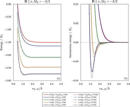
To investigate the nature of the interactions, further field strengths up to $|\mathbf{B}|=1.5B_0$ were considered. For $|\mathbf{B}|\ge 1.0B_0$, as seen in Figure 3(a), minima in the potential energy curves start to become perceptible. In Figure 3(b), the interaction energy relative to the H($1s^{\beta }$) + H($1s^{\beta }$) + H($1s^{\beta }$) dissociation limit is plotted for each field strength. It is clear that the field strength required to induce significant bonding in H₃ is much higher than that for ${\text{H}}_3^{+}$. A more detailed analysis of the bonding in each case is given in Section 4.4.

4.3. Optimised molecular structure for ${\text{H}}_3^{+}$ and H₃

For the bound states, geometry optimisations were performed to determine whether their structures would distort from the equilateral geometries considered in Sections 4.1 and 4.2. The geometrical parameters for the lowest energy orientations are summarised in Table 1 at the HF and CCSD levels, and in the supplementary information at the DFT level with the r²SCAN0 functional.

Table 1. Optimised molecular structures for the ${\text{H}}_3^{+}$ and H₃ molecules in particular electronic states as a magnetic field is applied either along the x ($B_x$) or y ($B_y$) directions as shown in Figure 1.

State	$M_S$	$\mathbf{B}/B_0$	Group	Symmetry	Energy / $E_{\mathrm{h}}$	${\theta }_{213}$ / ${}^{\circ }$	${\theta }_{132}$ / ${}^{\circ }$	$R_{12}$ / Å	$R_{23}$ / Å	Shape
${\text{H}}_3^{+}$
${}^1{A}_1^{\mathrm{\prime }}$	0	0	${\mathcal{D}}_{3h}$	$A_1^{\mathrm{\prime }}$	$-1.2985300$ $(-1.3372397)$	60.00	60.00	0.869 (0.878)	0.869 (0.878)	Equilateral
	0	$B_y=0.1$	${\mathcal{C}}_s$	$A^{\mathrm{\prime }}$	$-1.2953725$ $(-1.3340867)$	60.08 (60.09)	59.96 (59.96)	0.867 (0.875)	0.868 (0.877)	Isosceles
	0	$B_y=0.3$	${\mathcal{C}}_s$	$A^{\mathrm{\prime }}$	$-1.2707995$ $(-1.3095510)$	60.67 (60.74)	59.67 (59.63)	0.850 (0.858)	0.858 (0.868)	Isosceles
	0	$B_y=0.5$	${\mathcal{C}}_s$	$A^{\mathrm{\prime }}$	$-1.2246226$ $(-1.2634092)$	61.65 (61.83)	59.18 (59.08)	0.822 (0.830)	0.842 (0.852)	Isosceles
	0	$B_y=0.7$	${\mathcal{C}}_s$	$A^{\mathrm{\prime }}$	$-1.1607536$ $(-1.1995441)$	62.81 (63.13)	58.59 (58.44)	0.790 (0.798)	0.824 (0.835)	Isosceles
	0	$B_y=1.0$	${\mathcal{C}}_s$	$A^{\mathrm{\prime }}$	$-1.0391816$ $(-1.0779118)$	64.64 (65.17)	57.78 (57.42)	0.744 (0.751)	0.796 (0.809)	Isosceles
${}^3{E}^{\mathrm{\prime }}$	$-1$	0	${}^{†}$	–	–	–	–	–	–	–
	$-1$	$B_x=0.1$	${\mathcal{C}}_{3h}$	${\mathrm{\Gamma }}^{\mathrm{\prime }}$	$-1.1453838$ $(-1.1473844)$	60.00	60.00	1.762 (1.739)	1.762 (1.739)	Equilateral
	$-1$	$B_x=0.3$	${\mathcal{C}}_{3h}$	${\mathrm{\Gamma }}^{\mathrm{\prime }}$	$-1.3513473$ $(-1.3546006)$	60.00	60.00	1.516 (1.505)	1.516 (1.505)	Equilateral
	$-1$	$B_x=0.5$	${\mathcal{C}}_{3h}$	${\mathrm{\Gamma }}^{\mathrm{\prime }}$	$-1.5155514$ $(-1.5195295)$	60.00	60.00	1.349 (1.342)	1.349 (1.342)	Equilateral
	$-1$	$B_x=0.7$	${\mathcal{C}}_{3h}$	${\mathrm{\Gamma }}^{\mathrm{\prime }}$	$-1.6517855$ $(-1.6561028)$	60.00	60.00	1.226 (1.222)	1.226 (1.222)	Equilateral
	$-1$	$B_x=1.0$	${\mathcal{C}}_{3h}$	${\mathrm{\Gamma }}^{\mathrm{\prime }}$	$-1.8209581$ $(-1.8254658)$	60.00	60.00	1.093 (1.091)	1.093 (1.091)	Equilateral
${\text{H}}_3$
${}^4{A}_2^{\mathrm{\prime }}$	$-3/2$	0	${}^{†}$	–	–	–	–	–	–	–
	$-3/2$	$B_x=0.5$	${\mathcal{C}}_{3h}$	$A^{\mathrm{\prime }}$	$-2.0882040$ $(-2.0887421)$	60.00	60.00	2.203 (2.144)	2.203 (2.144)	Equilateral
	$-3/2$	$B_x=0.7$	${\mathcal{C}}_{3h}$	$A^{\mathrm{\prime }}$	$-2.2609694$ $(-2.2625532)$	60.00	60.00	1.794 (1.744)	1.794 (1.744)	Equilateral
	$-3/2$	$B_x=1.0$	${\mathcal{C}}_{3h}$	$A^{\mathrm{\prime }}$	$-2.4821822$ $(-2.4857342)$	60.00	60.00	1.445 (1.414)	1.445 (1.414)	Equilateral
	$-3/2$	$B_x=1.1$	${\mathcal{C}}_{3h}$	$A^{\mathrm{\prime }}$	$-2.5472857$ $(-2.5513931)$	60.00	60.00	1.369 (1.342)	1.369 (1.342)	Equilateral
	$-3/2$	$B_x=1.3$	${\mathcal{C}}_{3h}$	$A^{\mathrm{\prime }}$	$-2.6652456$ $(-2.6701932)$	60.00	60.00	1.258 (1.238)	1.258 (1.238)	Equilateral
	$-3/2$	$B_x=1.5$	${\mathcal{C}}_{3h}$	$A^{\mathrm{\prime }}$	$-2.7679688$ $(-2.7735027)$	60.00	60.00	1.179 (1.163)	1.179 (1.163)	Equilateral

${}^{†}$Dissociative.

Notes: Each state is labelled by the spin multiplicity and spatial symmetry that it would adopt in a ${\mathcal{D}}_{3h}$ molecular structure at zero field. Values are computed at the UHF and CCSD levels. CCSD values are shown in parentheses where different.

For the lowest $A^{\mathrm{\prime }}({\mathcal{C}}_s)$ state with $M_S=0$ which originates from the ${}^1{A}_1^{\mathrm{\prime }}({\mathcal{D}}_{3h})$ state at the equilateral configuration in zero field, ${\text{H}}_3^{+}$ is raised in energy as the magnetic field strength increases, as expected from Section 4.1. However, the structure smoothly distorts from the equilateral ${\mathcal{D}}_{3h}$ geometry obtained in the absence of a magnetic field to an isosceles structure with ${\mathcal{C}}_s$ symmetry. The equilibrium apex angle ${\theta }_{213}$ opens from ${60.00}^{\circ }$ to ${64.64}^{\circ }$ (${65.17}^{\circ }$) at the HF (CCSD) level as the field strength increases and the longest edge, H2−H3, aligns parallel to the applied field vector. The equilibrium H−H internuclear distances shorten significantly with changes on the order of $0.1\text{Å}$, with a slightly more pronounced shortening for $R_{12}$ and $R_{13}$ compared with $R_{23}$. This distortion allows the system to reduce its extent perpendicular to the field axis as the impact of the diamagnetic confinement [final term in Equation (1(1) $\begin{array}{rl}\hat{H}={\hat{H}}_0& +\sum _{i=1}^N\mathbf{B}\cdot {\hat{\mathbf{s}}}_i+\frac{1}{2}\sum _{i=1}^N\mathbf{B}\cdot {\hat{\mathbf{l}}}_i\\ & +\frac{1}{8}\sum _{i=1}^N[B^2{r}_i^2-(\mathbf{B}\cdot {\mathbf{r}}_i{)}^2],\end{array}$(1) )] becomes more important with increasing magnetic field.

For the ${\mathrm{\Gamma }}^{\mathrm{\prime }}({\mathcal{C}}_{3h})$ state with $M_S=-1$ of ${\text{H}}_3^{+}$ in a magnetic field, which corresponds to the ${}^3{E}_1^{\mathrm{\prime }}({\mathcal{D}}_{3h})$ state at the equilateral configuration in the absence of the field, the structure remains equilateral with the lowest energy orientation being that in which the molecular plane is perpendicular to the field direction. Initially, for $|\mathbf{B}|=0.5B_0$, a weakly bound minimum develops on this state as shown in Figure 2. However, as the field strength increases, the structure becomes increasingly bound and this is reflected in the significant shortening of equilibrium internuclear distances from $1.762\text{Å}$ at $|\mathbf{B}|=0.1B_0$ to $1.093\text{Å}$ at $|\mathbf{B}|=1.0B_0$.

For H₃ in its lowest $A^{\mathrm{\prime }}({\mathcal{C}}_{3h})$ state with $M_S=-3/2$, which corresponds to the ${}^4{A}_2^{\mathrm{\prime }}({\mathcal{D}}_{3h})$ state in the absence of a magnetic field, a similar trend is observed. The system remains equilateral and preferentially orients such that the molecular plane is perpendicular to the applied field. However, since H₃ is considerably less stable than ${\text{H}}_3^{+}$, the optimal structure calculated at $|\mathbf{B}|=0.5B_0$ has considerably larger internuclear H−H distances at $2.203\text{Å}$, than those for ${\text{H}}_3^{+}$ at $1.349\text{Å}$ in the same field strength at the HF level. As a result, significantly stronger fields are required to stabilise the structure, which is reflected in the shortening of the equilibrium internuclear H−H distances from $2.203\text{Å}$ to $1.179\text{Å}$ over the field range $|\mathbf{B}|=0.5-1.5B_0$. Overall, the results for both the ${\text{H}}_3^{+}$ and H₃ molecules computed at the CCSD level show a similar trend to those computed at the HF level (see Table 1).

4.4. MO analysis of bonding in strong magnetic fields

The analysis in Sections 4.1–4.3 highlights features of molecular bonding in a strong magnetic field. In this Section, we explore the extent to which the MO picture intrinsic to Δ-SCF and MOM calculations can be used to rationalise the nature of the structures of ${\text{H}}_3^{+}$ and H₃. In each case, we will focus on the states that become the ground state in strong magnetic fields.

A simple question is why the ${\mathrm{\Gamma }}^{\mathrm{\prime }}({\mathcal{C}}_{3h})$ state of ${\text{H}}_3^{+}$ and $A^{\mathrm{\prime }}({\mathcal{C}}_{3h})$ state of H₃ prefer to adopt an equilateral geometry in a strong field rather than an isosceles or linear structure, or, in particular, whether this preference can be rationalised in terms of maximising (minimising) bonding (anti-bonding) interactions in the MOs. To examine this question, we performed constrained geometry optimisations as described in Section 3 for a range of ${\theta }_{213}$ angles, varying from very acute through equilateral to linear.

4.4.1. $H_3^{+}$

In Figure 4(a), the variations of the occupied MO energies for the lowest $M_S=-1$ UHF solution of ${\text{H}}_3^{+}$ are shown for a range of ${\theta }_{213}$-constrained geometry-optimised structures with fields $\mathbf{B}\parallel x$ (perpendicular to the molecular plane), where ${20}^{\circ }\le {\theta }_{213}\le {180}^{\circ }$. The optimal equilateral structure has ${\mathcal{C}}_{3h}$ unitary symmetry in the perpendicular field and the occupied MOs adopt $A^{\mathrm{\prime }}$ and ${\mathrm{\Gamma }}^{\mathrm{\prime }}$ spatial symmetry. In each case, the orbital energies are presented relative to that of the highest occupied molecular orbital (HOMO) at the linear geometry for each field strength. The plots depict how each MO is stabilised or destabilised upon distorting the molecule away from the equilateral geometry and how this behaviour changes as $|\mathbf{B}|$ increases from $0.8B_0$ to $1.0B_0$. At all optimal isosceles geometries, the unitary group of the system in the field is reduced to ${\mathcal{C}}_s$ and the spatial symmetry labels of both MOs become $A^{\mathrm{\prime }}$. At the optimal linear geometry, the unitary symmetry group increases slightly to ${\mathcal{C}}_{2h}$ and the two MOs can be distinguished by spatial symmetry again, having $A_g$ and $B_u$ labels.

Figure 4. Variation of the lowest $M_S=-1$ UHF solution of ${\text{H}}_3^{+}$ in the presence of a uniform magnetic field $\mathbf{B}\parallel x$ across a range of ${\theta }_{213}$-constrained geometry-optimised structures. For each constrained value of ${\theta }_{213}$, all three H−H bond lengths in ${\text{H}}_3^{+}$ are allowed to relax to attain an optimal geometry. (a) Energies of the two occupied $m_s=-1/2$ MOs in ${\text{H}}_3^{+}$ along this path, plotted relative to the energy of the HOMO of the ${\theta }_{213}={180}^{\circ }$ geometry-optimised structure in each field strength. The forms of the two β MOs at ${60}^{\circ }$, ${120}^{\circ }$, and ${180}^{\circ }$ are also shown: the isosurface for MO ${\phi }_i(\mathbf{r})$ is plotted at $|{\phi }_i(\mathbf{r})|=0.08$, and the colour at each point $\mathbf{r}$ on the isosurface indicates the phase angle $\arg {\phi }_i(\mathbf{r})\in (-\pi ,\pi ]$ at that point according to the accompanied colour wheel. (b) Energy of the $M_S=-1$ UHF solution along this path, plotted relative to the value at the ${\theta }_{213}={180}^{\circ }$ geometry-optimised structure in each field strength.

To facilitate the understanding of how the MOs determine the bonding of the molecule, three-dimensional isosurface plots are used to illustrate their forms at the optimal geometries for ${\theta }_{213}={60}^{\circ }$, ${120}^{\circ }$, and ${180}^{\circ }$. Since the MOs are complex-valued in a magnetic field, the plotting method described in Ref. [83] is utilised together with VMD [84] to produce representations of the MOs that faithfully capture their complex phase structures which, as will become apparent shortly, play a crucial role in helping to rationalise their bonding nature.

In both Figure 4(a,b), a vertical dashed line is used to indicate the optimal equilateral geometry, which is also the globally optimal geometry. It is clear that there are two competing effects: at this geometry, the lower MO is least stable and would suggest a preference for an isosceles geometry, whereas the HOMO is most stabilised. As $|\mathbf{B}|$ increases, it can be observed that the HOMO is stabilised more significantly at the equilateral geometry than the lower MO is destabilised relative to the linear geometry. This is reflected in the fact that the total energy of the system minimises at the equilateral geometry as shown in Figure 4(b).

The nature of the MOs and the interaction with the magnetic field described by the Hamiltonian of Equation (1(1) $\begin{array}{rl}\hat{H}={\hat{H}}_0& +\sum _{i=1}^N\mathbf{B}\cdot {\hat{\mathbf{s}}}_i+\frac{1}{2}\sum _{i=1}^N\mathbf{B}\cdot {\hat{\mathbf{l}}}_i\\ & +\frac{1}{8}\sum _{i=1}^N[B^2{r}_i^2-(\mathbf{B}\cdot {\mathbf{r}}_i{)}^2],\end{array}$(1) ) rationalise both the observed stabilisation and de-stabilistion of each MO. The isosurface plots for the lower MO in Figure 4(a) reveal that this MO is mostly real-valued everywhere, and that the interaction between each pair of adjacent hydrogens is primarily in-phase and bonding. This MO is therefore unambiguously a bonding MO, which is consistent with the fact that its energy is significantly lower than that of the HOMO. However, to rationalise the observation that this MO is most unstable at the equilateral geometry, the confinement effects that lead to contraction of the orbital (and associated charge density) towards the nuclei must be considered.

The consequence of these effects is that, when the structure distorts away from the equilateral form, the more favourable electron-nuclear interaction energy arising from this contraction partially offsets the unfavourable repulsive interactions. For ${\theta }_{213}>{60}^{\circ }$, the structures are isosceles with the apex at H1 and $R_{12}$ and $R_{13}$ shorten as ${\theta }_{213}$ increases, enabling closer approaches of the smaller atoms in a magnetic field and stronger bonding interaction, thereby reducing the orbital energy. For ${\theta }_{213}$ decreasing from ${60}^{\circ }$ to ca. ${48}^{\circ }$, the structures remain isosceles with the apex at H1 and with the $R_{12}$ and $R_{13}$ distances increasing, consistent with maximising the bonding interaction between one pair of hydrogen atoms (i.e. H2−H3), whilst minimising the overall repulsion. At very acute angles ${\theta }_{213}<{48}^{\circ }$, repulsive interactions dominate and the structures distort further to become isosceles with the apex at H2 where the $R_{13}$ distance becomes longer as the angle becomes more acute. However, $R_{12}$ and $R_{23}$ decrease, and as a result, the orbital energy continues to fall due to favourable bonding interactions between H1−H2 and H2−H3. The change-over between the isosceles structures with the apex at H1 and those with apex at H2 occurs at ${\theta }_{213}\approx {48}^{\circ }$, which corresponds to the inflexion points on the energy curves for the lower MO in Figure 4(a).

On the other hand, the HOMO is more difficult to interpret owing to the generally complex-valued form of its isosurface plots as seen in Figure 4(a). To obtain a better appreciation for the bonding nature of this MO, one can consider an isoelectronic, but manifestly simpler, system: that of the lowest $M_S=-1$ state in H₂ which has term symbol ${}^3{\mathrm{\Sigma }}_u^{+}$ in the absence of magnetic fields. In Figure 5, the occupied MOs of the relevant states in ${\text{H}}_3^{+}$ and H₂ are compared at the respective geometries of the two structures optimised in a perpendicular magnetic field with strength $1.0B_0$. With the geometry kept fixed, each state is also smoothly followed with the aid of the MOM as the magnetic field is slowly switched off so that the unfamiliar finite-field complex-valued MOs can be correlated with the more familiar zero-field orbital pictures.

Figure 5. Isosurfaces of occupied MOs in the lowest $M_S=-1$ UHF solutions in ${\text{H}}_3^{+}$ and H₂ in the presence of a perpendicular magnetic field. For each molecule, the optimal geometry at $|{\mathbf{B}}_{\perp }|=1.0B_0$ is used to calculate the UHF solution, which is then tracked smoothly to $\mathbf{B}=\mathbf{0}$ with the help of the MOM as the field is switched off while keeping the geometry fixed. This is to generate the corresponding MOs at zero field for investigation purposes. The isosurface for MO ${\phi }_i(\mathbf{r})$ is plotted at $|{\phi }_i(\mathbf{r})|=0.08$, and the colour at each point $\mathbf{r}$ on the isosurface indicates the phase angle $\arg {\phi }_i(\mathbf{r})\in (-\pi ,\pi ]$ at that point according to the colour wheel shown in Figure 4.

${}^{†,‡}$ These MOs turn out to be slightly symmetry-broken at zero field, both of which having actual symmetry $A_1^{\mathrm{\prime }}\oplus E^{\mathrm{\prime }}$. This symmetry breaking, however, is not discernible from the isosurface plots and thus does not affect the qualitative argument given in the main text. Furthermore, as the perpendicular field is introduced, the MOs become symmetry-conserved.

It was shown by Lange et al. in Ref. [28] that the $1{\sigma }^{\ast }$ anti-bonding MO in H₂, which is shown as the ${\mathrm{\Sigma }}_u^{+}({\mathcal{D}}_{\mathrm{\infty }h})$ MO at zero field in Figure 5, is stabilised by a perpendicular magnetic field, and that this stabilisation is more effective for shorter internuclear separations. An examination of the ${\mathrm{\Sigma }}_u^{+}({\mathcal{D}}_{\mathrm{\infty }h})\to B_u({\mathcal{C}}_{2h})$ MO of H₂ in Figure 5 sheds light on this observation: as the magnetic field is applied perpendicular relative to the molecule, the mirror plane perpendicular to the H−H bond, which enforces the nodal plane in the ${\mathrm{\Sigma }}_u^{+}({\mathcal{D}}_{\mathrm{\infty }h})$ MO at zero field, is annihilated. Consequently, this MO, which has $B_u({\mathcal{C}}_{2h})$ symmetry in finite perpendicular fields, is allowed to have non-vanishing electron densities in the internuclear region and thus becomes partially bonding — this can be seen most prominently at $|{\mathbf{B}}_{\perp }|=1.0B_0$. Furthermore, the lack of a nodal plane means that points symmetric about this would-be plane are now no longer completely out-of-phase (i.e. they can now have phase differences less than π, which can be verified by examining the colouring of the isosurfaces in Figure 5). This therefore helps reduce the anti-bonding character of this MO.

This understanding can be transferred almost wholly to the $M_S=-1$ state in ${\text{H}}_3^{+}$. Let us consider first the optimal equilateral geometry of this system at $|{\mathbf{B}}_{\perp }|=1.0B_0$ for which the form of the HOMO is shown in Figure 4(a) and also in Figure 5. A quick comparison to its zero-field counterpart, which has symmetry label $E^{\mathrm{\prime }}({\mathcal{D}}_{3h})$ in Figure 5, shows that the perpendicular magnetic field destroys the vertical nodal plane passing through one of the protons (H1 using the labelling scheme in Figure 1) and perpendicular to the bond between the other two (H2−H3). This enables electron density to build up in the internuclear region between H2 and H3 in the HOMO in the $M_S=-1$ state of ${\text{H}}_3^{+}$. However, this is where the similarity with the $M_S=-1$ state in H₂ ends: the possibility of a third proton, H1, to now support electron density implies that there can now be electron interactions including all three H−H pairs. Moreover, the fact that this MO has symmetry ${\mathrm{\Gamma }}^{\mathrm{\prime }}$ in ${\mathcal{C}}_{3h}$, and thus a character of $\exp (2\pi i/3)$ under $C_3$, means that $C_3$-equivalent points in this MO are out-of-phase by only $2\pi /3$. Consequently, each H−H pair admits some weak bonding interaction, thereby reducing the overall anti-bonding character of this MO.

In light of the above description, it is now possible to return to Figure 4(a) to rationalise the shape of the energy curve for the HOMO in ${\text{H}}_3^{+}$. As the molecule distorts away from the equilateral geometry, for ${\theta }_{213}>{60}^{\circ }$, $R_{23}$ increases, and as a result, some of the stabilisation from the weak bonding interaction between H2 and H3 is lost, thus raising the energy of the orbital. For ${\theta }_{213}<{60}^{\circ }$, nuclear repulsive effects dominate, causing the structure to adjust in the same way as described previously for the lower MO, leading to larger separations between the atoms on average, further reducing the weak bonding interaction and resulting in the orbital energy increasing. At ${\theta }_{213}={60}^{\circ }$, the average distance between the atoms is minimised. As explained by symmetry, all three atoms can participate equally to maximise the stabilisation of the HOMO, which is the dominant factor in determining the overall equilateral molecular structure.

The orbital correlation plots in Figure 4 are somewhat similar to the classic Walsh diagrams [85] where the behaviour of the HOMO energy as a function of a molecular internal coordinate is used to rationalise the structure adopted. Typically, in constructing a Walsh diagram, only the coordinate of interest is varied, with all others kept fixed. However, preliminary studies in this work revealed that it is actually necessary to allow the internuclear distances to relax in order to observe the (de-)stabilisation of the MOs shown in Figure 4(a). This emphasises the need to traverse the potential energy curve along the lowest energy pathway corresponding to the distortion of the molecule.

4.4.2. H₃

Given that the presence of a strong external magnetic field strongly stabilises states with unpaired β-electrons via the spin-Zeeman interaction, it is interesting to consider a similar orbital correlation plot for the lowest energy $M_S=-3/2$ UHF solution of H₃ with $\mathbf{B}\parallel x$ (perpendicular to the molecular plane) in the range $0.5B_0\le |\mathbf{B}|\le 1.5B_0$. The additional occupied MO is found to have ${\overline{\mathrm{\Gamma }}}^{\mathrm{\prime }}({\mathcal{C}}_{3h})$ symmetry at the equilateral geometry, that reduces to $A^{\mathrm{\prime }}({\mathcal{C}}_s)$ and $A_g({\mathcal{C}}_{2h})$ symmetry at isosceles and linear geometries, respectively. The orbital energies are plotted relative to the energy of this HOMO in the linear geometry. As noted in Section 4.2, much stronger fields are required to induce significant binding in H₃. This is reflected in the total energy shown in Figure 6(a), which shows a minimum at the equilateral structure relative to the linear structure at a field strength of $1.5B_0$. This minimum has a similar depth to that observed for ${\text{H}}_3^{+}$ at a weaker field strength of $1.0B_0$.

Figure 6. Variation of the lowest $M_S=-3/2$ UHF solution of H₃ in the presence of a uniform magnetic field $\mathbf{B}\parallel x$ across a range of ${\theta }_{213}$-constrained geometry-optimised structures. For each constrained value of ${\theta }_{213}$, all three H−H bond lengths in H₃ are allowed to relax to attain an optimal geometry. (a) Energy of the $M_S=-3/2$ UHF solution along this path, plotted relative to the value at the ${\theta }_{213}={180}^{\circ }$ geometry-optimised structure in each field strength. (b)–(e) Energies of the three occupied β MOs plotted relative to the energy of the HOMO of the ${\theta }_{213}={180}^{\circ }$ geometry-optimised structure in each field strength. The forms of the β MOs at ${60}^{\circ }$, ${120}^{\circ }$, and ${180}^{\circ }$ are also shown: the isosurface for MO ${\phi }_i(\mathbf{r})$ is plotted at $|{\phi }_i(\mathbf{r})|=0.08$, and the colour at each point $\mathbf{r}$ on the isosurface indicates the phase angle $\arg {\phi }_i(\mathbf{r})\in (-\pi ,\pi ]$ at that point according to the colour wheel shown in Figure 4.

The orbital correlation plots in Figure 6(b–e) show that the ${\theta }_{213}$-variations of the energies of the lowest two occupied MOs, which shall henceforth be referred to as $\mathrm{HOMO}-1$ and $\mathrm{HOMO}-2$, are similar to those of the corresponding occupied MOs in ${\text{H}}_3^{+}$. However, these two MOs are much closer in energy in H₃ than in ${\text{H}}_3^{+}$. As $|\mathbf{B}|$ increases, the $\mathrm{HOMO}-1$ is stabilised at the equilateral structure whilst the $\mathrm{HOMO}-2$ is destabilised. Since these MOs have different symmetries at the equilateral ${\mathcal{C}}_{3h}$ geometry, they do not interact via the Fock operator, and so their energy curves may, and indeed do, approach each other closely [Figure 6(b–c)] and eventually cross at $|\mathbf{B}|\approx 0.9B_0$, resulting in a switch-around in the ${\mathcal{C}}_{3h}$ symmetry labels for these two MOs [Figure 6(d–e)]. However, at isosceles ${\mathcal{C}}_s$ geometries, both MOs, together also with the HOMO, are subduced to the same $A^{\mathrm{\prime }}$ symmetry and can therefore all interact with one another via the Fock operator. Hence, their energy curves can no longer cross, and if one were to plot orbital energy curves as functions of $|\mathbf{B}|$ at any fixed ${\theta }_{213}$ in the vicinity of ${60}^{\circ }$, one would observe an avoided crossing between the $\mathrm{HOMO}-1$ and $\mathrm{HOMO}-2$ around $|\mathbf{B}|\approx 0.9B_0$.

In a similar fashion to the HOMO in the $M_S=-1$ state of ${\text{H}}_3^{+}$ discussed in Section 4.4.1, the $\mathrm{HOMO}-1$ in the $M_S=-3/2$ state of H₃ is progressively more stabilised at the equilateral geometry relative to the linear one as $|\mathbf{B}|$ increases. However, this is counterbalanced by both the HOMO and the $\mathrm{HOMO}-2$ now being destabilised at this geometry with increasing $|\mathbf{B}|$. In both cases, however, the destabilisation of these orbitals relative to the linear geometry is less significant than the stabilisation of the $\mathrm{HOMO}-1$. Therefore, and rather interestingly, for H₃, it is then the behaviour of the $\mathrm{HOMO}-1$ that determines the molecular structure. Isosurfaces for the three MOs at ${\theta }_{213}={60}^{\circ }$, ${120}^{\circ }$, and ${180}^{\circ }$ are also shown in Figure 6. Clearly, the behaviours of $\mathrm{HOMO}-1$ and $\mathrm{HOMO}-2$ can be rationalised in a similar manner to those of the occupied MOs in ${\text{H}}_3^{+}$. For the HOMO, the preferred orientation is linear, with bending of the molecule leading to an increase in orbital energy. This example therefore highlights that the structure adopted under a strong magnetic field reflects the response of all of the occupied MOs to the field and may not be determined simply by the HOMO.

4.5. Consistency with the Jahn–Teller theorem

Thus far, the forms and variations of the occupied MOs have been analysed in detail to rationalise the observed optimal geometries of ${\text{H}}_3^{+}$ and H₃ in a number of electronic states. However, it is important to examine if and how these results are consistent with the more general symmetry-based predictions from the Jahn–Teller (JT) theorem [86]. To this end, let us first revisit the zero-field ground ${}^1{A}_1^{\mathrm{\prime }}({\mathcal{D}}_{3h})$ state in equilateral ${\text{H}}_3^{+}$. This state has no spatial degeneracy and is the only state that arises from the underlying electronic configuration $(a_1^{\mathrm{\prime }}{)}^2$, so the JT theorem posits that this state has a minimum at a high-symmetry ${\mathcal{D}}_{3h}$ geometry as there is no need for any molecular distortion to lift any degeneracy. The geometry optimisation results in Table 1 indeed confirm this. As a magnetic field is introduced along the y-axis, the molecule then responds by distorting away from the equilateral geometry, but this distortion is not of JT-type and can only be accounted for by a consideration of how the occupied MOs interact with the applied field, as done in Section 4.3.

Next, let us revisit the zero-field excited state ${}^3{E}^{\mathrm{\prime }}({\mathcal{D}}_{3h})$ in equilateral ${\text{H}}_3^{+}$. This state now has a double spatial degeneracy, and the JT theorem indicates that this state cannot be a minimum in the potential energy surface at ${\mathcal{D}}_{3h}$ geometries. The fact that the geometry optimisation results in Table 1 reveal the dissociative nature of this state is entirely consistent with the prediction by the JT theorem. However, as a magnetic field is applied perpendicular to the molecule, the double spatial degeneracy is lifted, and there is now no longer any requirement by the JT theorem for the molecule to distort to remove any spatial degeneracy to stabilise itself. The optimal form for the molecule is therefore equilateral, as observed.

Finally, consider the zero-field excited state ${}^4{A}_2^{\mathrm{\prime }}({\mathcal{D}}_{3h})$ in equilateral H₃. The fact that this state is not stable at ${\mathcal{D}}_{3h}$ geometries in the absence of a field (Table 1) despite the non-spatial-degeneracy can be surprising at first, but as the underlying electronic configuration for this state is $(a_1^{\mathrm{\prime }}{)}^1(e^{\mathrm{\prime }}{)}^2$, two additional states, ${}^2{E}^{\mathrm{\prime }}({\mathcal{D}}_{3h})$ and ${}^2{A}_1^{\mathrm{\prime }}({\mathcal{D}}_{3h})$, arise owing to the $(e^{\mathrm{\prime }}{)}^2$ contribution. These two states can interact through a ‘hidden’ pseudo-JT effect (cf. Section 4 of Ref. [86]) to give rise to a minimum lower than the original ${}^4{A}_2^{\mathrm{\prime }}({\mathcal{D}}_{3h})$ state at a distorted geometry. Introducing a perpendicular magnetic field lifts the degeneracy of the underlying $e^{\mathrm{\prime }}$ MOs and removes the need for the pseudo-JT distortion, thus allowing the equilateral structure to become a minimum on the potential energy surface, as observed.

5. Conclusions

We have shown how the use of the MOM in a magnetic field not only gives access to excited states and their properties in a simple manner, but also facilitates the interpretation of molecular structure under strong field conditions using a simple MO picture. Indeed, under these conditions, the MOM approach may be more readily applicable than in the absence of a field in some regards. For example, the $M_S=0$ manifold maybe less relevant under such conditions since the spin-Zeeman interaction favours the unpairing of β-electrons, and so, complications with open-shell singlet states and associated spin purification schemes may be less frequent.

The nature of chemical bonding for ${\text{H}}_3^{+}$ and H₃ was examined under strong field conditions. In many regards, features of the perpendicular paramagnetic bonding mechanism for H₂ examined in Ref. [28] are also observed in ${\text{H}}_3^{+}$ and H₃, as may be expected. However, the additional nucleus provides additional structural degrees of freedom and these prototypical systems reveal how molecular structure may be distorted under strong field conditions. In particular, the lowest $M_S=0$ state of ${\text{H}}_3^{+}$ was observed to adopt an isosceles structure with its largest H−H separation aligned with the applied magnetic field. In contrast, the lowest energy $M_S=-1$ state of ${\text{H}}_3^{+}$ and the $M_S=-3/2$ state of H₃ were found to orient preferentially perpendicular to the applied field with equilateral geometries.

To investigate why these structures are preferred, we constructed orbital correlation diagrams similar to those put forward by Walsh [85], using the MOs determined by MOM calculations with constrained geometry optimisation. The changes in the orbital energies along the lowest energy pathway for bending the molecules revealed that the structure of the lowest $M_S=-1$ state of ${\text{H}}_3^{+}$ is determined by its HOMO, which is significantly stabilised at the equilateral geometry. Interestingly, for H₃, this MO, despite not being the HOMO, is still key to determining the molecular structure under high fields — its preference for an equilateral geometry outweighing the preference of the other occupied MOs for a linear or isosceles geometry. In spite of this, the lowest $M_S=-3/2$ state of H₃ was found to become significantly bound only at quite high fields of strength $1.5B_0$. This is in contrast to the lowest $M_S=-1$ state of ${\text{H}}_3^{+}$ which is significantly bound in fields on the order of $1.0B_0$.

Overall, the results suggest that ${\text{H}}_3^{+}$ in its lowest $M_S=-1$ should be considered as a possible candidate molecule for observation on stellar bodies such as magnetic white dwarf stars. We expect that the simple MOM-based approach presented in this work will also be useful in qualitatively interpreting the behaviour of more complex species under strong magnetic fields.

Acknowledgements

We are grateful for access to the University of Nottingham's Augusta HPC service.

Disclosure statement

No potential conflict of interest was reported by the authors.

Correction Statement

This article has been corrected with minor changes. These changes do not impact the academic content of the article.

Additional information

Funding

We acknowledge financial support from the European Research Councilunder the European Union’s H2020 research and innovation programme/ERC Consolidator Grant topDFT [grant number 772259], and also financial support from the Norwegian Research Council through the CoE Hylleraas Centre for Quantum Molecular Sciences [grant number 262695].

References

- A.T.B. Gilbert, N.A. Besley and P.M.W. Gill, J. Phys. Chem. A 112, 13164 (2008). doi:10.1021/jp801738f
- P.S. Bagus, Phys. Rev. 139, A619 (1965). doi:10.1103/PhysRev.139.A619
- H. Hsu, E.R. Davidson and R.M. Pitzer, J. Chem. Phys. 65, 609 (1976). doi:10.1063/1.433118
- T. Ziegler, A. Rauk and E.J. Baerends, Theor. Chim. Acta 43, 261 (1977). doi:10.1007/BF00551551
- J. Lee, D.W. Small and M. Head-Gordon, J. Chem. Phys. 151, 214103 (2019). doi:10.1063/1.5128795
- T. Northey, J. Norell, A.E.A. Fouda, N.A. Besley, M. Odelius and T.J. Penfold, Phys. Chem. Chem. Phys. 22, 2667 (2020). doi:10.1039/C9CP03019K
- A. Bhattacherjee, C.D. Pemmaraju, K. Schnorr, A.R. Attar and S.R. Leone, J. Am. Chem. Soc. 139, 16576 (2017). doi:10.1021/jacs.7b07532
- A. Foerster and N.A. Besley, Chem. Phys. Lett. 757, 137860 (2020). doi:10.1016/j.cplett.2020.137860
- Y. Zhang, S. Mukamel, M. Khalil and N. Govind, J. Chem. Theory Comput. 11, 5804 (2015). doi:10.1021/acs.jctc.5b00763
- A.A.E. Fouda and N.A. Besley, J. Comput. Chem. 41, 1081 (2020). doi:10.1002/jcc.v41.11
- J.L. Mason, H. Harb, A.A. Taka, C.D. Huizenga, H.H. Corzo, H.P. Hratchian and C.C. Jarrold, J. Phys. Chem. A 125, 9892 (2021). doi:10.1021/acs.jpca.1c07818
- J.L. Mason, H. Harb, A.A. Taka, A.J. McMahon, C.D. Huizenga, H. Corzo, H.P. Hratchian and C.C. Jarrold, J. Phys. Chem. A 125, 857 (2021). doi:10.1021/acs.jpca.0c11002
- L.E. Daga and L. Maschio, J. Chem. Theory Comput. 17, 6073 (2021). doi:10.1021/acs.jctc.1c00427
- A.A. Taka, H. Corzo, A. Pribram-Jones and H. Hratchian, ChemRxiv (2022), doi:10.26434/chemrxiv-2021-cch5r-v2
- G.M.J. Barca, A.T.B. Gilbert and P.M.W. Gill, J. Chem. Phys. 141, 111104 (2014). doi:10.1063/1.4896182
- K.J. Oosterbaan, A.F. White and M. Head-Gordon, J. Chem. Theory Comput. 15, 2966 (2019). doi:10.1021/acs.jctc.8b01259
- J. Nite and C.A. Jiménez-Hoyos, J. Chem. Theory Comput. 15, 5343 (2019). doi:10.1021/acs.jctc.9b00579
- K.J. Oosterbaan, A.F. White, D. Hait and M. Head-Gordon, Phys. Chem. Chem. Phys. 22, 8182 (2020). doi:10.1039/C9CP06592J
- L.N. Tran, J.A.R. Shea and E. Neuscamman, J. Chem. Theory Comput. 15, 4790 (2019). doi:10.1021/acs.jctc.9b00351
- G.M.J. Barca, A.T.B. Gilbert and P.M.W. Gill, J. Chem. Theory Comput. 14, 1501 (2018). doi:10.1021/acs.jctc.7b00994
- H.H. Corzo, A.A. Taka, A. Pribram-Jones and H.P. Hratchian, J. Comput. Chem. 43, 382 (2021). doi:10.1002/jcc.v43.6
- K. Carter-Fenk and J.M. Herbert, J. Chem. Theory Comput. 16, 5067 (2020). doi:10.1021/acs.jctc.0c00502
- G. Levi, A.V. Ivanov and H. Jónsson, Faraday Discuss 224, 448 (2020). doi:10.1039/D0FD00064G
- D. Hait and M. Head-Gordon, J. Chem. Theory Comput. 16, 1699 (2020). doi:10.1021/acs.jctc.9b01127
- E.I. Tellgren, A. Soncini and T. Helgaker, J. Chem. Phys. 129, 154114 (2008). doi:10.1063/1.2996525
- E.I. Tellgren, S.S. Reine and T. Helgaker, Phys. Chem. Chem. Phys. 14, 9492 (2012). doi:10.1039/c2cp40965h
- E.I. Tellgren, S. Kvaal, E. Sagvolden, U. Ekström, A.M. Teale and T. Helgaker, Phys. Rev. A 86, 062506 (2012). doi:10.1103/PhysRevA.86.062506
- K.K. Lange, E.I. Tellgren, M.R. Hoffmann and T. Helgaker, Science 337, 327 (2012). doi:10.1126/science.1219703
- E.I. Tellgren, A.M. Teale, J.W. Furness, K.K. Lange, U. Ekström and T. Helgaker, J. Chem. Phys. 140, 034101 (2014). doi:10.1063/1.4861427
- J.W. Furness, J. Verbeke, E.I. Tellgren, S. Stopkowicz, U. Ekström, T. Helgaker and A.M. Teale, J. Chem. Theory Comput. 11, 4169 (2015). doi:10.1021/acs.jctc.5b00535
- R.D. Reynolds and T. Shiozaki, Phys. Chem. Chem. Phys. 17, 14280 (2015). doi:10.1039/C4CP04027A
- S. Stopkowicz, J. Gauss, K.K. Lange, E.I. Tellgren and T. Helgaker, J. Chem. Phys. 143, 074110 (2015). doi:10.1063/1.4928056
- T.J.P. Irons, J. Zemen and A.M. Teale, J. Chem. Theory Comput. 13, 3636 (2017). doi:10.1021/acs.jctc.7b00540
- T.J.P. Irons, L. Spence, G. David, B.T. Speake, T. Helgaker and A.M. Teale, J. Phys. Chem. A 124, 1321 (2020). doi:10.1021/acs.jpca.9b10833
- F. Hampe and S. Stopkowicz, J. Chem. Phys. 146, 154105 (2017). doi:10.1063/1.4979624
- T.J.P. Irons, G. David and A.M. Teale, J. Chem. Theory Comput. 17, 2166 (2021). doi:10.1021/acs.jctc.0c01297
- M. Wibowo, T.J.P. Irons and A.M. Teale, J. Chem. Theory Comput. 17, 2137 (2021). doi:10.1021/acs.jctc.0c01269
- G. David, T.J.P. Irons, A.E.A. Fouda, J.W. Furness and A.M. Teale, J. Chem. Theory Comput. 17, 5492 (2021). doi:10.1021/acs.jctc.1c00236
- F. London, J. Phys. Radium 8, 397 (1937). doi:10.1051/jphysrad:01937008010039700
- LONDON, A Quantum Chemistry Program for Plane–Wave/GTO Hybrid Basis Sets and Finite Magnetic Field Calculations <londonprogram.org>.
- T. Shiozaki, WIREs Computational Molecular Science 8, e1331 (2017). doi:10.1002/wcms.1331.
- D.B. Williams-Young, A. Petrone, S. Sun, T.F. Stetina, P. Lestrange, C.E. Hoyer, D.R. Nascimento, L. Koulias, A. Wildman, J. Kasper, J.J. Goings, F. Ding, A.E. DePrince, E.F. Valeev and X. Li, WIREs Comput. Mol. Sci. 10, e1436 (2019). doi:10.1002/wcms.1436.
- S.G. Balasubramani, G.P. Chen, S. Coriani, M. Diedenhofen, M.S. Frank, Y.J. Franzke, F. Furche, R. Grotjahn, M.E. Harding, C. Hättig, A. Hellweg, B. Helmich-Paris, C. Holzer, U. Huniar, M. Kaupp, A.M. Khah, S.K. Khani, T. Müller, F. Mack, B.D. Nguyen, S.M. Parker, E. Perlt, D. Rappoport, K. Reiter, S. Roy, M. Rückert, G. Schmitz, M. Sierka, E. Tapavicza, D.P. Tew, C. van Wüllen, V.K. Voora, F. Weigend, A. Wodyński and J.M. Yu, J. Chem. Phys. 152, 184107 (2020). doi:10.1063/5.0004635
- J.F. Stanton, J. Gauss, L. Cheng, M.E. Harding, D.A. Matthews and P.G. Szalay, CFOUR, Coupled-Cluster Techniques for Computational Chemistry, a Quantum-Chemical Program Package with Contributions from A. Asthana, A.A. Auer, R.J. Bartlett, U. Benedikt, C. Berger, D.E. Bernholdt, S. Blaschke, Y.J. Bomble, S. Burger, O. Christiansen, D. Datta, F. Engel, R. Faber, J. Greiner, M. Heckert, O. Heun, M. Hilgenberg, C. Huber, T.-C. Jagau, D. Jonsson, J. Jusélius, T. Kirsch, M.-P. Kitsaras, K. Klein, G.M. Kopper, W.J. Lauderdale, F. Lipparini, J. Liu, T. Metzroth, L.A. Mück, D.P. O'Neill, T. Nottoli, J. Oswald, D.R. Price, E. Prochnow, C. Puzzarini, K. Ruud, F. Schiffmann, W. Schwalbach, C. Simmons, S. Stopkowicz, A. Tajti, J. Vázquez, F. Wang, J.D. Watts, C. Zhang, X. Zheng, and the Integral Packages MOLECULE (J. Almlöf and P.R. Taylor), PROPS (P.R. Taylor), ABACUS (T. Helgaker, H.J. Aa. Jensen, P. Jørgensen, and J. Olsen), and ECP routines by A.V. Mitin and C. van Wüllen. For the Current Version, see <https://www.cfour.de>.
- Quantum Chemical Utility Enabling Magnetic-Field Dependent Investigations Benefitting from Rigorous Electron-Correlation Treatment (2022). <https://www.qcumbre.org/>.
- QUEST, a Rapid Development Platform for QUantum Electronic Structure Techniques (2022). <https://quest.codes>.
- A. Pausch and W. Klopper, Mol. Phys. 118, e1736675 (2020). doi:10.1080/00268976.2020.1736675
- S. Blaschke and S. Stopkowicz, J. Chem. Phys. 156, 044115 (2022). doi:10.1063/5.0076588
- C. Holzer, A.M. Teale, F. Hampe, S. Stopkowicz, T. Helgaker and W. Klopper, J. Chem. Phys. 150, 214112 (2019). doi:10.1063/1.5093396
- G. Vignale and M. Rasolt, Phys. Rev. Lett. 59, 2360 (1987). doi:10.1103/PhysRevLett.59.2360
- G. Vignale and M. Rasolt, Phys. Rev. B 37, 10685 (1988). doi:10.1103/PhysRevB.37.10685
- E.H. Lieb, Int. J. Quantum Chem. 24, 243 (1983). doi:10.1002/(ISSN)1097-461X
- S. Kvaal, A. Laestadius, E. Tellgren and T. Helgaker, J. Phys. Chem. Lett. 12, 1421 (2021). doi:10.1021/acs.jpclett.0c03422
- A.M. Lee, N.C. Handy and S.M. Colwell, J. Chem. Phys. 103, 10095 (1995). doi:10.1063/1.469912
- W. Zhu and S.B. Trickey, J. Chem. Phys. 125, 094317 (2006). doi:10.1063/1.2222353
- J. Sun, A. Ruzsinszky and J.P. Perdew, Phys. Rev. Lett. 115, 036402 (2015). doi:10.1103/PhysRevLett.115.036402.
- J.W. Furness, A.D. Kaplan, J. Ning, J.P. Perdew and J. Sun, J. Phys. Chem. Lett. 11, 8208 (2020). doi:10.1021/acs.jpclett.0c02405
- J.F. Dobson, J. Chem. Phys. 98, 8870 (1993). doi:10.1063/1.464444
- A.D. Becke, Can. J. Chem. 74, 995 (1996). doi:10.1139/v96-110
- J.E. Bates and F. Furche, J. Chem. Phys. 137, 164105 (2012). doi:10.1063/1.4759080
- A.P. Bartók and J.R. Yates, J. Chem. Phys. 150, 161101 (2019). doi:10.1063/1.5094646
- M. Bursch, H. Neugebauer, S. Ehlert and S. Grimme, J. Chem. Phys. 156, 134105 (2022). doi:10.1063/5.0086040
- N.A. Besley, A.T.B. Gilbert and P.M.W Gill, J. Chem. Phys. 130, 124308 (2009). doi:10.1063/1.3092928
- K. Yamaguchi, F. Jensen, A. Dorigo and K. Houk, Chem. Phys. Lett. 149, 537 (1988). doi:10.1016/0009-2614(88)80378-6
- D. Hait and M. Head-Gordon, J. Phys. Chem. Lett. 12, 4517 (2021). doi:10.1021/acs.jpclett.1c00744
- P. Pulay, Chem. Phys. Lett. 73, 393 (1980). doi:10.1016/0009-2614(80)80396-4
- P. Pulay, J. Comput. Chem. 3, 556 (1982). doi:10.1002/(ISSN)1096-987X
- A.J. Ceulemans, Group Theory Applied to Chemistry (Springer, Dordrecht, 2013).
- A. Pausch, M. Gebele and W. Klopper, J. Chem. Phys. 155, 201101 (2021). doi:10.1063/5.0069859
- R.R. Birss, Symmetry and Magnetism (North-Holland Pub Co, Amsterdam, 1966).
- P. Lazzeretti, M. Malagoli and R. Zanasi, in Nuclear Magnetic Shieldings and Molecular Structure, edited by J.A. Tossell (Springer Science+Business Media, B.V., Maryland, 1993), p. 163.
- S. Pelloni and P. Lazzeretti, Int. J. Quantum Chem. 111, 356 (2011). doi:10.1002/qua.22658
- C.J. Bradley and B.L. Davies, Rev. Mod. Phys. 40, 359 (1968). doi:10.1103/RevModPhys.40.359
- E. Wigner, Group Theory and Its Application to the Quantum Mechanics of Atomic Spectra (Academic Press, London, 1959), p. 386.
- A.P. Cracknell, Prog. Theor. Phys. 35, 196 (1966). doi:10.1143/PTP.35.196
- J.D. Dixon, Numer. Math. 10, 446 (1967). doi:10.1007/BF02162877
- L.C. Grove, Groups and Characters (John Wiley & Sons Inc, New York, USA, 1997).
- B.C. Huynh and A.J.W. Thom, J. Chem. Theory Comput. 16, 904 (2020). doi:10.1021/acs.jctc.9b00900
- C.M. Hadad, J.B. Foresman and K.B. Wiberg, J. Phys. Chem. 97, 4293 (1993). doi:10.1021/j100119a010
- A. Kubo, J. Phys. Chem. A 111, 5572 (2007). doi:10.1021/jp070809z
- T. Oka, Philos. Trans. R. Soc. A 370, 4991 (2012). doi:10.1098/rsta.2012.0243.
- K. Kawaoka and R.F. Borkman, J. Chem. Phys. 54, 4234 (1971). doi:10.1063/1.1674665
- R. Al-Saadon, T. Shiozaki and G. Knizia, J. Phys. Chem. A 123 (14), 3223 (2019). doi:10.1021/acs.jpca.9b01134
- W. Humphrey, A. Dalke and K. Schulten, J. Mol. Graph. 14, 33 (1996). doi:10.1016/0263-7855(96)00018-5
- A.D. Walsh, J. Chem. Soc. 2260 (1953). doi:10.1039/jr9530002260
- I.B. Bersuker, in The Jahn–Teller Effect – Fundamentals and Implications for Physics and Chemistry, edited by Horst Köppel, David R. Yarkony and Heinz Barentzen (Springer, Heidelberg, 2009), pp. 3–23.