Dynamical and interference effects in X-ray emission spectroscopy of H-bonded water – origin of the split lone-pair peaks

Abstract

We examine the effects of core-hole-induced dynamics and vibrational interference on computed x-ray emission spectra of H-bonded water. Two model pentamers were investigated, tetrahedral and distorted, representing possible local environments in proposed low- and high-density water. Core-hole-induced dynamics were considered in the simulations, and the semi-classical Kramers-Heisenberg (SCKH) scheme to convolute theoretical spectra was applied. We determine the origin of the split two peaks in XES of liquid water to be a combination of the initial H-bonding and subsequent dynamics, where we find faster dynamics for tetrahedrally bonded. We further find that H-bond acceptors move towards the core-excited molecule while donors move away and we analyse the origin of this dynamics in terms of charge-redistributions during the dynamics.

We determine the origin of the split two peaks in X-ray emission spectra of liquid water to be a combination of the initial H-bonding and subsequent dynamics, where we find faster dynamics for tetrahedrally H-bonded water. We further find that H-bond acceptors move towards the core-excited molecule while donors move away and we analyse the origin of this dynamics in terms of charge-redistributions during the dynamics.

GRAPHICAL ABSTRACT

KEYWORDS:

• X-ray emission
• water
• XES

1. Introduction

Water is indispensable for living organisms and exhibits anomalies in a large number of its properties [1–4]. Among the most well-known are the solid being less dense than the liquid, the density maximum at 4°C, the minima in isothermal compressibility (κ_T) and heat capacity at constant pressure (C_P) at 46 and 35°C, respectively. These anomalies emerge naturally in two-state thermodynamical models of water that build on a balance between enthalpy and entropy in the free energy of the liquid as described by low- (LDL) and high-density liquid (HDL) [5–7] or locally favored structures versus density [8–10]. The proposed existence of two liquid states and a phase transition between them in the metastable part of the phase diagram was inspired by the existence of the first-order-like transition between the low- (LDA) and high-density amorphous (HDA) ices that exist at temperatures below the glass transition [11,12]. By heating samples of HDA it has been possible experimentally to follow the transition from HDL to LDL and thus confirm the existence of the two different liquids [13,14]. These experiments are very challenging since, in this ‘No man’'s land’ region, water crystallises too quickly for conventional measurement techniques.

In computer simulations, on the other hand, various water models have been used to investigate the liquid in search for the liquid–liquid critical point that would terminate the coexistence line in this metastable region, i.e. at temperatures below that of homogeneous ice nucleation, but above the glass transition temperature (see, e.g. summary in Ref. [4]). The coexistence of two minima in the free energy, characterised as HDL and LDL liquid based on the density and Q₆ parameter, was unequivocally demonstrated for ST2 water by Palmer et al. [15]; this concluded a long-standing debate among simulators on the possible existence of two forms of the liquid in the deeply supercooled and pressurised region of the phase diagram, a phase transition between them and the existence of a second critical point terminating their coexistence line [16–23].

At a critical point the correlation length becomes infinite and fluctuations between the two phases occur on all length scales leading to divergence in properties such as κ_T and C_P [24]. In the single-phase region beyond the critical point, lines of maxima in correlation length, κ_T and C_P emanate as extensions of the coexistence line. For supercooled water this so-called Widom line has recently been determined experimentally [25,26] and also in simulations of a large number of force-field models, but typically with a large offset in pressure. However, in recent simulations using the MB-pol model, a quantitative agreement with the experimental data for the maximum in κ_T was obtained [27] indicating that structural fluctuations are accurately reproduced. In a two-state picture of water, such structural fluctuations would persist also in ambient water, albeit in terms of more local fluctuations on some time-scale into LDL-like environments in the otherwise more HDL-like liquid [28,29]. Since ambient conditions lie beyond the proposed location of the critical point [13,25] terminating the experimentally observed liquid–liquid coexistence line [13,14,25], ambient water is a single phase of the liquid. However, as with any single-phase region beyond a critical point, there is a remaining imprint in terms of fluctuations that diminish in magnitude with distance from the critical point; this remaining imprint in terms of a balance between components favored by entropy or enthalpy has been shown to be essential in thermodynamical models to reproduce the anomalous properties of water [4,6–8,31]. Experimental support for this more bimodal local structural picture of ambient water is also provided by, e.g. Raman spectroscopy [32–34], decomposition of the temperature-dependent IR spectrum by Maréchal [35], small-angle x-ray scattering by Huang et al. [28], and soft x-ray vibrational spectroscopy by Harada and coworkers [36,37]. However, with x-ray absorption (XAS) and emission spectroscopy (XES) there is a discussion independent of this now experimentally, and also from thermodynamical considerations and simulations, established broader picture of the liquid water phase diagram, whether XAS and XES provide support for or contradict this picture of ambient water.

X-ray absorption and emission spectra of liquid water exhibit temperature-dependent features that have been interpreted in terms of contributions from molecules in two classes of local environments characterised in terms of HDL- and LDL-like [28–30,36–46]. However, this assignment is under debate and the validity of conclusions on water structure based on x-ray spectroscopy questioned [47–56]. Especially the interpretation of the double peaks observed in the range of 525–526 eV in x-ray emission spectroscopy (XES) of liquid water has been debated. Fuchs et al. [54,55] proposed that the double-peak structure can be reproduced by a continuous liquid model with the two peaks assigned to, respectively, dissociated and molecular species, but what determines the temperature-dependent branching ratio between the two is a challenge in a continuous model [57]. That XAS and XES support a continuum picture of water was also recently proposed by Niskanen et al. [56], but criticised in a comment [58]. Yamazoe et al. [59] investigated directly the influence of dissociated species and showed that dissociation affects the spectrum, but does not generate the split peaks. It is thus of importance to more deeply investigate the dynamics following core-ionisation, as is the object of the present study.

Very recently one of the authors and his coworkers [60] reported theoretical XES spectra of liquid water based on molecular dynamics simulations using the TIP4PEw force-field for geometry sampling and density functional theory (DFT) for the XES calculations. Core-hole-induced dynamics (CHID) was included as classical Born-Oppenheimer dynamics with quantum initial conditions from sampling six vibrational degrees of freedom (internal modes and librations). The XES spectra were constructed using the semi-classical Kramers-Heisenberg (SCKH) formalism developed by Ljungberg et al. [61–63]. In this work, not only the temperature, but also the isotope dependence reported by Tokushima et al. [46] were reproduced qualitatively, albeit with a too large split between the two peaks. The origin of the split was concluded to be a combination of dynamics and initial H-bonding.

The finding of two peaks in the lone-pair 1b₁ region was surprising since earlier work using the same approach, but sampling only the high-energy stretch modes resulted in a single 1b₁ peak and it had been argued that the lower-energy modes would not contribute significantly to the dynamics [44,46,57]. More recently, the present authors have computed XES spectra at the multiconfiguration SCF level including CHID, sampling the quantum probability distribution of all degrees of freedom of the targeted molecule and generated the spectrum using the same SCKH approach as above. However, only a single dominating 1b₁ peak was obtained, but with a low-intensity peak at ∼1.6 eV lower energy. Only by a Monte Carlo fit to the experimental XES spectrum of the computed spectra from a large number of situations could agreement with experiment be obtained, i.e. a different distribution of H-bond situations than obtained directly from the simulation was required [64]. Based on analysis of the structures that contributed to fit the experiment, a trend towards bimodality and more structured distributions than given by the force-field was concluded. However, the contrasting results of refs. [60] and [64] warrant further investigation, although the overall conclusion that the split is due to a combination of initial H-bonding and dynamics remains.

Zhovtobriukh et al. [43] performed TDDFT calculations of XES in collaboration with Nick Besley, focusing on the dependence of the 1b₁ position on the initial H-bonding geometry. They concluded that molecules with distorted and elongated H-bonds give the high-emission-energy peak while tetrahedrally H-bonded molecules with short and well-defined H-bonds contributed to the low-emission-energy peak. However, in that work it was not possible to include CHID. To elucidate the contribution of CHID and initial H-bonding situation to the XES spectrum of liquid water more clearly, we here follow earlier work by Nick Besley [65] and investigate a simpler model system. Water pentamer is a suitable and minimum size model of possible H-bonding situations in liquid water which will be the focus of the present work. We will here use two pentamers, a tetrahedral and a distorted, that can be considered as representing either LDL and HDL local environments or as end-points in a continuum distribution of structures.

2. Computational method

Two pentamer model structures are considered, i.e. a tetrahedrally coordinated water cluster as representative of the local coordination in the proposed low-density liquid (LDL) and a distorted water cluster, as proposed for the high-density liquid (HDL) [38]. The former is a double-donor/double-acceptor (D2A2) species with four surrounding water molecules positioned tetrahedrally with all O-O distances involving the central oxygen set to 2.8 Å, which corresponds to the first peak of the radial distribution function of liquid water [66]. The geometrical parameters related to hydrogen atoms of the surrounding oxygen atoms were taken from Ref. [67]. The disordered model cluster is a single-donor/single-acceptor (D1A1) with the O-O distance to the two H-bonded waters set to 2.95 Å, which is slightly longer than that for D2A2 to mimic the effect of a sixth water in the interstitial region (not explicitly included in the model). The O-O distance to the non-H-bonded waters was set to 3.6 Å to be well separated from the central water molecule giving a well-defined D1A1 species. The structure of the centre water molecule was optimised with the other four water molecules frozen.

XES is a photon-in/photon-out spectroscopy, which can be viewed as a one-step scattering process. The Kramers-Heisenberg formula for a non-resonant (i.e. independent of excitation energy) transition as function of the frequency of the emitted photon ω’ is given by [62], (1) $\begin{array}{r}\sigma ({\omega }^{\mathrm{\prime }})={\sum _f\left|\sum _n\frac{⟨f|D^{\mathrm{\prime }}|n⟩⟨n|D|i⟩}{{\omega }^{\mathrm{\prime }}-E_{nf}+i\mathrm{\Gamma }}\right|}^2,\end{array}$(1) where i, n, and f denote the initial, intermediate, and final states, E_nf is the energy difference between intermediate and final states, and Γ is the lifetime broadening. D’ and D are the dipole operators of the emission process and incoming radiation.

Especially for systems including light elements, such as hydrogen, the time scale of molecular vibrations is comparable to the lifetime of the core-hole, i.e. a few fs. Furthermore, removing one screening 1s electron in the oxygen in a water molecule effectively transforms it into H₂F⁺ which initiates proton transfer along any donated H-bonds the molecules is involved in. At normal H-bond distances in liquid water or ice there is no barrier to this transfer, which means that the zero-point energy stored in the internal OH-bond will be released. Thus, it is important to include dynamical effects in the computational scheme and in particular to account for the quantum probability distributions in both positions and momenta of the protons [57,62,63,68]; the latter becomes particularly significant for the OH-stretch modes, since their zero-point energy exceeds k_BT by close to an order of magnitude at ambient conditions. The former is instead of more importance for the softer modes that have small momenta, but a broad spatial distribution.

The time-evolution of the core-ionised system corresponds to wave packet motion on the multi-dimensional potential energy surface of the system, which for larger water cluster becomes unrealistic to precompute. Instead, we apply a semi-classical (SCKH) approximation[62] to Equation (1) which builds on averaging over classical core-hole-induced dynamics (CHID) trajectories with initial geometry and momentum sampling of the zero-point vibrational motion; in these calculations, the oxygen of the central water thus had an explicit core hole, i.e. one 1s electron removed.

The spectrum is built as (2) $\begin{array}{r}\sigma ({\omega }^{\mathrm{\prime }})=\sum _{\text{traj}}\sum _F{|D_F^{+}({\omega }^{\mathrm{\prime }})|}^2,\end{array}$(2) where the transition amplitude $D_F^{+}({\omega }^{\mathrm{\prime }})$ is given by (3) $\begin{array}{rl}{D}_F^{+}({\omega }^{\mathrm{\prime }})& ={\int }_0^{\mathrm{\infty }}dt{D}_{NI}^{+}(0)D_{FN}^{+}(t)\\ & \times e^{-{\int }_0^t(E_F(\tau )-E_N(\tau ))d\tau }{e}^{-\mathrm{\Gamma }t}{e}^{-i{\omega }^{\mathrm{\prime }}t}\end{array}$(3) The amplitude $D_F^{+}({\omega }^{\mathrm{\prime }})$ in Equation (3) is thus given as the Fourier transform of the autocorrelation between the amplitude to transition from the initial state to the intermediate electronic state at time zero and the amplitude to go to the final state at a later time t. This is damped by the exponential lifetime decay factor $e^{-\mathrm{\Gamma }t}$. The Fourier transform in Equation (3) converts the trajectories in the time domain, with step-wise computed spectrum contributions, into a continuous spectrum in the energy domain. This approach preserves the important interference effects between vibrational intermediate states in the wave packet evolution. The SCKH approach has been shown to accurately describe XES from liquid methanol [69] and ethanol [70], which represent H-bonded systems, but without the complication of uncertainties in the structures obtained from molecular dynamics simulations.

To determine proper initial conditions for the CHID, consistent with the quantum probability distributions, we have first optimised the structure of the central molecule in the fixed geometry of the other four and computed the harmonic frequencies and corresponding normal modes. The normal modes are normalised and orthogonal to each other and can thus be used to build a product vibrational wave function describing the zero-point distribution of the central molecule; the Fourier transform of this distribution gives the corresponding momentum distribution. All nine degrees of freedom of the central molecule were included, i.e. three vibrational, rotational and translational modes; since the molecule is in a bound state also the librational and translational modes were approximated as harmonic. The appropriate reduced mass of each mode was used and velocities distributed according to the relative masses of the three particles in the molecule.

The normalised normal modes describe the motion around the optimised minimum, but cannot be expected to be valid for large deviations. The total energy for each normal mode as function of distortion along the mode was thus computed in the ground state system to determine the maximum sampling range consistent with the available zero-point energy of that mode (Supplementary Material). This product distribution was then sampled (positions and momenta) to generate initial conditions for the subsequent dynamics, while requiring the probability of each set to exceed 0.2; an unbiased sampling of an 18-dimensional (9 positions and momenta) distribution would otherwise result predominantly in states with extremely low weight. The total number of sampled initial conditions was 60, which is sufficient to obtain converged calculated spectra.

After the initial conditions were determined, the CHID, with an explicit core-hole on the central water, was propagated for 20 fs in steps of 0.25 fs. We confirmed that 20 fs is sufficient to obtain converged spectra for time propagation because of the short core-hole lifetime of ∼4 fs at the O K-edge [71,72]. XES spectra were calculated at each time-step along the trajectories using the ground-state approximation, i.e. neglecting relaxation effects both in the core-ionised and valence-ionised states [73]. The CHID and spectrum calculations were performed using the deMon2k density functional programme [74]. The standard Perdew–Burke–Ernzerhof (PBE) gradient-corrected exchange–correlation functional [75] with [3s/1p] basis sets for hydrogen, [7s/6p/2d] IGLO-III basis sets [76] for the core-excited oxygen in the central water molecule, and [2s/2p] basis sets with relativistic effective core potentials for the remaining oxygens were used. The vibrational frequencies of the central molecule were obtained using the Gaussian16 code [77]. Life-time vibrational interference effects [68] in the final spectra were included using the SCKH approach [61–63].

The SCKH scheme requires access to the PES of the ground and intermediate state and all final states in order to construct the vibrational wave functions that give rise to the interference effects. The core-hole PES was obtained directly from the CHID while the ground state PES was obtained as a byproduct of the XES spectrum calculations, which were performed using the ground state orbitals [73]. The PES:s for the final states (valence-hole) were approximated as the ground state energy minus the orbital energy for each valence state. Note that this ensures that the large effect of core-hole relaxation is included in the transition energies that are determined as the difference between core-hole and valence-hole PES:s. Valence-hole relaxation is assumed constant which leads to a slight compression of the computed spectra.

Each trajectory, however, is obtained as a time-ordered sequence of energy-ordered transitions (final states) where the order of the actual states typically varies along the trajectory. Connecting transitions simply in their order of appearance at each time-step results in smooth PES:s, but with large jumps in cross-section as states actually cross or interact at different time-steps. Since the transformation from the time-domain to obtain the cross-section in terms of emission energy is through the Fourier transform in Equation (3), this leads to a broadening of transitions and smearing out of spectral features unless such final-state curve-crossings and interactions are taken into account. To correctly disentangle the potential energy curves and eliminate such discontinuities in the transition moments, a genetic algorithm developed by the authors [78] was applied. This algorithm is useful to improve the resolution of the XES spectra.

A simplified two-step model to include the CHID has been used by several authors in earlier work (see discussion in Ljungberg et al. [62]). Here the excitation and de-excitation processes are treated separately, essentially amounting to neglecting the initial excitation as well as interference effects. The spectra are calculated at the specific geometry at each time step with either a Lorentzian broadening as [62] (4) ${\sigma }_{\text{traj}}^{t_i}[{\omega }^{\mathrm{\prime }},R(t_i)]=\sum _F\frac{{|D_{\text{FN}}^{\mathrm{\prime }}[R(t_i)]|}^2}{{\{{\omega }^{\mathrm{\prime }}-E_{\text{NF}}[R(t_i)]\}}^2+{\mathrm{\Gamma }}^2}$(4) or Gaussian broadening (5) $\begin{array}{rl}{\sigma }_{\text{traj}}^{t_i}[{\omega }^{\mathrm{\prime }},R(t_i)]& =\sum _F|D_{\text{FN}}^{\mathrm{\prime }}[R(t_i)]{|}^2{e}^{-x^2/{\sigma }^2},\\ x& ={\omega }_{\text{FN}}-{\omega }^{\mathrm{\prime }},\end{array}$(5) where $\sigma =\mathrm{\Gamma }/\sqrt{\text{ln}2}$ gives the Gaussian broadening in terms of the life-time broadening $\mathrm{\Gamma }$. Here, $\mathrm{\Gamma }$ is the half-width-at-half maximum (HWHM) of the Lorentzian in Equations (1) and (4). Assuming that the core-level is broadened only by life-time broadening, the core-hole life-time τ is obtained as $\tau =\frac{\hslash }{2\mathrm{\Gamma }}$ with $2\mathrm{\Gamma }$ being the full-width-at-half-maximum (FWHM) and $\mathrm{\Gamma }$ estimating the uncertainty in energy. In both cases the total spectrum is summed over all trajectories with an exponential damping factor corresponding to the lifetime τ of the core hole, (6) ${\sigma }_{\text{total}}({\omega }^{\mathrm{\prime }})=\sum _{\text{traj}}\sum _i{\sigma }_{\text{traj}}^{t_i}[{\omega }^{\mathrm{\prime }},R(t_i)]e^{-t_i/\tau }$(6) Note that the exponential decay factor in Equation (6) is consistent with the definition in Equation (20) in ref. [62] by recognising $\mathrm{\Gamma }$ as the HWHM, rather than the FWHM.

3. Results and discussion

3.1. XES of pentamers with different H-bond configurations

Figure 1A shows calculated XES spectra of the two model pentamers using the SCKH formalism, including life-time vibrational interference effects through CHID using 60 initial conditions randomly sampled from the zero-point distribution; we emphasise that the dynamics discussed in the following always refers to that induced by the creation of the core-hole. Based on the molecular orbitals of the single molecule we assign the three regions in the spectrum in order of increasing emission energy as 1b₂, 3a₁, and 1b₁ using the molecular C_2v point group. We note a split of ∼0.5 eV between the peaks of 1b₁ character with the tetrahedral D2A2 pentamer giving rise to the peak at lower-emission energy. This split is rather small compared to the experimental range 0.7–0.9 eV [46] with 0.8 eV at room temperature [59]. Our model systems are two different pentamers, which are good for trends, but insufficient to describe the splitting in the liquid quantitatively.

Figure 1. (A) Computed SCKH spectra of D1A1 (black) and D2A2 (red) pentamers. The peaks are labelled with the corresponding molecular valence orbitals from which they derive. (B) The same as in (A) but without the dynamics, i.e. spectra computed for the initial geometry of each trajectory and then summed for each of the D1A1 and D2A2 models.

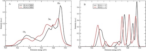
In Figure 1B we show, for the same two structures, the XES spectra at t = 0, i.e. summing over spectra computed only for the initial geometries and neglecting the CHID. Due to sampling around the initial geometry and perturbations from the surrounding water molecules, we observe a split and broadening in each region even at t = 0. We note that already in the initial geometry we find the D1A1 1b₁ peak at higher emission energy than for the D2A2 pentamer. The split is significantly smaller, 0.2 eV, compared to when CHID is included, showing that in this case a major contribution to the split comes from the dynamics where the D2A2 1b₁ shifts more towards lower energy than the D1A1 peak.

However, these two model structures are clearly insufficient to draw quantitative conclusions and for a definitive analysis we prefer a computed spectrum that reproduces experiment. For a proper analysis of the origin of the split we thus analyse further the computed spectrum from ref. [64], which was obtained by a Monte Carlo procedure to generate weights to apply to the summation of computed spectra to reproduce the experiment. The spectra were calculated using SCKH following the scheme presented here, but with CHID and spectra computed at the QM/MM level using multiconfigurational restricted active space SCF (RASSCF) wave functions rather than DFT as used in the present work. Some 3400 structures from simulations of the liquid were included, however, a fitting procedure (SpecSwap-RMC [79]) was still required to obtain agreement with experiment. This procedure yielded weights that can be applied to reweigh other properties to correspond to distributions that are consistent with the fitted experimental data. Below, we will apply the derived weights to decompose the full spectrum in terms of H-bonding situation as well as to derive the spectrum at t = 0 that with CHID evolves into the spectrum that reproduces the experiment.

In Figure 2A we show the fitted spectrum from ref. [64] together with its decomposition in terms of various H-bond donor species using the H-bond definition of Wernet et al. [38] with R_max= 3.3 Å; the corresponding decomposition in terms of acceptor species is given in the Supplementary Material. In Figure 2B we show in black the spectrum at t = 0 summed with the same weights that for the spectrum with CHID gives agreement with experiment; i.e. the spectrum in Figure 2B develops into the spectrum in Figure 2A with the CHID. Without CHID we observe a separation of the contributions of the differently H-bonded species such that D2 species are found at lower emission energy while D1 and D0 species contribute at higher energy. The decomposition in terms of H-bond donor contributions thus shows a split of 0.5 eV already without dynamics between single- and double-donor species. With the CHID this grows to the experimental ∼0.8 eV [46], where the peak at higher emission energy is given uniquely by D1 and D0 species while the other peak has contributions from both D2 and D1 species. The D0 species spectra do not exhibit any significant effects of CHID, apart from broadening of the peaks in the 3a₁ and 1b₂ regions. Thus, the observable split appears as function of the CHID, but is present already in the original structure and determined by the initial H-bonding environment. The CHID is important, but determined by the initial H-bonding situation. Similar to the present D2A2 pentamer, the effect of CHID in terms of peak position is thus larger for the D2 species as evidenced by the increased split compared to the smaller split without CHID. In ref. [60] stronger effects of CHID and weaker dependence on H-bond situation were found, which may have been due to sampling the normalised vibrational modes without restricting the sampling by the actually available zero-point energy.

Figure 2. (A) Decomposition of the fitted XES spectrum (black) from ref. [64] in terms of number of donated H-bonds. The decomposition into contributions from D0 (red), D1 (green) and D2 (blue) species is shown. (B) The corresponding spectrum contributions without CHID.

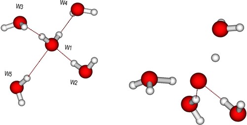
In the following we will focus on the data presented in Figure 1 and analyse the effect of the CHID by depicting the time-evolution of the OH bond lengths of the central water up to 20 fs in Figure 3A,B. The two hydrogens of the D2A2 species (Figure 3A) both undergo dynamics and stretch symmetrically as has been observed earlier [80]. There is a variation and spread depending on the initial conditions, but during the first 7 fs both hydrogens move away in a concerted motion along the H-bond direction, which persists also at longer times for the majority of the trajectories. After about 10 fs most trajectories exhibit the maximum elongation as the hydrogens reach the accepting oxygen and are reflected back as expected if the kinetic energy is not dissipated on the relevant time-scale. Clearly, however, in the majority of cases both internal O-H bonds will be significantly elongated when the core-hole decays, resulting in more atomic-like decay. In Figure 4 we show an example structure from a D2A2 trajectory where both protons have moved significantly towards the accepting waters; the snapshot corresponds to 8 fs, i.e. close to the maximum separation for one of the protons.

Figure 3. Time-evolution of internal OH-bond-lengths with CHID for (A) D2A2 and (B) D1A1 model pentamers.

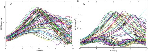
Figure 4. (Left) Initial pentamer structure defining H-bond donors (W2, W5) and acceptors (W3, W4) with respect to the central molecule. The D2A2 and D1A1 model pentamers differ in the W4, W5 bond lengths, which are elongated for the D1A1 species. (Right) Example snapshot after 8 fs of a D2A2 trajectory where both protons are significantly distanced from the oxygen.

For the D1A1 model we confirm the picture from earlier work [80] that, for non-resonant excitation, the H-bonded OH undergoes CHID while the non-H-bonded remains essentially unaffected. We note that the situation is the opposite for resonant excitation at the XAS pre-edge, i.e. into the 4a₁ antibonding state localised on the non-H-bonded OH [36,45,81,82], which causes this OH to dissociate while the H-bonded OH is basically unaffected. In the present case we again see a maximum elongation around 10 fs but the maximum deviation shows a much greater spread in time depending on the initial conditions compared to for the D2A2 species, indicating faster dynamics in the latter case. Only one of the 60 sampled trajectories can be said to have led to complete dissociation on the investigated time-scale; all other trajectories have the H-bonded hydrogen moving towards the accepting oxygen and then returning. In the case of D1A1 species at least one hydrogen remains closely associated with the central oxygen during the XES emission thus essentially making the emission occur from an OH radical species (the proton carries away the positive charge).

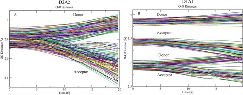
In Figure 5 we show the evolution of the O-O distances involving the central oxygen where Figure 4 gives the definition of donating and accepting molecules. For both D2A2 and D1A1 species, we observe as a general trend that the H-bond accepting molecules move closer to the central molecule while the molecules donating an H-bond move to longer distance.

Figure 5. Time evolution of O-O distances for the (A) D2A2 and (B) D1A1 model pentamers. Donor molecules (W2, W5) in Figure 4 move to larger distance while acceptors (W3, W4) are attracted to the central oxygen as the proton(s) move towards the acceptor. The difference in initial elongated donor and acceptor distance (3.4 vs 3.8 Å) for the D1A1 species is due to the optimisation, where the central molecule has been free to move towards the acceptor; the further spread around these distances is due to the sampling of the zero-point distribution (including translations) of the central molecule.

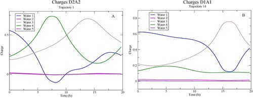
The time-evolution of the total Mulliken charge on each molecule along two example trajectories is shown in Figure 6. For this analysis, we kept the definition of the central molecule as including the oxygen and the two hydrogens, independent of where the two hydrogens were. The Mulliken analysis is sufficient in the present case since rather limited basis sets are used on the surrounding molecules, such that ambiguities in the charge assignments are minimised. The positive charge due to the creation of the core hole is initially mainly localised on the central water (W1), but some charge has already at the initial time step been transferred from the H-bond-accepting W3 and W4 water molecules to screen the core hole (see Figure 4 for definitions); the H-bond donating W2 and W5 molecules are unaffected in terms of charge transfer along the trajectories. As the proton moves towards the accepting oxygen, it picks up charge and becomes close to neutral and instead the positive charge gets transferred to the accepting water. For the D1A1 pentamer (Figure 6B) only one proton undergoes dynamics, while for the D2A2 pentamer (Figure 6A) both protons move along the H-bonds. In the particular trajectory in Figure 6A, this occurs sequentially with nearly full charge transfer at the turning points at the accepting waters.

Figure 6. Charge on individual waters as function of time along two example CHID trajectories. (A) D2A2 pentamer and (B) D1A1 pentamer.

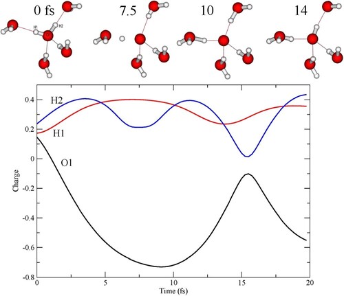
The charge evolution along the trajectory in Figure 6A is analysed further in Figure 7, where instead the individual charges on the atoms of the central molecule are given together with example structural snapshots. Initially, the positive charge is more or less evenly distributed on the molecule, but as the protons move towards the accepting waters they each carry a positive charge, which results in a negatively charged central atomic-like oxygen. The maximum negative charge occurs around 10 fs, where both protons are more closely associated with the accepting waters. After around 14 fs proton H2 has returned to the central oxygen and effectively neutralised the charge, while proton H1 is still associated with water W3. While this lasts, the central oxygen with the core-hole is effectively part of an OH radical, but we note that there is no sign of charge transfer to make an OH⁻ species. In earlier experimental work [54], resonant excitation of OH⁻ in solution has been used to suggest that the low-emission energy 1b₁ peak is due to dissociated molecules, while the peak at higher energy was proposed to be due to intact molecules. This has been criticised [55,57] and instead the peaks were assigned as originating from molecules in different H-bonding situations. Both interpretations have merit, although rather in terms of structures that are only transient on the time-scale of the core-hole lifetime. We do find that there is an initial difference in peak position due to the H-bonding situation, which increases with the CHID. The dynamics depend on the H-bonding situation, such that with one well-defined donated H-bond the emission occurs essentially from an OH radical associated with an extra proton, which is more or less delocalised as a wavepacket between the two oxygens [63]. With two well-defined donated H-bonds, on the other hand, both protons become delocalised and the emission becomes more atomic-like, as an O⁻ loosely associated with the two delocalised proton distributions.

Figure 7. Mulliken charge on each of the atoms in the central molecule as a function of time along the trajectory in Figure 6A.

Next, we discuss the initial distance dependence of XES of the tetrahedral D2A2 pentamer. Figure 8(a) shows XES as function of OO distances R(OO), with all OO distances being equal and varied from 2.6 to 3.0 Å. The shortest R(OO) is compressed compared to the 2.8 Å in the liquid while the longer R(OO) is expanded. We especially focus on the peak around 530 eV, assigned as 1b₁. At R(OO) = 3.0 Å, a sharp peak is obtained although split by 0.7 eV at t = 0. By decreasing R(OO), the splitting at t = 0 becomes larger and is 1.5 eV at R(OO) = 2.6 Å. This splitting is expected to decrease to zero with increasing R(OO) because the origin of this splitting is due to H-bond interaction with the surrounding molecules. Furthermore, including the effect of the CHID and the interference results in only one 1b₁ peak in the computed SCKH spectra, which moves slightly down in energy and becomes broadened with decreasing R(OO) distance. This demonstrates the sensitivity of XES also to H-bond distances, as has been discussed previously [43]. We note further that analysis of EXAFS data on liquid water indicates that the O-O distances in tetrahedrally H-bonded species are shorter than the average in the liquid [83].

Figure 8. (A) XES spectra depending on OO distances for D2A2. Solid and dashed lines indicate SCKH and t = 0, respectively. (B) Time propagation of OH bonds for the core-excited oxygen averaged over all 60 trajectories. The dotted line connects the longest OH distances. Red and black distinguish the two hydrogens.

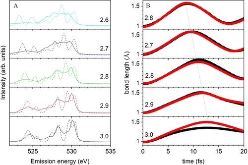
Figure 8(b) shows the time propagation of the OH bond distances depending on the corresponding R(OO) and averaged over the 60 trajectories with different initial conditions. By decreasing R(OO), the time it takes for the OH bonds to reach maximum elongation is reduced and the elongation of the OH bonds becomes larger. We also examined the effect of deviation from tetrahedrality at fixed R(OO) = 2.80 Å by varying the O-O-O angle involving the two H-bond donors (W2 and W5 in Figure 4; see Supplementary information). We found no significant effect on the computed XES from this specific deformation.

3.2. Comparison of sampling schemes

In the present study we also consider the dependence on sampling scheme. Ljungberg et al. [62] investigated the relative importance of sampling the quantum probability distributions in OH distances and proton momenta for a water dimer with reference to a full wave function treatment of the evolving wave packet along the one-dimensional H-bond coordinate. Based on this, and the fact that the zero-point energy is the greatest in the stretch modes, Pettersson and coworkers have focused on sampling the stretch modes only [44,46,62,63,69,70]. Recently one of the authors and coworkers reported theoretical XES spectra of liquid water [60] sampling six modes, i.e. three hindered rotations, the bending, and symmetric and anti-symmetric OH stretching modes. The three translational modes were not included based on the argument that their energy is comparable to the thermal energy and thus should be efficiently sampled in MD simulations. In contrast to in the present work, however, no restriction was applied to ensure that the sampling along the normal modes did not lead to initial energies that exceeded the available zero-point energy; see Supplementary Material. This may have led to exaggerated dynamics, but the experimental trends in terms of effects of temperature and isotope substitution were still qualitatively reproduced. The split, ∼1.6 eV, between the two 1b₁ peaks was too large, which is likely due to the underlying structures from the MD simulation; a similarly too large split was indeed found also when simply summing computed spectra in ref. [64] where a different description of water was used and higher-level QM/MM calculations performed.

Here we compare sampling all nine degrees of freedom, including the translational modes versus only the three internal modes in Figure 9 for the D2A2 and D1A1 model structures. Including also the lower-energy modes in the sampling of the zero-point distribution of positions and momenta does not affect the position and appearance of the high-emission-energy b₁ peak, but does additionally broaden the other features in the spectrum. We attribute this to the additional spread in initial positions of the protons; the contributions in terms of momentum is significantly smaller than that from the internal modes.

Figure 9. Comparison between sampling all nine modes (black) versus only the two stretch modes and the bending vibration (red) for (A) the D2A2 and (B) D1A1 species.

Including the low-frequency (translational and librational) modes in the sampling can clearly be replaced by additional sampling of situations of the underlying molecular dynamics trajectory. However, if one is anyway sampling a particular situation one might as well include all modes. We note that the internal modes show a very small spread in position while that in momentum is large making sampling the momenta of these modes more important than the positions [62]. For the modes involving motion of the whole molecule in the field from its neighbours, the zero-point energy and corresponding spread in momentum is quite small, while the spread in position is larger. We note that including the translational modes requires that the appropriate reduced mass be used as it differs significantly from that of a single proton.

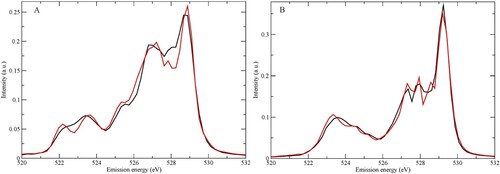
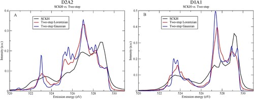
Figure 10 compares three types of convolution schemes applied to the D2A2 and D1A1 species, which are SCKH and two-step with either Lorentzian (equation (4)) or Gaussian (equation (5)) broadening. There are significant differences in the computed spectra, particularly between the SCKH and two-step approaches for both the D2A2 (Figure 10A) and D1A1 (Figure 10B) pentamers. These spectra are all based on the same 60 trajectories and the same computed transitions, but differ in how the spectrum contributions along the CHID were treated when going from the time-domain (spectra at individual CHID time-steps) to an overall spectrum in terms of energy. It is clear that the interference effects as well as the projection of the ground-state vibrational wave function onto the intermediate state potential surface have a very large effect on the intensity distribution in the final computed spectrum.

Figure 10. Comparison between the SCKH and two-step Lorentzian or Gaussian broadenings for (A) D2A2 and (B) D1A1 species.

4. Summary

We investigate core-hole-induced dynamical (CHID) effects on computed XES spectra based on two water pentamers representing D2A2 and D1A1 H-bonded local structures, i.e. tetrahedral and distorted. We show that the characteristic split peaks in the lone-pair b₁ region is due to a combination of an initial-state shift that depends on the H-bonding with the distorted D1A1 pentamer peak at higher energy than that of the D2A2 tetrahedral pentamer; the energy split is further enhanced by the CHID following the creation of the core-hole. This picture of the split being determined by the initial H-bond coordination through both an initial inherent shift and the subsequent dynamics is further established by comparison to higher-level computed spectra for which the summed spectrum agrees with experiment.

Analysing the CHID further we find that for the tetrahedral D2A2 pentamer the dynamics involves both protons moving along the H-bond directions towards the accepting waters, but that on the time-scale of the core-hole life-time there is no dissociation. Rather the protons are reflected back from the accepting water after ∼10 fs due to lack of mechanisms to dissipate the kinetic energy on the relevant time-scale. The emission from the D2A2 model pentamer is thus more atomic-like, as from an O⁻ atom interacting to various degrees with two protons. For the asymmetrically H-bonded D1A1 pentamer, the CHID only involves the H-bonded proton which becomes delocalised between the accepting and donating waters, but also in this case rather as a wave packet being reflected from the accepting water. In this case, the CHID shows a larger spread in the dynamics, i.e. how long it takes for the proton to reach the turning point and be reflected back.

The CHID also involves the H-bond accepting waters where we find a distinct shortening of the O-O distances to the accepting waters. This can be viewed as a natural consequence of the mutual attraction between the proton and the accepting water. Since the accepting waters are not interacting with other waters in these pentamer models, the magnitude of these changes may be exaggerated. However, we observe this tendency also in larger water cluster models as a consequence of CHID. It is furthermore consistent with recent observation of a reduction of O-O distances after excitation of the O-H stretch vibration in liquid water [84]. In this case a smaller effect can be expected as the O-H bond is only slightly elongated, which is also consistent with the longer time-scale for the O-O distance reduction in that case.

We furthermore compare different schemes to sample the initial quantum zero-point distribution, sampling the probability distribution corresponding either only to the internal modes or to all degrees of freedom of the central molecule in the pentamer models. Sampling the soft modes corresponding to translations and librations in addition to the internal modes results in a smoother spectrum, but does not introduce new features or shift in peak positions. However, including these soft modes in the sampling requires that care is taken to not accept distortions that go beyond the classical turning points in the zero-point potential.

We finally compare spectra computed using the semiclassical Kramers-Heisenberg (SCKH) formalism with spectra computed using a two-step approach with either Lorentzian or Gaussian broadening. We find that neglecting the effects of intermediate state interference and the projection on the ground-state vibrational wave function has large effects on the resulting spectra with a significant shift of intensity from the b₁ region to lower energy. The interference effects are a natural consequence of the fact that it cannot be known from which component of the wave packet representing the delocalised proton that the decay actually occurs. We strongly recommend to include in any simulation of XES on H-bonded systems both the effects of CHID with proper sampling of the zero-point probability distribution and the resulting interference effects due to the unresolved intermediate states. An efficient approach to do this is through the here applied SCKH approximation [61–63,69,70,85].

Acknowledgements

We dedicate this contribution to the work and achievements of Nick Besley. Science is not only about the data and papers you publish, but also the mark and inspiration you leave on people. LGMP is grateful for the opportunity to work together with Nick, to meet his family and share mathematical wonders with his gifted daughter. LGMP further acknowledges support from the European Research Council (ERC) Advanced Grant under Project No. 101021166 – GAS-WAT and the Swedish National Research Council (VR) under grant no. 2020-05538. The Swedish National Infrastructure for Computing (SNIC) is acknowledged for providing computational resources at the High Performance Computing Center North (HPC2N). OT would like to thank the Research Center for Computational Science, Okazaki, Japan (Project: 22-IMS-C038), and the Research Institute for Information Technology at Kyushu University, Fukuoka, for computational resources. This work was supported by JSPS KAKENHI Grant Number JP19H05717 (Grant-in-Aid for Scientific Research on Innovative Area: Aquatic Functional Materials).

Disclosure statement

No potential conflict of interest was reported by the author(s).

Additional information

Funding

This work was supported by H2020 European Research Council [grant number 101021166]; JSPS KAKENHI [grant number JP19H05717]; and Vetenskapsrådet: [grant Number 2020-05538].

References

- M.G. Sceats, S.A. Rice and F. Franks, editors, Book Water, a Comprehensive Treatise (Plenum Press, New York, 1982).
- L.G.M. Pettersson, R.H. Henchman and A. Nilsson, Chem. Rev. 116, 7459 (2016). doi:10.1021/acs.chemrev.6b00363
- M.F. Chaplin, Water Structure and Science. (2017). www.lsbu.ac.uk/water/index.html
- P. Gallo, K. Amann-Winkel, C.A. Angell, M.A. Anisimov, F. Caupin, C. Chakravarty, T. Loerting, A.Z. Panagiotopoulos, J. Russo, H. Tanaka, J.A. Sellberg, H.E. Stanley, E. Lascaris, C. Vega, L. Xu and L.G.M. Pettersson, Chem. Rev. 116, 7463 (2016). doi:10.1021/acs.chemrev.5b00750
- P.H. Poole, F. Sciortino, U. Essmann and H.E. Stanley, Nature. 360 (6402), 324 (1992). doi:10.1038/360324a0
- J.W. Biddle, R.S. Singh, E.M. Sparano, F. Ricci, M.A. González, C. Valeriani, J.L.F. Abascal, P.G. Debenedetti, M.A. Anisimov and F. Caupin, J. Chem. Phys. 146, 034502 (2017). doi:10.1063/1.4973546
- V. Holten and M.A. Anisimov, Sci. Reps. 2, 713 (2012); R. S. Singh, J. W. Biddle, P. G. Debenedetti, and M. A. Anisimov, J. Chem. Phys. 144, 144504 (2016). doi:10.1038/srep00713
- J. Russo and H. Tanaka, Nat. Commun. 5, 3556 (2014). doi:10.1038/ncomms4556
- R. Shi, J. Russo and H. Tanaka, J. Chem. Phys. 149, 224502 (2018); H. Tanaka, J. Chem. Phys. 112, 799 (2000). doi:10.1063/1.5055908
- H. Tanaka, European Phys. J. E. 35, 113 (2012). doi:10.1140/epje/i2012-12113-y
- O. Mishima and H.E. Stanley, Nature. 392 (6672), 164 (1998). doi:10.1038/32386
- P.H. Handle, T. Loerting and F. Sciortino, Proc. Natl. Acad. Sci. (USA). 114, 13336 (2017). doi:10.1073/pnas.1700103114
- K.-H. Kim, K. Amann-Winkel, N. Giovambattista, A. Späh, F. Perakis, H. Pathak, M. Ladd Parada, C. Yang, D. Mariedahl, T. Eklund, T.J. Lane, S. You, S. Jeong, M. Weston, J.H. Lee, I. Eom, M. Kim, J. Park, S.H. Chun, P.H. Poole and A. Nilsson, Science. 370, 978 (2020). doi:10.1126/science.abb9385
- F. Perakis, K. Amann-Winkel, F. Lehmkühler, M. Sprung, D. Pettersson, J.A. Sellberg, H. Pathak, A. Späh, F. Cavalca, D. Schlesinger, A. Ricci, A. Jain, B. Massani, F. Aubree, C.J. Benmore, T. Loerting, G. Grübel, L.G.M. Pettersson and A. Nilsson, Proc. Natl. Acad. Sci. (USA). 114, 8193 (2017). doi:10.1073/pnas.1705303114
- J.C. Palmer, F. Martelli, Y. Liu, R. Car, A.Z. Panagiotopoulos and P.G. Debenedetti, Nature. 510, 385 (2014). doi:10.1038/nature13405
- Y. Liu, J.C. Palmer, A.Z. Panagiotopoulos and P.G. Debenedetti, J. Chem. Phys. 137, 214505 (2012). doi:10.1063/1.4769126
- J.C. Palmer, R. Car and P.G. Debenedetti, Faraday Disc. 167, 77 (2013). J. C. Palmer, A. Haji-Akbari, R. S. Singh, F. Martelli, R. Car, A. Z. Panagiotopoulos, and P. G. Debenedetti, J. Chem. Phys. 148, 137101 (2018). doi:10.1039/c3fd00074e
- J.C. Palmer, F. Martelli, Y. Liu, R. Car, A.Z. Panagiotopoulos and P.G. Debenedetti, Nature. 531, E2 (2016). doi:10.1038/nature16540
- J.C. Palmer, P.H. Poole, F. Sciortino and P.G. Debenedetti, Chem. Rev. 118, 9129–9151 (2018). D. Chandler, Nature 531, E1 (2016); D. T. Limmer and D. Chandler, J. Chem. Phys. 135, 134503 (2011); D. T. Limmer and D. Chandler, J. Chem. Phys. 138, 214504 (2013). doi:10.1021/acs.chemrev.8b00228
- D.T. Limmer and D. Chandler, Mol. Phys. 113, 2799 (2015). doi:10.1080/00268976.2015.1029552
- T.A. Kesselring, G. Franzese, S.V. Buldyrev, H.J. Herrmann and H.E. Stanley, Sci. Reps. 2, 474 (2012). T. A. Kesselring, E. Lascaris, G. Franzese, and H. E. Stanley, J. Chem. Phys. 138, 244506 (2013). doi:10.1038/srep00474
- G. Malescio, G. Franzese, G. Pellicane, A. Skibinsky, S.V. Buldyrev and H.E. Stanley, J. Phys.: Cond. Mat. 14, 2193 (2002). doi:10.1088/0953-8984/14/9/308
- K. Stokely, M.G. Mazza, H.E. Stanley and G. Franzese, Proc. Natl. Acad. Sci. (USA). 107, 1301 (2010). doi:10.1073/pnas.0912756107
- H.E. Stanley, Introduction to Phase Transitions and Critical Phenomena (Oxford University Press, New York, 1971).
- K.-H. Kim, A. Späh, H. Pathak, F. Perakis, D. Mariedahl, K. Amann-Winkel, J.A. Sellberg, J.H. Lee, S. Kim, J. Park, K.H. Nam, T. Katayama and A. Nilsson, Science. 358, 1589 (2017). doi:10.1126/science.aap8269
- A. Späh, H. Pathak, K.-H. Kim, F. Perakis, D. Mariedahl, K. Amann-Winkel, J.A. Sellberg, J.H. Lee, S. Kim, J. Park, K.H. Nam, T. Katayama and A. Nilsson, Phys. Chem. Chem. Phys. 21, 26 (2019). doi:10.1039/C8CP05862H
- T.E. Gartner III, K.M. Hunter, E. Lambros, A. Caruso, M. Riera, G.R. Medders, A.Z. Panagiotopoulos, P.G. Debenedetti and F. Paesani, J. Phys. Chem. Lett. 13, 3652 (2022). doi:10.1021/acs.jpclett.2c00567
- C. Huang, K.T. Wikfeldt, T. Tokushima, D. Nordlund, Y. Harada, U. Bergmann, M. Niebuhr, T.M. Weiss, Y. Horikawa, M. Leetmaa, M.P. Ljungberg, O. Takahashi, A. Lenz, L. Ojamäe, A.P. Lyubartsev, S. Shin, L.G.M. Pettersson and A. Nilsson, Proc. Natl. Acad. Sci. (USA). 106, 15214 (2009). doi:10.1073/pnas.0904743106
- A. Nilsson, C. Huang and L.G.M. Pettersson, J. Mol. Liq. 176, 2 (2012). doi:10.1016/j.molliq.2012.06.021
- A. Nilsson and L.G.M. Pettersson, Nat. Commun. 6, 8998 (2015). doi:10.1038/ncomms9998
- H. Tanaka, Phys. Rev. E. 62, 6268 (2000). H. Tanaka, J. Chem. Phys. 153, 130901 (2020). doi:10.1103/PhysRevB.62.6268
- J.R. Scherer, M.K. Go and S. Kint, J. Phys. Chem. 78, 1304 (1974). doi:10.1021/j100606a013
- G.E. Walrafen, J. Chem. Phys. 40, 3249 (1964); G. E. Walrafen, M. S. Hokmabadi, and W.-H. Yang, J. Chem. Phys. 85, 6964 (1986). doi:10.1063/1.1724992
- G.E. Walrafen, W.-H. Yang and Y.C. Chu, ACS Symp. Ser. 676, 287 (1997). doi:10.1021/bk-1997-0676.ch021
- Y. Maréchal, J. Mol. Struct. 1004, 146 (2011). doi:10.1016/j.molstruc.2011.07.054
- Y. Harada, J. Miyawaki, H. Niwa, K. Yamazoe, L.G.M. Pettersson and A. Nilsson, J. Phys. Chem. Lett. 8, 5487 (2017). doi:10.1021/acs.jpclett.7b02060
- Y. Harada, T. Tokushima, Y. Horikawa, O. Takahashi, H. Niwa, M. Kobayashi, M. Oshima, Y. Senba, H. Ohashi, K.T. Wikfeldt, A. Nilsson, L.G.M. Pettersson and S. Shin, Phys. Rev. Lett. 111, 193001 (2013). doi:10.1103/PhysRevLett.111.193001
- P. Wernet, D. Nordlund, U. Bergmann, M. Cavalleri, M. Odelius, H. Ogasawara, LÅ Näslund, T.K. Hirsch, L. Ojamäe, P. Glatzel, L.G.M. Pettersson and A. Nilsson, Science. 304 (5673), 995 (2004). doi:10.1126/science.1096205
- T. Fransson, Y. Harada, N. Kosugi, N.A. Besley, B. Winter, J. Rehr, L.G.M. Pettersson and A. Nilsson, Chem. Rev. 116, 7551 (2016). doi:10.1021/acs.chemrev.5b00672
- A. Nilsson, D. Nordlund, I. Waluyo, N. Huang, H. Ogasawara, S. Kaya, U. Bergmann, L-Å Näslund, H. Öström, P. Wernet, K.J. Andersson, T. Schiros and L.G.M. Pettersson, J. El. Spec. Rel. Phen. 177, 99 (2010). doi:10.1016/j.elspec.2010.02.005
- L.G.M. Pettersson and A. Nilsson, J. Non-Cryst. Solids. 407, 399 (2015). doi:10.1016/j.jnoncrysol.2014.08.026
- T. Tokushima, Y. Horikawa, H. Arai, Y. Harada, O. Takahashi, L.G.M. Pettersson, A. Nilsson and S. Shin, J. Chem. Phys. 136, 044517 (2012). doi:10.1063/1.3678443
- I. Zhovtobriukh, N.A. Besley, T. Fransson, A. Nilsson and L.G.M. Pettersson, J. Chem. Phys. 148, 144507 (2018). doi:10.1063/1.5009457
- A. Nilsson, T. Tokushima, Y. Horikawa, Y. Harada, M.P. Ljungberg, S. Shin and L.G.M. Pettersson, J. Electron. Spectrosc. Relat. Phenom. 188, 84 (2013). T. Tokushima, Y. Harada, Y. Horikawa, O. Takahashi, Y. Senba, H. Ohashi, L. G. M. Pettersson, A. Nilsson, and S. Shin, J. El. Spec. Rel. Phen. 177, 192 (2010). doi:10.1016/j.elspec.2012.09.011
- D. Nordlund, H. Ogasawara, K.J. Andersson, M. Tatarkhanov, M. Salmerón, L.G.M. Pettersson and A. Nilsson, Phys. Rev. B. 80, 233404 (2009). doi:10.1103/PhysRevB.80.233404
- T. Tokushima, Y. Harada, O. Takahashi, Y. Senba, H. Ohashi, L.G.M. Pettersson, A. Nilsson and S. Shin, Chem. Phys. Lett. 460, 387 (2008). doi:10.1016/j.cplett.2008.04.077
- G.N.I. Clark, C.D. Cappa, J.D. Smith, R.J. Saykally and T. Head-Gordon, Mol. Phys. 108, 1415 (2010). doi:10.1080/00268971003762134
- J.D. Smith, C.D. Cappa, K.R. Wilson, R.C. Cohen, P.L. Geissler and R.J. Saykally, Proc. Natl Acad. Sci. (USA). 102, 14171 (2005). doi:10.1073/pnas.0506899102
- J.D. Smith, C.D. Cappa, K.R. Wilson, B.M. Messer, R.C. Cohen and R.J. Saykally, Science. 306, 851 (2004); A. Nilsson, Ph. Wernet, D. Nordlund, U. Bergmann, M. Cavalleri, M. Odelius, H. Ogasawara, L.-Å. Näslund, T. K. Hirsch, L. Ojamäe, P. Glatzel, and L. G. M. Pettersson, Science 308, 793a (2005). doi:10.1126/science.1102560
- M. Odelius, Phys. Rev. B. 79, 144204 (2009); M. Odelius, J. Phys. Chem. A 113, 8176 (2009). doi:10.1103/PhysRevB.79.144204
- V. Vaz da Cruz, F. Gel‘mukhanov, S. Eckert, M. Iannuzzi, E. Ertan, A. Pietzsch, R.C. Couto, J. Niskanen, M. Fondell, M. Dantz, T. Schmitt, X. Lu, D. McNally, R.M. Jay, V. Kimberg, A. Föhlisch and M. Odelius, Nature Comm. 10, 1013 (2019). doi:10.1038/s41467-019-08979-4
- V.W.D. Cruzeiro, A. Wildman, X. Li and F. Paesani, J. Phys. Chem. Lett. 12, 3966 (2021).
- Z. Sun, L. Zheng, M. Chen, M.L. Klein, F. Paesani and X. Wu, Phys. Rev. Lett. 121, 137401 (2018); F. Tang, Z. Li, C. Zhang, S. G. Louie, R. Car, D. Y. Qiu, and X. Wu, Proc. Natl. Acad. Sci. (USA) 119, e2201258119 (2022). doi:10.1103/PhysRevLett.121.137401
- O. Fuchs, M. Zharnikov, L. Weinhardt, M. Blum, M. Weigand, Y. Zubavichus, M. Bär, F. Maier, J.D. Denlinger, C. Heske, M. Grunze and E. Umbach, Phys. Rev. Lett. 100, 027801 (2008). doi:10.1103/PhysRevLett.100.027801
- O. Fuchs, M. Zharnikov, L. Weinhardt, M. Blum, M. Weigand, Y. Zubavichus, M. Bär, F. Maier, J.D. Denlinger, C. Heske, M. Grunze and E. Umbach, Phys. Rev. Lett. 100, 249802 (2008). doi:10.1103/PhysRevLett.100.249802
- J. Niskanen, M. Fondell, C.J. Sahle, S. Eckert, R.M. Jay, K. Gilmore, A. Pietzsch, M. Dantz, X. Lu, D. McNally, T. Schmitt, V. Vaz da Cruz, V. Kimberg, F. Gel‘mukhanov and A. Föhlisch, Proc. Natl. Acad. Sci. (USA). 116, 17158 (2019); J. Niskanen, M. Fondell, C. J. Sahle, S. Eckert, R. M. Jay, K. Gilmore, A. Pietzsch, M. Dantz, X. Lu, D. E. McNally, T. Schmitt, V. Vaz da Cruz, V. Kimberg, F. Gel‘mukhanov, and A. Föhlisch, Proc. Natl. Acad. Sci. (USA) 116, 4058 (2019). doi:10.1073/pnas.1909551116
- L.G.M. Pettersson, T. Tokushima, Y. Harada, O. Takahashi, S. Shin and A. Nilsson, Phys. Rev. Lett. 100, 249801 (2008). doi:10.1103/PhysRevLett.100.249801
- L.G.M. Pettersson, Y. Harada and A. Nilsson, Proc. Natl. Acad. Sci. (USA). 116, 17156 (2019). doi:10.1073/pnas.1905756116
- K. Yamazoe, J. Miyawaki, H. Niwa, A. Nilsson and Y. Harada, J. Chem. Phys. 150, 204201 (2019). doi:10.1063/1.5081886
- O. Takahashi, R. Yamamura, T. Tokushima and Y. Harada, Phys. Rev. Lett. 128, 086002 (2022). doi:10.1103/PhysRevLett.128.086002
- M.P. Ljungberg, Semi-Classical Kramers-Heisenberg code download (https://github.com/mathiasljungberg/sckh, GitHub, 2018).
- M.P. Ljungberg, A. Nilsson and L.G.M. Pettersson, Phys. Rev. B. 82, 245115 (2010). doi:10.1103/PhysRevB.82.245115
- M.P. Ljungberg, L.G.M. Pettersson and A. Nilsson, J. Chem. Phys. 134, 044513 (2011). doi:10.1063/1.3533956
- L.G.M. Pettersson and O. Takahashi, J. Non-Crystalline Solids: X. 14, 10087 (2022).
- N.A. Besley, Chem. Phys. Lett. 542, 42 (2012). doi:10.1016/j.cplett.2012.05.059
- L.B. Skinner, C. Huang, D. Schlesinger, L.G.M. Pettersson, A. Nilsson and C.J. Benmore, J. Chem. Phys. 138, 074506 (2013). doi:10.1063/1.4790861
- A. Goto, T. Hondoh and S. Mae, J. Chem. Phys. 93, 1412 (1990). doi:10.1063/1.459150
- F.K. Gel‘mukhanov, L.N. Mazalov and A.V. Kondratenko, Chem. Phys. Lett. 46, 133 (1977). doi:10.1016/0009-2614(77)85180-4
- M.P. Ljungberg, I. Zhovtobriukh, O. Takahashi and L.G.M. Pettersson, J. Chem. Phys. 146, 134506 (2017). doi:10.1063/1.4979656
- O. Takahashi, M.P. Ljungberg and L.G.M. Pettersson, J. Phys. Chem. B. 121, 11163–11168 (2017). doi:10.1021/acs.jpcb.7b09262
- M. Neeb, J.E. Rubensson, M. Biermann and W. Eberhardt, J. El. Spec. Rel. Phen. 67 (2), 261 (1994). doi:10.1016/0368-2048(93)02050-V
- R. Sankari, M. Ehara, H. Nakatsuji, Y. Senba, K. Hosokawa, H. Yoshida, A. De Fanis, Y. Tamenori, S. Aksela and K. Ueda, Chem. Phys. Lett. 380, 647 (2003). doi:10.1016/j.cplett.2003.08.108
- A. Föhlisch, J. Hasselström, P. Bennich, N. Wassdahl, O. Karis, A. Nilsson, L. Triguero, M. Nyberg and L.G.M. Pettersson, Phys. Rev. B. 61, 16229 (2000). doi:10.1103/PhysRevB.61.16229
- A.M. Koster, G. Geudtner, A. Alvarez-Ibarra, P. Calaminici, M.E. Casida, J. Carmona-Espindola, F.A. Delesma, R. Delgado Venegas, V.D. Dominguez, R. Flores-Moreno, G.U. Gamboa, A. Goursot, T. Heine, A. Ipatov, A. de la Lande, F. Janetzko, J. Martin del Campo, N. Pedroza Montero, L.G.M. Pettersson, D. Mejia-Rodriguez, J. Reveles, J. Vasquez-Perez, A. Vela, B. Zuniga-Gutierrez and D.R. Salahub, deMon2k (The deMon Developers) (Cinvestav, México, Mexico City, 2020). See also www.demon-software.com.
- J.P. Perdew, K. Burke and M. Ernzerhof, Phys. Rev. Lett. 77, 3865 (1996). doi:10.1103/PhysRevLett.77.3865
- W. Kutzelnigg, U. Fleischer and M. Schindler, NMR-Basic Principles and Progress (Springer Verlag, Heidelberg, 1990).
- M.J. Frisch, G.W. Trucks, H.B. Schlegel, G.E. Scuseria, M.A. Robb, J.R. Cheeseman, G. Scalmani, V. Barone, G.A. Petersson, H. Nakatsuji, X. Li, M. Caricato, A.V. Marenich, J. Bloino, B.G. Janesko, R. Gomperts, B. Mennucci, H.P. Hratchian, J.V. Ortiz, A.F. Izmaylov, J.L. Sonnenberg, D. Williams-Young, F. Ding, F. Lipparini, F. Egidi, J. Goings, B. Peng, A. Petrone, T. Henderson, D. Ranasinghe, V.G. Zakrzewski, J. Gao, N. Rega, G. Zheng, W. Liang, M. Hada, M. Ehara, K. Toyota, R. Fukuda, J. Hasegawa, M. Ishida, T. Nakajima, Y. Honda, O. Kitao, H. Nakai, T. Vreven, K. Throssell, J.A. Montgomery, Jr., J.E. Peralta, F. Ogliaro, M.J. Bearpark, J.J. Heyd, E.N. Brothers, K.N. Kudin, V.N. Staroverov, T.A. Keith, R. Kobayashi, J. Normand, K. Raghavachari, A.P. Rendell, J.C. Burant, S.S. Iyengar, J. Tomasi, M. Cossi, J.M. Millam, M. Klene, C. Adamo, R. Cammi, J.W. Ochterski, R.L. Martin, K. Morokuma, O. Farkas, J.B. Foresman and D.J. Fox, Gaussian 16, Revision B.01 (Gaussian, Inc., Wallingford CT, 2016).
- L.G.M. Pettersson and O. Takahashi, Theor. Chem. Acc. 140, 162 (2021). doi:10.1007/s00214-021-02859-1
- M. Leetmaa, K.T. Wikfeldt and L.G.M. Pettersson, J. Phys. Cond. Mat. 22, 135001 (2010). doi:10.1088/0953-8984/22/13/135001
- M. Odelius, H. Ogasawara, D. Nordlund, O. Fuchs, L. Weinhardt, F. Maier, E. Umbach, C. Heske, Y. Zubavichus, M. Grunze, J.D. Denlinger, L.G.M. Pettersson and A. Nilsson, Phys. Rev. Lett. 94 (22), 227401 (2005). doi:10.1103/PhysRevLett.94.227401
- M. Cavalleri, H. Ogasawara, L.G.M. Pettersson and A. Nilsson, Chem. Phys. Lett. 364, 363 (2002). doi:10.1016/S0009-2614(02)00890-4
- D. Nordlund, H. Ogasawara, H. Bluhm, O. Takahashi, M. Odelius, M. Nagasono, L.G.M. Pettersson and A. Nilsson, Phys. Rev. Lett. 99, 217406 (2007). doi:10.1103/PhysRevLett.99.217406
- U. Bergmann, A. Di Cicco, P. Wernet, E. Principi, P. Glatzel and A. Nilsson, J. Chem. Phys. 127, 174504 (2007); U. Bergmann, A. Di Cicco, Ph. Wernet, E. Principi, P. Glatzel, and A. Nilsson, J. Chem. Phys. 128, 089902 (2008); K. T. Wikfeldt, M. Leetmaa, A. Mace, A. Nilsson, and L. G. M. Pettersson, J. Chem. Phys. 132, 104513 (2010). doi:10.1063/1.2784123
- J. Yang, R. Dettori, J.P.F. Nunes, N.H. List, E. Biasin, M. Centurion, Z. Chen, A.A. Cordones, D.P. DePonte, T.F. Heinz, M.E. Kozina, K. Ledbetter, M.-F. Lin, A.M. Lindenberg, M. Mo, A. Nilsson, X. Shen, T.J.A. Wolf, D. Donadio, K.J. Gaffney, T.J. Martinez and X. Wang, Nature. 596, 531 (2021). doi:10.1038/s41586-021-03793-9
- M.P. Ljungberg, Phys. Rev. B. 96, 214302 (2017). doi:10.1103/PhysRevB.96.214302