Derivation of the Casimir contribution to the binding potential for 3D wetting

ABSTRACT

The renormalisation group theory of critical and tri-critical wetting transitions in three-dimensional systems with short-ranged forces, based on analysis of an effective Hamiltonian with an interfacial binding potential $w\left(\ell \right)$, predicts very strong non-universal critical singularities. These, however, have famously not been observed in extensive Monte Carlo simulations of the transitions in the simple cubic Ising model. Here, we show that previous treatments have missed an entropic, or low-temperature Casimir, contribution to the binding potential, arising from the many different microscopic configurations which correspond to a given interfacial one. We derive the full binding potential, including the Casimir correction term, starting from a microscopic Landau–Ginzburg–Wilson Hamiltonian, using a continuum transfer-matrix (path-integral) method. This is illustrated first in one dimension before generalising to arbitrary dimension. The Casimir contribution is qualitatively different for first-order, critical and tri-critical wetting transitions and substantially alters previous predictions for critical singularities bringing them much closer to the simulation results.

GRAPHICAL ABSTRACT

KEYWORDS:

• Wetting
• fluctuations
• Casimir forces

1. Introduction

A long-standing problem in the theory of phase transitions and fluid interfacial phenomena concerns the nature of the critical wetting transition (for general reviews of wetting see [1–4]) in three-dimensional systems with short-ranged forces where predictions of very strongly non-universal critical singularities, based on renormalisation group (RG) studies of an effective interfacial Hamiltonian [5–7], are not supported by Monte Carlo simulation studies of the transition in the simple cubic Ising model [8–13]. Some progress has been made and have drawn the controversy into sharper focus. For example, it is not the case, as was originally thought, that the Ising model simulations only reveal mean-field-like behaviour but rather that non-classical behaviour is present, and is observable in surface thermodynamic quantities and cumulant averages, but not in any way to the degree expected – for example, the correlation length critical exponent is measured to be ${\nu }_{\parallel }\approx 2$ [12,13] compared with the theoretical expectation ${\nu }_{\parallel }\approx 3.7$ [6,7,14,15] (with the mean-field result, which ignores interfacial fluctuation effects, corresponding to ${\nu }_{\parallel }=1$ for comparison [16]). In addition, it is now understood that the critical wetting transition is not fluctuation-induced first-order, as was once speculated [17–19], because the effective Hamiltonian contains non-local interfacial interactions which entirely preclude this possibility [20–23]. Nevertheless, nearly four decades on from the original RG studies, the suspicion remains that something fundamental has been missing in the theoretical description of interfacial fluctuation effects at wetting transitions which come to light at the marginal dimension d = 3.

The general fluctuation theory of wetting transitions is based, primarily, on studies of interfacial Hamiltonians which take the simple form [3,24] (1) $\begin{array}{r}{H}_I\left[\ell \right]=\int \mathrm{d}\mathbf{x}\left(\frac{\gamma }{2}\right(\mathrm{\nabla }\ell {)}^2+w\left(\ell \right)),\end{array}$(1) where $\ell \left(\mathbf{x}\mathbf{\right)}$ is a mesoscopic collective coordinate representing the local height/thickness of a layer of liquid adsorbed at a wall-gas interface with $\mathbf{x}$ the parallel displacement. The first term in the Hamiltonian contains the surface tension γ of the liquid-gas interface and serves simply to resist fluctuations which increase the interfacial area as the interface unbinds from the wall. The second term is the binding potential $w\left(\ell \right)$ which corresponds to the energy cost of a wetting layer of liquid (say) of uniform thickness ℓ. The local Hamiltonian (1(1) $\begin{array}{r}{H}_I\left[\ell \right]=\int \mathrm{d}\mathbf{x}\left(\frac{\gamma }{2}\right(\mathrm{\nabla }\ell {)}^2+w\left(\ell \right)),\end{array}$(1) ) is an approximation to a more general interfacial model in which the tension γ multiplies the full interfacial area (not just the leading order gradient term) and where the function $w\left(\ell \right)$ is replaced with $W\left[\ell \right]$ which is a functional of the interface (and wall) shape. The binding potential function $w\left(\ell \right)$ then corresponds to the specific case when the wall and interface are both flat and parallel to each other, which suffices for many purposes. We shall return to this more general Hamiltonian at the end of our paper.

The form of the binding potential $w\left(\ell \right)$ in the local Hamiltonian (1(1) $\begin{array}{r}{H}_I\left[\ell \right]=\int \mathrm{d}\mathbf{x}\left(\frac{\gamma }{2}\right(\mathrm{\nabla }\ell {)}^2+w\left(\ell \right)),\end{array}$(1) ) depends on the range of the intermolecular interactions and is well understood for systems with dispersion interactions, for which fluctuation effects are not particularly important [25]. However, in a recent paper [26], we showed that the form of $w\left(\ell \right)$ that has been used in studies of critical wetting (and also tri-critical and first-order wetting transitions) in systems with short-ranged forces is incorrect since it has missed an important entropic or thermal Casimir contribution arising from the many microscopic configurations that correspond to a given interfacial one. This contribution is entirely absent in traditional mean-field treatments of wetting which have been used previously to justify and derive the interfacial model. Consequently, all previous approaches have, in fact, only identified the classical or mean-field contribution $w_{\mathrm{M}\mathrm{F}}\left(\ell \right)$ to the binding potential function, which more correctly is written (2) $\begin{array}{r}w\left(\ell \right)=w_{\mathrm{M}\mathrm{F}}\left(\ell \right)+w_C\left(\ell \right)\end{array}$(2) containing an additive Casimir correction. Including the Casimir contribution changes, radically, predictions for critical singularities at tri-critical and first-order wetting transitions and brings the RG predictions for critical wetting into very close agreement with the results of the Ising model simulations.

In this paper, we provide comprehensive details of how the correct binding potential, including the Casimir contribution, may be calculated rigorously and systematically from an underlying Landau–Ginzburg–Wilson Hamiltonian by performing a (constrained) trace over microscopic configurations. The method that we follow here is based on the generalisation to higher dimensions of an elegant transfer matrix or path integral technique, familiar from related studies in 2D, which maps the evaluation of the partition function onto elementary quantum mechanics [27,28]. This method was also used to derive the Casimir-like forces induced by director fluctuations in nematic liquid crystals confined between rigid walls [29]. However, instead of using the path integral technique to evaluate the partition function (and equilibrium observables) of the interfacial model in 2D, here we use the method to determine a constrained partition function for the microscopic Landau–Ginzburg–Wilson Hamiltonian and hence derive the binding potential $w\left(\ell \right)$ for the 3D interfacial model itself. This very clearly reveals the origin of the mean-field (classical) and Casimir (non-classical), contributions to $w\left(\ell \right)$ and identifies that in 3D the Casimir term is (3) $\begin{array}{r}{w}_C\left(\ell \right)=\frac{k_{B}T}{4\pi }{\int }_0^{\mathrm{\infty }}\mathrm{d}qq\ln (1-\frac{g+{\kappa }_q}{g-{\kappa }_q}{\mathrm{e}}^{-2{\kappa }_q\ell }),\end{array}$(3) where g is the surface enhancement and ${\kappa }_q=\sqrt{{\kappa }^2+q^2}$ with $\kappa =1/\xi$ the inverse of the bulk correlation length and q the modulus of the transverse wavenumber vector. This is the central result of our paper. We show how the Casimir term competes with the usual mean-field contribution to the binding potential, maybe attractive or repulsive depending on the boundary conditions, and is qualitatively different for critical and first-order wetting. The impact of the Casimir term on RG studies is outlined in the discussion as well as the connection with the more general non-local Hamiltonian and the diagrammatic representation of the Casimir contribution, $W_C\left[\ell \right]$, to the binding potential functional.

2. The LGW Hamiltonian and mean-field binding potential

The starting point for our study is the standard Landau–Ginzburg–Wilson (LGW) Hamiltonian for adsorption at a planar wall, of infinite area $L_{\parallel }^{d-1}$ situated in the z = 0 plane, based on a scalar, magnetisation-like, order parameter (4) $\begin{array}{r}{H}_{\mathrm{L}\mathrm{G}\mathrm{W}}\left[m\right]=\int \mathrm{d}\mathbf{r}\left(\frac{1}{2}\right(\mathbf{\nabla }m{)}^2+f\left(m\right))+{\int }_{\mathcal{S}}\mathrm{d}\mathbf{x}{f}_1\left(m\right(\mathbf{x}\left)\right).\end{array}$(4) Here, $f\left(m\right)$ is a double well potential modelling bulk phase coexistence below a critical temperature $T_c$. We assume an Ising symmetry and denote the spontaneous magnetisation $m_0$ and let $\kappa =1/\xi$ be the inverse of the bulk correlation length. We suppose that the bulk magnetic field $h=0^{-}$ so that, far from the wall, the bulk phase has equilibrium magnetisation $-m_0$ (which we may think of as a ‘gas’, in a fluid language). The surface potential $f_1$ couples to the local surface magnetisation $m\left(\mathbf{x}\right)$, for which we take the standard form (5) $\begin{array}{r}{f}_1=-\frac{g}{2}{m}^2-h_{1}m,\end{array}$(5) where g<0 is the surface enhancement pertinent for wetting by a liquid and $h_1>0$ is the surface field which induces a wetting layer of net positive magnetisation (‘liquid’, in a fluid language). Alternatively, it is convenient to complete the square and write this as (6) $\begin{array}{r}{f}_1=-\frac{g}{2}(m-m_s{)}^2,\end{array}$(6) where $m_s=-h_1/g$ is the preferred magnetisation at the wall. The binding potential $w\left(\ell \right)$ appearing in the local interfacial Hamiltonian is identified as follows [30]: First, we define a constrained partition function (7) $\begin{array}{r}\mathcal{Z}(\ell ;L,L_{\parallel })=\int D{m}^{\prime }{\mathrm{e}}^{-\text{β}{H}_{\mathrm{L}\mathrm{G}\mathrm{W}}\left[m\right]},\end{array}$(7) where L is the system size perpendicular to the wall and the prime indicates that the functional integral only contains magnetisation profiles that correspond to a wetting layer of uniform thickness ℓ. We adopt the crossing criterion definition of the wetting layer thickness which, for a planar wetting layer, means that the value of the magnetisation is fixed to m = 0 at a distance $z=\ell$ from the wall [30].

From this partition function, we then defined a constrained free-energy [30], per unit area, via (8) $\begin{array}{r}F\left(\ell \right)=-\frac{k_{B}T}{L_{\parallel }^{d-1}}\ln \mathcal{Z}(\ell ;L,L_{\parallel }),\end{array}$(8) which we write as (9) $\begin{array}{r}F\left(\ell \right)=w\left(\ell \right)+L{f}_b+\gamma +{\gamma }_{wl}.\end{array}$(9) The dependence on the wetting layer thickness ℓ formally identifies the binding potential $w\left(\ell \right)$ which, for $h=0^{-},$ vanishes as $\ell \to \mathrm{\infty }$. The constrained free-energy $F\left(\ell \right)$ also contains the surface tensions of the liquid-gas and wall-liquid interfaces and also an extensive bulk contribution which is proportional to the system size L, which is always taken as infinite, with $f_b$ denoting the appropriate bulk free-energy density. These are all ℓ independent terms.

In evaluating the constrained partition function, it is now usual to make the saddle point or mean-field (MF) approximation, that bulk fluctuations can be entirely ignored. With this assumption there is only a single contribution to the partition function sum coming from the magnetisation profile $m_{\pi }(z;\ell ),$ which minimises the LGW Hamiltonian subject to the crossing criterion constraint $m_{\pi }(\ell ;\ell )=0$ (see Figure 1). This identifies the MF constrained free-energy as (10) $\begin{array}{r}{F}_{\mathrm{M}\mathrm{F}}\left(\ell \right)=H_{\mathrm{L}\mathrm{G}\mathrm{W}}\left[m_{\pi }\right],\end{array}$(10) where in this case the bulk free-energy density is simply $f_b=f(-m_0)$ and the values of γ and ${\gamma }_{wl}$ are known from standard square-gradient theory.

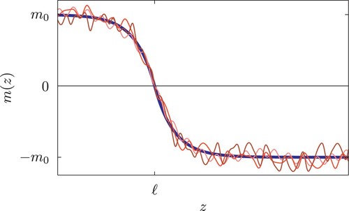
Figure 1. Schematic illustration of the constrained MF magnetisation profile $m_{\pi }(z;\ell )$ (smooth, thick, blue line) and small fluctuations around it (wiggly, thin, red lines) which also satisfy the crossing criterion that m = 0 at $z=\ell$. The MF profile is unique and determines the MF contribution to the binding potential $w_{\mathrm{M}\mathrm{F}}\left(\ell \right)$, while the myriad of distinct, small fluctuations, about $m_{\pi }(z;\ell )$, which all correspond to the same interfacial configuration determines the additive entropic, or Casimir, contribution $w_C\left(\ell \right)$.

This recipe for evaluating the binding potential can be done explicitly within the reliable double-parabola (DP) approximation for the bulk potential (11) $\begin{array}{r}f\left(m\right)=\frac{{\kappa }^2}{2}(|m|-m_0{)}^2,\end{array}$(11) allowing us to determine the mean-field binding potential analytically. For the case of fixed boundary conditions, where we fix the value of the surface magnetisation $m\left(0\right)$ to $m_s$ (equivalent to the limit of $-g\to \mathrm{\infty }$), this determines that $f_b=0$, $\gamma =\kappa m_0^2$, ${\gamma }_{wl}=\kappa \delta m_s^2/2$ and that the MF binding potential is given by (12) $\begin{array}{rl}{w}_{\mathrm{M}\mathrm{F}}\left(\ell \right)& =2\kappa \delta m_s{m}_0\frac{{\mathrm{e}}^{-\kappa \ell }}{1-{\mathrm{e}}^{-2\kappa \ell }}\\ & +\kappa (m_0^2+\delta m_s^2)\frac{{\mathrm{e}}^{-2\kappa \ell }}{1-{\mathrm{e}}^{-2\kappa \ell }},\end{array}$(12) or equivalently (13) $\begin{array}{r}{w}_{\mathrm{M}\mathrm{F}}\left(\ell \right)=\frac{\kappa \delta m_s{m}_0}{\sinh \kappa \ell }+\frac{\kappa (m_0^2+\delta m_s^2)}{2}(\coth \kappa \ell -1),\end{array}$(13) where $\delta m_s=m_s-m_0$. This model only shows continuous (critical) wetting at mean-field level and beyond. More generally, for finite values of the surface enhancement, the binding potential similarly has an expansion in terms of exponentially decaying contributions (14) $\begin{array}{r}{w}_{\mathrm{M}\mathrm{F}}\left(\ell \right)=a{\mathrm{e}}^{-\kappa \ell }+b{\mathrm{e}}^{-2\kappa \ell }+\cdots ,\end{array}$(14) which is believed to be robust beyond the DP approximation and where the next relevant term is proportional to ${\mathrm{e}}^{-3\kappa \ell }$. The coefficients appearing in this expression are (15) $\begin{array}{r}a=-\gamma \frac{2gt}{g-\kappa },b=\gamma \frac{g+\kappa }{g-\kappa },\end{array}$(15) where, as earlier $\gamma =\kappa m_0^2$ is the DP surface tension and $t=(m_0-m_s)/m_0$ is the temperature-like scaling field appropriate for critical wetting (for which b>0) and tri-critical wetting (for which b = 0). The MF binding potential obviously encodes the underlying MF singularities that occur at wetting transitions and has been the basis for RG studies of interfacial fluctuation based on the effective Hamiltonian (12(12) $\begin{array}{rl}{w}_{\mathrm{M}\mathrm{F}}\left(\ell \right)& =2\kappa \delta m_s{m}_0\frac{{\mathrm{e}}^{-\kappa \ell }}{1-{\mathrm{e}}^{-2\kappa \ell }}\\ & +\kappa (m_0^2+\delta m_s^2)\frac{{\mathrm{e}}^{-2\kappa \ell }}{1-{\mathrm{e}}^{-2\kappa \ell }},\end{array}$(12) ) [6,7].

In the next sections, we shall show, however, that the saddle point evaluation of the constrained partition function misses some important contributions arising from small bulk-like fluctuations about the MF configuration $m_{\pi }(z;\ell )$ which can compete with the exponential terms in the MF contribution.

3. Transfer-matrix formalism for the 1D case

Here, we employ a transfer matrix approach in order to derive the constrained partition function, and hence identify $F\left(\ell \right)$ and the desired binding potential $w\left(\ell \right)$, for the DP potential without having to make the MF approximation (10(10) $\begin{array}{r}{F}_{\mathrm{M}\mathrm{F}}\left(\ell \right)=H_{\mathrm{L}\mathrm{G}\mathrm{W}}\left[m_{\pi }\right],\end{array}$(10) ). We do this in one dimension first before explaining how this readily generalises to higher dimensions. The calculation in one dimension also allows us to give a novel ‘quantum mechanical’ interpretation to the exponential decay of the binding potential, together with the values of the coefficient a and b, at and beyond MF level. The idea is to split the LGW Hamiltonian into two subdomains, one of them corresponding to the liquid region, where $0<z<\ell$, for which $f\left(m\right)={\kappa }^2(m-m_0{)}^2/2$, and the gas region, $\ell <z<L$, where $f\left(m\right)={\kappa }^2(m+m_0{)}^2/2$ prior to taking the thermodynamic limit $L\to \mathrm{\infty }$. Thus, we write (16) $\begin{array}{r}{H}_{\mathrm{L}\mathrm{G}\mathrm{W}}\left[m\right]=H_{\mathrm{L}\mathrm{G}\mathrm{W}}^{\mathrm{l}\mathrm{i}\mathrm{q}}\left[m\right]+H_{\mathrm{L}\mathrm{G}\mathrm{W}}^{\mathrm{g}\mathrm{a}\mathrm{s}}\left[m\right],\end{array}$(16) where (17) $\begin{array}{rl}{H}_{\mathrm{L}\mathrm{G}\mathrm{W}}^{\mathrm{l}\mathrm{i}\mathrm{q}}& =-\frac{g}{2}{\left(m\right(0)-m_s)}^2\\ & +{\int }_0^{\ell }\mathrm{d}z[\frac{1}{2}{\left(\frac{\mathrm{d}m}{\mathrm{d}x}\right)}^2+\frac{{\kappa }^2}{2}(m-m_0{)}^2]\end{array}$(17) and (18) $\begin{array}{r}{H}_{\mathrm{L}\mathrm{G}\mathrm{W}}^{\mathrm{g}\mathrm{a}\mathrm{s}}={\int }_{\ell }^L\mathrm{d}z[\frac{1}{2}{\left(\frac{\mathrm{d}m}{\mathrm{d}x}\right)}^2+\frac{{\kappa }^2}{2}(m+m_0{)}^2].\end{array}$(18) The crossing criterion, $m\left(\ell \right)=0$, imposed at the interface implies that the spatial regions $z<\ell$ and z<L are independent, allowing us to factorise the global path integral $\mathcal{Z}(\ell ;L)={\mathrm{e}}^{-\text{β}F\left(\ell \right)}$ into sums over two field configurations. As before, we start our discussion with the situation in which the magnetisation at the wall is fixed, corresponding to the limit $g\to -\mathrm{\infty }$ and $m\left(0\right)=m_s$, which gave rise to the MF binding potential (12(12) $\begin{array}{rl}{w}_{\mathrm{M}\mathrm{F}}\left(\ell \right)& =2\kappa \delta m_s{m}_0\frac{{\mathrm{e}}^{-\kappa \ell }}{1-{\mathrm{e}}^{-2\kappa \ell }}\\ & +\kappa (m_0^2+\delta m_s^2)\frac{{\mathrm{e}}^{-2\kappa \ell }}{1-{\mathrm{e}}^{-2\kappa \ell }},\end{array}$(12) ). Under these circumstances, we can write (19) $\begin{array}{r}{\mathrm{e}}^{-\text{β}F\left(\ell \right)}=\mathcal{Z}(\delta m_s,0|-m_0,\ell \left)\mathcal{Z}\right(m_0,\ell |0,L)\end{array}$(19) where, as earlier, $\delta m_s=m_s-m_0$. Here, $\mathcal{Z}({\varphi }_1,{\ell }_1|{\varphi }_2,{\ell }_2)$ is the partition function defined for the Gaussian Hamiltonian (20) $\begin{array}{r}H={\int }_{{\ell }_1}^{{\ell }_2}\mathrm{d}x[\frac{1}{2}{\left(\frac{\mathrm{d}\varphi \left(x\right)}{\mathrm{d}x}\right)}^2+\frac{{\kappa }^2}{2}\varphi (x{)}^2],\end{array}$(20) with a field $\varphi \left(x\right)$ which is fixed to the values ${\varphi }_1$ and ${\varphi }_2$ at positions ${\ell }_1$ and ${\ell }_2,$ respectively. Elementary path integral techniques [27,28] imply that this has the spectral decomposition (21) $\begin{array}{r}\mathcal{Z}({\varphi }_1,{\ell }_1|{\varphi }_2,{\ell }_2)=\sum _{n=0}^{\mathrm{\infty }}{\mathrm{\Psi }}_n^{\ast }({\varphi }_1\left){\mathrm{\Psi }}_n\right({\varphi }_2){\mathrm{e}}^{-\text{β}{E}_n({\ell }_2-{\ell }_1)},\end{array}$(21) where the ${\mathrm{\Psi }}_n\left(\varphi \right)$ are simply the normalised eigenfunctions of the Schrödinger equation for the simple harmonic oscillator: (22) $\begin{array}{r}-\frac{1}{2{\text{β}}^2}\frac{{\mathrm{d}}^2}{\mathrm{d}{\varphi }^2}{\mathrm{\Psi }}_n\left(\varphi \right)+\frac{{\kappa }^2}{2}{\varphi }^2{\mathrm{\Psi }}_n\left(\varphi \right)=E_n{\mathrm{\Psi }}_n\left(\varphi \right).\end{array}$(22) These, of course, have discrete energy levels (23) $\begin{array}{r}\text{β}{E}_n=(n+\frac{1}{2})\kappa ,\end{array}$(23) with corresponding wavefunctions (24) $\begin{array}{r}{\mathrm{\Psi }}_n\left(\varphi \right)=\frac{1}{\sqrt{2^{n}n!}}{\left(\frac{\text{β}\kappa }{\pi }\right)}^{1/4}{H}_n\left(\sqrt{\text{β}\kappa }\varphi \right){\mathrm{e}}^{-\text{β}\kappa {\varphi }^2/2},\end{array}$(24) where $H_n\left(x\right)$ are Hermite polynomials. The partition function $\mathcal{Z}({\varphi }_1,{\ell }_1|{\varphi }_2,{\ell }_2)$ can be evaluated in closed form using Mehler's identity (25) $\begin{array}{rl}& \sum _{n=0}^{\mathrm{\infty }}\frac{(\rho /2{)}^n}{n!}{H}_n\left(x\right)H_n\left(y\right){\mathrm{e}}^{-\frac{x^2+y^2}{2}}\\ & =\frac{1}{\sqrt{1-{\rho }^2}}\exp [-\frac{{\rho }^2(x^2+y^2)-2\rho xy}{1-{\rho }^2}],\end{array}$(25) yielding (26) $\begin{array}{rl}& \mathcal{Z}({\varphi }_1,{\ell }_1|{\varphi }_2,{\ell }_2)\\ & =\sqrt{\frac{\text{β}\kappa }{2\pi \sinh \kappa {\ell }_{21}}}\\ & \times \exp (\frac{\text{β}\kappa {\varphi }_1{\varphi }_2}{\sinh \kappa {\ell }_{21}}-\frac{\text{β}\kappa ({\varphi }_1^2+{\varphi }_2^2)}{2}\coth \kappa {\ell }_{21}),\end{array}$(26) where ${\ell }_{21}={\ell }_2-{\ell }_1$. This result can be alternatively obtained from a discretised version of the LGW Hamiltonian Equation (20(20) $\begin{array}{r}H={\int }_{{\ell }_1}^{{\ell }_2}\mathrm{d}x[\frac{1}{2}{\left(\frac{\mathrm{d}\varphi \left(x\right)}{\mathrm{d}x}\right)}^2+\frac{{\kappa }^2}{2}\varphi (x{)}^2],\end{array}$(20) ), see the Appendix for further details. Substituting into (19(19) $\begin{array}{r}{\mathrm{e}}^{-\text{β}F\left(\ell \right)}=\mathcal{Z}(\delta m_s,0|-m_0,\ell \left)\mathcal{Z}\right(m_0,\ell |0,L)\end{array}$(19) ) then identifies that the constrained free energy is exactly given by (27) $\begin{array}{r}{\mathrm{e}}^{-\text{β}F\left(\ell \right)}=\frac{\text{β}\kappa }{2\pi }\frac{{\mathrm{e}}^{-\text{β}{F}_{\mathrm{M}\mathrm{F}}\left(\ell \right)}}{\sqrt{\sinh \kappa \ell \sinh \kappa (L-\ell )}},\end{array}$(27) where $F_{\mathrm{M}\mathrm{F}}$ is the MF free energy given by (28) $\begin{array}{rl}{F}_{\mathrm{M}\mathrm{F}}\left(\ell \right)& =\kappa m_0^2+\frac{\kappa \delta m_s^2}{2}+\frac{\kappa m_0\delta m_s}{\sinh \kappa \ell }\\ & +\frac{\kappa (m_0^2+\delta m_s^2)}{2}(\coth \kappa \ell -1)\\ & +\frac{\kappa m_0^2}{2}(\coth \kappa (L-\ell )-1).\end{array}$(28) We can recognise that, if we neglect terms which decay as ${\mathrm{e}}^{-2\kappa L}$, the terms appearing in the r.h.s. of Equation (28(28) $\begin{array}{rl}{F}_{\mathrm{M}\mathrm{F}}\left(\ell \right)& =\kappa m_0^2+\frac{\kappa \delta m_s^2}{2}+\frac{\kappa m_0\delta m_s}{\sinh \kappa \ell }\\ & +\frac{\kappa (m_0^2+\delta m_s^2)}{2}(\coth \kappa \ell -1)\\ & +\frac{\kappa m_0^2}{2}(\coth \kappa (L-\ell )-1).\end{array}$(28) ) are non-other than the MF results for γ, ${\gamma }_{wl}$ and $w_{\mathrm{M}\mathrm{F}}\left(\ell \right)$ . We now take the limit of large $\kappa L\gg \kappa \ell$ in which case this simplifies to (29) $\begin{array}{r}{\mathrm{e}}^{-\text{β}F\left(\ell \right)}=\frac{\text{β}\kappa }{\pi }\frac{{\mathrm{e}}^{-\text{β}{F}_{\mathrm{M}\mathrm{F}}\left(\ell \right)-\kappa L/2}}{\sqrt{1-{\mathrm{e}}^{-2\kappa \ell }}}.\end{array}$(29) The term $\kappa L/2$ appearing in the exponential is the additional contribution to the bulk free-energy density due to Gaussian fluctuations (coming from the zero-point energy $E_0$) while the overall pre-factor arises from the renormalisation of the surface tensions. These do not contribute to the binding potential, which is identified exactly as satisfying (30) $\begin{array}{r}{\mathrm{e}}^{-\text{β}w\left(\ell \right)}=\frac{{\mathrm{e}}^{-\text{β}{w}_{\mathrm{M}\mathrm{F}}\left(\ell \right)}}{\sqrt{1-{\mathrm{e}}^{-2\kappa \ell }}},\end{array}$(30) That is, the binding potential has classical (mean-field) and non-classical (Casimir) contributions (31) $\begin{array}{r}w\left(\ell \right)=w_{\mathrm{M}\mathrm{F}}\left(\ell \right)+w_C\left(\ell \right)\end{array}$(31) where the Casimir contribution is determined as (32) $\begin{array}{r}{w}_C\left(\ell \right)=\frac{k_{B}T}{2}\ln (1-{\mathrm{e}}^{-2\kappa \ell }).\end{array}$(32) Both the MF and Casimir contributions have simple expansions in terms of exponentials, ${\mathrm{e}}^{-n\kappa \ell }$, which arises directly from the discrete energy levels of the simple harmonic oscillator. Similarly, the coefficients a and b of $w_{\mathrm{M}\mathrm{F}}\left(\ell \right)$ of the exponential terms are related to the wavefunctions, and hence the Hermite polynomials, evaluated at the magnetisations corresponding to those at the wall and interface.

The generalisation to the case of finite surface enhancement g<0 is straightforward and simply involves a weighted integral over the surface magnetisation. In this case, the constrained free energy is given by (33) $\begin{array}{rl}{\mathrm{e}}^{-\text{β}F\left(\ell \right)}& =\sqrt{\frac{-\text{β}g}{2\pi }}{\int }_{-\mathrm{\infty }}^{\mathrm{\infty }}\mathrm{d}t{\mathrm{e}}^{\frac{\text{β}g}{2}(t-\delta m_s{)}^2}\mathcal{Z}\\ & \times (t,0|-m_0,\ell \left)\mathcal{Z}\right(m_0,\ell |0,L),\end{array}$(33) which, after some algebra, integrates to (34) $\begin{array}{r}{\mathrm{e}}^{-\text{β}F\left(\ell \right)}=\frac{\text{β}\kappa }{2\pi }\frac{{\mathrm{e}}^{-\text{β}{F}_{\mathrm{M}\mathrm{F}}\left(\ell \right)}}{\sqrt{(\sinh \kappa \ell -\frac{\kappa }{g}\cosh \kappa \ell )\sinh \kappa (L-\ell )}}.\end{array}$(34) Here, the MF free energy $F_{\mathrm{M}\mathrm{F}}\left(\ell \right)$ is given by (35) $\begin{array}{rl}{F}_{\mathrm{M}\mathrm{F}}\left(\ell \right)& =-\frac{g}{2}\delta m_s^2+\frac{g}{2}\frac{(\delta m_s+\frac{\kappa m_0}{g\sinh \kappa \ell }{)}^2}{1-\frac{\kappa }{g}\coth \kappa \ell }\\ & +\kappa m_0^2+\frac{\kappa m_0^2}{2}(\coth \kappa \ell -1)\\ & +\frac{\kappa m_0^2}{2}(\coth \kappa (L-\ell )-1),\end{array}$(35) from which we can read off, if we so wished, the full MF result for the binding potential from the ℓ dependent terms in the exponential. Taking the limit $L\to \mathrm{\infty }$ yields (36) $\begin{array}{r}{\mathrm{e}}^{-\text{β}F\left(\ell \right)}=\frac{\text{β}\kappa }{\pi }\frac{{\mathrm{e}}^{-\text{β}{F}_{\mathrm{M}\mathrm{F}}\left(\ell \right)-\kappa L/2}}{\sqrt{(1-\frac{\kappa }{g})-(1+\frac{\kappa }{g}){\mathrm{e}}^{-2\kappa \ell }}}.\end{array}$(36) which contains the same additional bulk free-energy contribution $\kappa L/2$ arising from the Gaussian fluctuations (the zero-point energy). Thus, the generalisation of (30(30) $\begin{array}{r}{\mathrm{e}}^{-\text{β}w\left(\ell \right)}=\frac{{\mathrm{e}}^{-\text{β}{w}_{\mathrm{M}\mathrm{F}}\left(\ell \right)}}{\sqrt{1-{\mathrm{e}}^{-2\kappa \ell }}},\end{array}$(30) ) reads (37) $\begin{array}{r}{\mathrm{e}}^{-\text{β}w\left(\ell \right)}=\frac{{\mathrm{e}}^{-\text{β}{w}_{\mathrm{M}\mathrm{F}}\left(\ell \right)}}{\sqrt{1-\frac{g+\kappa }{g-\kappa }{\mathrm{e}}^{-2\kappa \ell }}},\end{array}$(37) implying that, again, $w\left(\ell \right)=w_{\mathrm{M}\mathrm{F}}\left(\ell \right)+w_C\left(\ell \right)$ , identifying that the Casimir correction to the MF result is (38) $\begin{array}{r}{w}_C\left(\ell \right)=\frac{k_{B}T}{2}\ln (1-\frac{g+\kappa }{g-\kappa }{\mathrm{e}}^{-2\kappa \ell }),\end{array}$(38) which reduces to Equation (32(32) $\begin{array}{r}{w}_C\left(\ell \right)=\frac{k_{B}T}{2}\ln (1-{\mathrm{e}}^{-2\kappa \ell }).\end{array}$(32) ) when $g\to -\mathrm{\infty }$.

4. Formulation for arbitrary dimension d

We are now going to derive the expression for the Casimir term for a flat interfacial configuration parallel to a flat wall in general dimension d. We will obtain the constrained partition function with the following LGW Hamiltonian for an interfacial configuration in a d-dimensional rectangular parallelepiped of dimensions $L\times L_{\parallel }^{d-1}$. Again, owing to the crossing criterion, the Hamiltonian separates into two independent contributions, corresponding to the liquid and gas regions, so that (39) $\begin{array}{r}{H}_{\mathrm{L}\mathrm{G}\mathrm{W}}\left[m\right]=H_{\mathrm{L}\mathrm{G}\mathrm{W}}^{\mathrm{l}\mathrm{i}\mathrm{q}}\left[m\right]+H_{\mathrm{L}\mathrm{G}\mathrm{W}}^{\mathrm{g}\mathrm{a}\mathrm{s}}\left[m\right],\end{array}$(39) where (40) $\begin{array}{rl}{H}_{\mathrm{L}\mathrm{G}\mathrm{W}}^{\mathrm{l}\mathrm{i}\mathrm{q}}\left[m\right]& =\int \mathrm{d}\mathbf{x}(-\frac{g}{2}{\left(m\right(\mathbf{x},0)-m_s)}^2+{\int }_0^{\ell }\mathrm{d}z\\ & \times [\frac{1}{2}{\left(\mathrm{\nabla }m\right(\mathbf{x},z\left)\right)}^2\\ & +\frac{{\kappa }^2}{2}\left(m\right(\mathbf{x},z)-m_0{)}^2])\end{array}$(40) and (41) $\begin{array}{rl}{H}_{\mathrm{L}\mathrm{G}\mathrm{W}}^{\mathrm{g}\mathrm{a}\mathrm{s}}\left[m\right]& =\int \mathrm{d}\mathbf{x}({\int }_{\ell }^L\mathrm{d}z[\frac{1}{2}{\left(\mathrm{\nabla }m\right(\mathbf{x},z\left)\right)}^2\\ & +\frac{{\kappa }^2}{2}\left(m\right(\mathbf{x},z)+m_0{)}^2]).\end{array}$(41) The crossing criterion now means that all magnetisation configurations satisfy $m(\mathbf{x},\ell )=0$. In addition, periodic boundary conditions are applied in the transversal directions. We follow a similar procedure to that used in [31] to obtain the partition function of the Gaussian model in a thin film geometry. The order parameter profile which minimises Equation (40(40) $\begin{array}{rl}{H}_{\mathrm{L}\mathrm{G}\mathrm{W}}^{\mathrm{l}\mathrm{i}\mathrm{q}}\left[m\right]& =\int \mathrm{d}\mathbf{x}(-\frac{g}{2}{\left(m\right(\mathbf{x},0)-m_s)}^2+{\int }_0^{\ell }\mathrm{d}z\\ & \times [\frac{1}{2}{\left(\mathrm{\nabla }m\right(\mathbf{x},z\left)\right)}^2\\ & +\frac{{\kappa }^2}{2}\left(m\right(\mathbf{x},z)-m_0{)}^2])\end{array}$(40) ), $m_{\pi }$, corresponds to the mean-field solution for the 1D case as it is independent of $\mathbf{x}$, i.e. $m_{\pi }=m_{\pi }(z;\ell )$. If we define $\varphi (\mathbf{x},z)=m(\mathbf{x},z)-m_{\pi }\left(z\right)$, the quadratic expansion of the LGW Hamiltonian about the constrained MF profile allows us to re-write the Hamiltonian exactly as (42) $\begin{array}{r}{H}_{\mathrm{L}\mathrm{G}\mathrm{W}}^{\mathrm{l}\mathrm{i}\mathrm{q}}\left[m\right]=H_{\mathrm{L}\mathrm{G}\mathrm{W}}^{\mathrm{l}\mathrm{i}\mathrm{q}}\left[m_{\pi }\right]+\mathrm{\Delta }{H}^{\mathrm{l}\mathrm{i}\mathrm{q}}\left[\varphi \right],\end{array}$(42) where (43) $\begin{array}{rl}\mathrm{\Delta }{H}^{\mathrm{l}\mathrm{i}\mathrm{q}}\left[\varphi \right]& =\int \mathrm{d}\mathbf{x}(-\frac{g}{2}\varphi (\mathbf{x},0{)}^2+{\int }_0^{\ell }\mathrm{d}z\\ & \times [\frac{1}{2}{\left(\mathrm{\nabla }\varphi \right(\mathbf{x},z\left)\right)}^2+\frac{{\kappa }^2}{2}\varphi (\mathbf{x},z{)}^2]),\end{array}$(43) and similarly $H_{\mathrm{L}\mathrm{G}\mathrm{W}}^{\mathrm{g}\mathrm{a}\mathrm{s}}=H_{\mathrm{L}\mathrm{G}\mathrm{W}}^{\mathrm{g}\mathrm{a}\mathrm{s}}\left[m_{\pi }\right]+\mathrm{\Delta }{H}^{\mathrm{g}\mathrm{a}\mathrm{s}}\left[\varphi \right]$ with (44) $\begin{array}{rl}\mathrm{\Delta }{H}^{\mathrm{g}\mathrm{a}\mathrm{s}}\left[\varphi \right]& =\int \mathrm{d}\mathbf{x}({\int }_{\ell }^L\mathrm{d}z[\frac{1}{2}{\left(\mathrm{\nabla }\varphi \right(\mathbf{x},z\left)\right)}^2\\ & +\frac{{\kappa }^2}{2}\varphi (\mathbf{x},z{)}^2])\end{array}$(44) and $\varphi (\mathbf{x},\ell )=0$ due to the crossing criterion. In both liquid and gas regions the transverse Fourier representation of ϕ is (45) $\begin{array}{r}\varphi (\mathbf{x},z)=L_{\parallel }^{\frac{1-d}{2}}\sum _{\mathbf{q}}{\tilde{\varphi }}_{\mathbf{q}}\left(z\right){\mathrm{e}}^{\mathbf{q}\cdot \mathbf{x}}.\end{array}$(45) Here, $\mathbf{q}=2\pi \mathbf{n}/L_{\parallel }$, with $\mathbf{n}$ being a $(d-1)$-dimensional vector with integer components. The range for values of $\mathbf{q}$ is restricted to satisfy that its modulus $q<\mathrm{\Lambda }$, where Λ is a suitable microscopic cut-off. Thus, we can decompose the fluctuation parts of the Hamiltonian in the liquid and gas regions as (46) $\begin{array}{rl}\mathrm{\Delta }{H}^{\mathrm{l}\mathrm{i}\mathrm{q}}& =\sum _{\mathbf{q}}(-\frac{g}{2}{\tilde{\varphi }}_{\mathbf{q}}(0\left){\tilde{\varphi }}_{-\mathbf{q}}\right(0)+{\int }_0^{\ell }\mathrm{d}z\\ & \times [\frac{1}{2}\left(\frac{\mathrm{d}{\tilde{\varphi }}_{\mathbf{q}}\left(z\right)}{\mathrm{d}z}\right)\left(\frac{\mathrm{d}{\tilde{\varphi }}_{\mathbf{-}\mathbf{q}}\left(z\right)}{\mathrm{d}z}\right)\\ & +\frac{{\kappa }_q^2}{2}{\tilde{\varphi }}_{\mathbf{q}}\left(z\right){\tilde{\varphi }}_{-\mathbf{q}}\left(z\right)])\end{array}$(46) and (47) $\begin{array}{rl}\mathrm{\Delta }{H}^{\mathrm{g}\mathrm{a}\mathrm{s}}& =\sum _{\mathbf{q}}({\int }_{\ell }^L\mathrm{d}z[\frac{1}{2}\left(\frac{\mathrm{d}{\tilde{\varphi }}_{\mathbf{q}}\left(z\right)}{\mathrm{d}z}\right)\left(\frac{\mathrm{d}{\tilde{\varphi }}_{\mathbf{-}\mathbf{q}}\left(z\right)}{\mathrm{d}z}\right)\\ & +\frac{{\kappa }_q^2}{2}{\tilde{\varphi }}_{\mathbf{q}}\left(z\right){\tilde{\varphi }}_{-\mathbf{q}}\left(z\right)]),\end{array}$(47) where (48) $\begin{array}{r}{\kappa }_q^2\equiv {\kappa }^2+q^2.\end{array}$(48) In this way, we see that the constrained partition function $\mathcal{Z}(\ell ;L,L_{\parallel })$ becomes a product of independent, one-dimensional partition functions ${\mathcal{Z}}_{\mathbf{q}}(\ell ;L)$ similar to those obtained in the previous section, wherein each of them ${\kappa }^2$ is replaced by ${\kappa }_q^2$, i.e. (49) $\begin{array}{r}\mathcal{Z}(\ell ;L,L_{\parallel })=\prod _{\mathbf{q}}{\mathcal{Z}}_{\mathbf{q}}(\ell ;L).\end{array}$(49) In the limit $L\gg \ell$, ${\mathcal{Z}}_{\mathbf{q}}$ is given by (50) $\begin{array}{r}{\mathcal{Z}}_{\mathbf{q}}\propto \frac{{\mathrm{e}}^{-{\delta }_{\mathbf{q},\mathbf{0}}\text{β}{F}_{\mathrm{M}\mathrm{F}}\left(\ell \right)-\frac{{\kappa }_{q}L}{2}}}{\sqrt{(g-{\kappa }_q)-(g+{\kappa }_q){\mathrm{e}}^{-2{\kappa }_q\ell }}}.\end{array}$(50) Now, the binding potential can be obtained as the limits (51) $\begin{array}{r}w\left(\ell \right)=-\frac{k_{B}T}{L_{\parallel }^{d-1}}\ln \frac{\mathcal{Z}(\ell ;L\gg \ell ,L_{\parallel })}{\mathcal{Z}(\ell \gg {\kappa }^{-1};L\gg \ell ,L_{\parallel })},\end{array}$(51) which is equivalent to (30(30) $\begin{array}{r}{\mathrm{e}}^{-\text{β}w\left(\ell \right)}=\frac{{\mathrm{e}}^{-\text{β}{w}_{\mathrm{M}\mathrm{F}}\left(\ell \right)}}{\sqrt{1-{\mathrm{e}}^{-2\kappa \ell }}},\end{array}$(30) ), identifying that again in this higher dimension $w\left(\ell \right)=w_{\mathrm{M}\mathrm{F}}\left(\ell \right)+w_C\left(\ell \right)$ where the Casimir contribution to the binding potential is (52) $\begin{array}{r}{w}_C\left(\ell \right)=\frac{k_{B}T}{2L_{\parallel }^{d-1}}\sum _{\mathbf{q}}\ln (1-\frac{g+{\kappa }_q}{g-{\kappa }_q}{\mathrm{e}}^{-2{\kappa }_q\ell }).\end{array}$(52) Finally, we take the limit $L_{\parallel }\to \mathrm{\infty }$, so the sum over $\mathbf{q}$ is replaced by $(L_{\parallel }/2\pi {)}^{d-1}\int \mathrm{d}\mathbf{q}$ . Thus the Casimir contribution reads (53) $\begin{array}{r}{w}_C\left(\ell \right)=\frac{k_{B}T}{2(2\pi {)}^{d-1}}\int \mathrm{d}\mathbf{q}\ln (1-\frac{g+{\kappa }_q}{g-{\kappa }_q}{\mathrm{e}}^{-2{\kappa }_q\ell }),\end{array}$(53) where we may take the limit $\mathrm{\Lambda }\to \mathrm{\infty }$ as the large-$\mathbf{q}$ contributions vanish. In 3D, this reduces to Equation (3(3) $\begin{array}{r}{w}_C\left(\ell \right)=\frac{k_{B}T}{4\pi }{\int }_0^{\mathrm{\infty }}\mathrm{d}qq\ln (1-\frac{g+{\kappa }_q}{g-{\kappa }_q}{\mathrm{e}}^{-2{\kappa }_q\ell }),\end{array}$(3) ), as quoted in the Introduction, and is the central result of our paper.

5. Discussion

In this paper, we have shown that the constrained partition function that defines the binding potential, $w\left(\ell \right)$, for three-dimensional short-ranged wetting, may be exactly evaluated for the LGW Hamiltonian using a path-integral transfer-matrix method. This reveals that the binding potential can be written, (54) $\begin{array}{r}w\left(\ell \right)=w_{\mathrm{M}\mathrm{F}}\left(\ell \right)+w_C\left(\ell \right)\end{array}$(54) and hence decomposes into separate mean-field and Casimir contributions. The latter has been neglected in previous studies of short-ranged wetting transitions and is equivalent to an entropic free energy for a wetting film of a given thickness associated with the many microscopic states that correspond to a given interfacial one. The present derivation of the separate mean-field and Casimir contributions compliments, and supports, the more general diagrammatic method which we used in [26] which can be used for non-planar interfacial shapes $\ell \left(\mathbf{x}\right)$ and wall shapes $\psi \left(\mathbf{x}\mathbf{\right)}$. In this case, the local Hamiltonian (1(1) $\begin{array}{r}{H}_I\left[\ell \right]=\int \mathrm{d}\mathbf{x}\left(\frac{\gamma }{2}\right(\mathrm{\nabla }\ell {)}^2+w\left(\ell \right)),\end{array}$(1) ) generalises to (55) $\begin{array}{r}{H}_I\left[\ell \right]=\gamma {\mathcal{A}}_{\ell }+W[\ell ,\psi ],\end{array}$(55) where ${\mathcal{A}}_{\ell }$ is the interfacial area and $W[\ell ,\psi ]$ is the binding potential functional. Within the DP model, this also separates exactly, so that (56) $\begin{array}{r}W[\ell ,\psi ]=W_{\mathrm{M}\mathrm{F}}[\ell ,\psi ]+W_C[\ell ,\psi ],\end{array}$(56) where the MF and Casimir contributions have diagrammatic representations in terms of exponentially decaying kernels that connect the interface and wall. Thus, for completeness, we remark that, in general, Casimir contribution can be written as

where the upper wavy line denotes the interface, the lower wavy line denotes the wall, and the arrowed and barred lines are the connecting kernels which are each modified bulk and surface correlation functions [26]. These diagrams correspond to successively higher-order exponentially decaying contributions to the Casimir binding potential. When the wall and interface are flat these diagrams re-sum to reproduce the expression (3(3) $\begin{array}{r}{w}_C\left(\ell \right)=\frac{k_{B}T}{4\pi }{\int }_0^{\mathrm{\infty }}\mathrm{d}qq\ln (1-\frac{g+{\kappa }_q}{g-{\kappa }_q}{\mathrm{e}}^{-2{\kappa }_q\ell }),\end{array}$(3) ) for $w_C\left(\ell \right)$ multiplied by the wall area. While only being applicable for the specific case of uniform wetting layers the transfer-matrix approach presented here has the advantage of being more straightforward mathematically and perhaps more readily illustrates the origin of the Casimir contribution as arising from the fluctuations about the mean-field constrained profile $m_{\pi }(z;\ell )$.

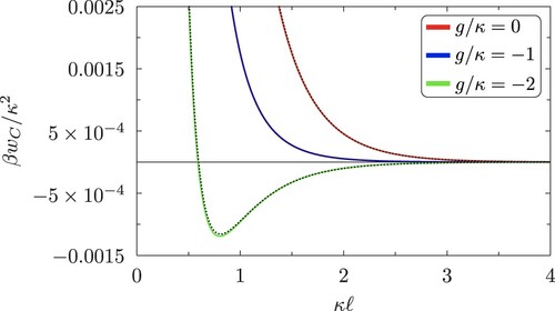
The Casimir contribution to the binding potential is qualitatively different for first-order and critical wetting transitions. This can be readily understood by focusing on its form near tri-criticality where at leading order it decays as (58) $\begin{array}{r}{w}_C\left(\ell \right)\approx \frac{{\mathrm{e}}^{-2\kappa \ell }}{32{\pi }^2\text{β}{\ell }^2}(1+2(g+\kappa \left)\ell \right)\end{array}$(58) which very accurately describes its behaviour for all film thicknesses $\kappa \ell >1$. For critical wetting ($-g>\kappa$), the Casimir term is repulsive at short distances, attractive at large distances possessing a minimum near $\ell \sim -1/(g+\kappa )$. For tri-critical and first-order wetting $w_C\left(\ell \right)$ is entirely repulsive – see Figure 2.

Figure 2. The Casimir contribution to the binding potential for a wetting layer of uniform thickness ℓ, Equation (3(3) $\begin{array}{r}{w}_C\left(\ell \right)=\frac{k_{B}T}{4\pi }{\int }_0^{\mathrm{\infty }}\mathrm{d}qq\ln (1-\frac{g+{\kappa }_q}{g-{\kappa }_q}{\mathrm{e}}^{-2{\kappa }_q\ell }),\end{array}$(3) ), illustrated for critical wetting ($g=-2\kappa$), tri-critical wetting ($g=-\kappa$) and first-order wetting (g = 0). The dashed lines are the contribution from the leading order exponential term in the expansion of $w_C\left(\ell \right)$ which is near exact over the whole range of film thicknesses.

The Casimir term strongly affects critical singularities at wetting transitions of all orders. This is most clearly apparent for tri-critical wetting ($-g=\kappa$) for which the total binding potential decays as (59) $\begin{array}{r}\frac{w\left(\ell \right)}{\gamma }=-t{\mathrm{e}}^{-\kappa \ell }+\frac{\omega }{8}\frac{{\mathrm{e}}^{-2\kappa \ell }}{(\kappa \ell {)}^2},\end{array}$(59) where $t=(T_w-T)/T_w$ is the temperature-like scaling field and $\omega =k_{B}T{\kappa }^2/4\pi \gamma$ is the dimensionless wetting parameter which controls the non-universality. Thus, it is the Casimir contribution, and not the higher-order term coming from the mean-field part, that determines the interfacial repulsion. The marginal dimension for interfacial fluctuation effects at tri-critical (and critical) wetting remains $d^{\ast }=3$ – in the sense that this is still the dimension at which capillary-wave-like interfacial fluctuations alter predictions for the film thickness, for example, based on simply minimising the binding potential $w\left(\ell \right)$ – but this does not mean that mean-field theory is correct when interfacial fluctuations are neglected as has always been thought. Mean-field is only valid if we set $d=\mathrm{\infty }$ or suppose artificially that the temperature T = 0. The Casimir contribution reveals there is a second source of thermal fluctuation effects at 3D wetting transitions in addition to interfacial wandering – something which forces us to reassess the role of thermal fluctuations and the limitations of mean-field theories of wetting. Not surprisingly the RG analysis of tri-critical wetting based on the Casimir corrected binding potential (59(59) $\begin{array}{r}\frac{w\left(\ell \right)}{\gamma }=-t{\mathrm{e}}^{-\kappa \ell }+\frac{\omega }{8}\frac{{\mathrm{e}}^{-2\kappa \ell }}{(\kappa \ell {)}^2},\end{array}$(59) ) [26] then leads to different non-universal critical exponents to those predicted previously [32].

We finish by mentioning that for critical wetting, the Casimir contribution does not alter the true critical singularities occurring in the asymptotic regime since its contribution is smaller than the two leading order exponential terms in $w_{\mathrm{M}\mathrm{F}}\left(\ell \right)$ . However, the asymptotic critical regime is negligibly small and is of no physical relevance – put colloquially, the correlation length ${\xi }_{\parallel }\propto t^{-{\nu }_{\parallel }}$ would have to be at least the size of a swimming pool in order to observe the correlation length critical exponent ${\nu }_{\parallel }\approx 3.7$ as originally predicted for the Ising model. However, the Casimir contribution strongly effects the growth of the wetting layer in the microscopic to mesoscopic range, which is the actual regime of physical relevance to simulation and experimental studies. For example, a numerical RG analysis of critical wetting with the Casimir corrected binding potential, and with the wetting parameter set at $\omega =0.8$ (which is the physical value appropriate to the Ising model and also fluids close to their critical temperature) shows that in the range $10<\kappa {\xi }_{\parallel }<1000$ the correlation length grows with an effective exponent ${\nu }_{\parallel }^{\mathrm{e}\mathrm{f}\mathrm{f}}\approx 2.0$ , as shown in Figure 3. This is the same value as that measured in the Ising model simulations [12] when the correlation length is precisely of this range. This suggests that the long controversy surrounding the nature of critical wetting transitions in three-dimensional systems with short-ranged forces may finally be coming to an end.

Figure 3. The divergence of the parallel correlation length and wetting layer thickness (inset) obtained using the numerical non-linear RG for critical wetting with $\omega =0.8$ allowing for a Casimir correction to the binding potential. The continuous dark line corresponds to the asymptotic prediction ${\xi }_{\parallel }\sim (t|\ln t{|}^{0.3}{)}^{-3.7}$ [7] which is only reached when $\kappa {\xi }_{\parallel }>{10}^{10}$ indicating that this regime is likely unobservable. The approach to this asymptotic regime is extremely broad and gradual with the growth of the correlation length for thinner films, being described by an effective exponent ${\nu }_{\parallel }^{\mathrm{e}\mathrm{f}\mathrm{f}}\approx 2$ (dashed line) very similar to that seen in Ising model simulations [12].

Acknowledgments

This paper is dedicated to the memory of three brilliant people who influenced us, and many, many others, deeply, both professionally and personally. Luis F. Rull, Kurt Binder and Michael E. Fisher.

Disclosure statement

No potential conflict of interest was reported by the author(s).

Additional information

Funding

This work was supported by Ministerio de Ciencia e Innovación (Spain) [grant number PID2021-126348NB-I00]; and Consejería de Economía, Conocimiento, Empresas y Universidad (Junta de Andalucía, Spain) [grants number US-1380729 and P20_00816], cofunded by EU FEDER. A.S. acknowledges FWF Der Wissenschaftsfonds (Austrian Science Fund) for funding through the Lise-Meitner Fellowship [grant number M 3300-N].

Appendix.

Discrete transfer matrix and continuum limit

In this Appendix, we will evaluate the partition function associated with the Hamiltonian (A1) $\begin{array}{rl}& H_n({\mathrm{\Phi }}_1,{\varphi }_1,\dots ,{\varphi }_{n-1},{\mathrm{\Phi }}_2)\\ & =\frac{{\kappa }^2ϵ{\mathrm{\Phi }}_1^2}{2}\\ & +ϵ\sum _{i=1}^n\left[\frac{1}{2{ϵ}^2}\right({\varphi }_i-{\varphi }_{i-1}{)}^2+\frac{1}{2}{\kappa }^2{\varphi }_i^2],\end{array}$(A1) with ${\varphi }_0={\mathrm{\Phi }}_1$ and ${\varphi }_n={\mathrm{\Phi }}_2$. This Hamiltonian is a discretised version of the Euclidean action H of the harmonic oscillator (A2) $\begin{array}{r}H={\int }_{{\ell }_1}^{{\ell }_2}\mathrm{d}x[\frac{1}{2}{\left(\frac{\mathrm{d}\varphi \left(x\right)}{\mathrm{d}x}\right)}^2+\frac{{\kappa }^2}{2}\varphi (x{)}^2],\end{array}$(A2) with the fields ${\varphi }_j$ being equal to $\varphi (x_j=jϵ)$. The partition function can be expressed as (A3) $\begin{array}{rl}{\mathcal{Z}}_n({\mathrm{\Phi }}_1,{\ell }_2;ϵ)& ={\left(\frac{\text{β}}{2\pi ϵ}\right)}^{(n-1)/2}{\int }_{-\mathrm{\infty }}^{\mathrm{\infty }}\mathrm{d}{\varphi }_1\cdots \\ & \times {\int }_{-\mathrm{\infty }}^{\mathrm{\infty }}\mathrm{d}{\varphi }_{n-1}{\mathrm{e}}^{-\text{β}{H}_n({\mathrm{\Phi }}_1,{\varphi }_1,\dots ,{\varphi }_{n-1},{\mathrm{\Phi }}_2)}.\end{array}$(A3) Since the exponent in the Boltzmann factor is a quadratic form in the fields ${\varphi }_i$, it is convenient to assemble the fields into a vector ${\mathit{\varphi }}^{†}=({\varphi }_1,\dots ,{\varphi }_{n-1})$ and then the discretised Hamiltonian $H_n$ can be expressed as (A4) $\begin{array}{rl}{H}_n& =\frac{1}{2ϵ}{\mathit{\varphi }}^{†}\cdot {\mathsf{C}}_{\mathsf{n}}\cdot \mathit{\varphi }\mathsf{+}\frac{\mathsf{(}\mathsf{1}\mathsf{+}{\kappa }^{\mathsf{2}}{ϵ}^{\mathsf{2}}\mathsf{)}}{\mathsf{2}ϵ}\mathsf{(}{\mathsf{\Phi }}_{\mathsf{1}}^{\mathsf{2}}\mathsf{+}{\mathsf{\Phi }}_{\mathsf{2}}^{\mathsf{2}}\mathsf{)}\\ & -\frac{{\mathrm{\Phi }}_1{\varphi }_1+{\mathrm{\Phi }}_2{\varphi }_{n-1}}{ϵ},\end{array}$(A4) where ${\mathsf{\text{C}}}_n$ is a $(n-1)\times (n-1)$ matrix whose entries are given by the Hessian of the quadratic form associated to $H_n$; thus, (A5) $\begin{array}{r}{\left({\mathsf{C}}_{\mathsf{n}}\right)}_{i,j}=\frac{1}{2}\frac{{\mathrm{\partial }}^2}{\mathrm{\partial }{\varphi }_i\mathrm{\partial }{\varphi }_j}({\mathit{\varphi }}^{†}\cdot {\mathsf{C}}_{\mathsf{n}}\cdot \mathit{\varphi }).\end{array}$(A5) The matrix ${\mathsf{\text{C}}}_n$ has the tridiagonal structure shown in (A6(A6) $\begin{array}{r}{\mathsf{C}}_{\mathsf{n}}\mathsf{=}\left(\begin{array}{cccccc}2p& -1& 0& \dots & & 0\\ -1& 2p& -1& & & ⋮\\ 0& -1& \ddots & \ddots & & \\ ⋮& & \ddots & & & 0\\ & & & & & -1\\ 0& \dots & & 0& -1& 2p\end{array}\right)\mathsf{,}\end{array}$(A6) ) (A6) $\begin{array}{r}{\mathsf{C}}_{\mathsf{n}}\mathsf{=}\left(\begin{array}{cccccc}2p& -1& 0& \dots & & 0\\ -1& 2p& -1& & & ⋮\\ 0& -1& \ddots & \ddots & & \\ ⋮& & \ddots & & & 0\\ & & & & & -1\\ 0& \dots & & 0& -1& 2p\end{array}\right)\mathsf{,}\end{array}$(A6) with $p=1+{\kappa }^2{ϵ}^2/2$. Let us define the mean-field fields ${\varphi }_i^{\mathrm{M}\mathrm{F}}$ as the solution of the following equations: (A7) $\begin{array}{rl}{\varphi }_0^{\mathrm{M}\mathrm{F}}& ={\mathrm{\Phi }}_1,{\varphi }_n^{\mathrm{M}\mathrm{F}}={\mathrm{\Phi }}_2,\\ & -{\varphi }_{i-1}^{\mathrm{M}\mathrm{F}}+2p{\varphi }_i^{\mathrm{M}\mathrm{F}}-{\varphi }_{i+1}^{\mathrm{M}\mathrm{F}}=0,i=1,\dots ,n-1.\end{array}$(A7) The latter recursion relationship for $i=2,\dots ,n-2$ has as general solution (A8) $\begin{array}{r}{\varphi }_i^{\mathrm{M}\mathrm{F}}=A{\lambda }_{+}^i+B{\lambda }_{-}^i,\end{array}$(A8) where ${\lambda }_{\pm }=p\pm \sqrt{p^2-1}$ are the roots of the characteristic equation (A9) $\begin{array}{r}{\lambda }^2-2p\lambda +1=0.\end{array}$(A9) We can fix A and B by imposing the conditions $2p{\varphi }_1^{\mathrm{M}\mathrm{F}}-{\varphi }_2^{\mathrm{M}\mathrm{F}}={\mathrm{\Phi }}_1$ and $2{\varphi }_{n-1}^{\mathrm{M}\mathrm{F}}-{\varphi }_{n-2}^{\mathrm{M}\mathrm{F}}={\mathrm{\Phi }}_2$ ; hence, it follows that (A10) $\begin{array}{r}{\varphi }_i^{\mathrm{M}\mathrm{F}}={\mathrm{\Phi }}_1\frac{{\lambda }_{+}^{n-i}-{\lambda }_{-}^{n-i}}{{\lambda }_{+}^n-{\lambda }_{-}^n}+{\mathrm{\Phi }}_2\frac{{\lambda }_{+}^i-{\lambda }_{-}^i}{{\lambda }_{+}^n-{\lambda }_{-}^n}.\end{array}$(A10) By using the property ${\lambda }_{+}{\lambda }_{-}=1$, we have (A11) $\begin{array}{r}{\varphi }_i^{\mathrm{M}\mathrm{F}}={\mathrm{\Phi }}_1\frac{\sinh \left[\right(n-i){\cosh }^{-1}(p\left)\right]}{\sinh (n{\cosh }^{-1}(p\left)\right)}+{\mathrm{\Phi }}_2\frac{\sinh [i{\cosh }^{-1}(p\left)\right]}{\sinh (n{\cosh }^{-1}(p\left)\right)}.\end{array}$(A11) If we write ${\varphi }_i={\varphi }_i^{\mathrm{M}\mathrm{F}}+{\psi }_i$ for $i=0,\dots ,n$, then the discrete Hamiltonian can be expressed as (A12) $\begin{array}{rl}{H}_n({\mathrm{\Phi }}_1,{\varphi }_1,\dots ,{\varphi }_{n-1},{\mathrm{\Phi }}_2)& =H_n({\mathrm{\Phi }}_1,{\varphi }_1^{\mathrm{M}\mathrm{F}},\dots ,{\varphi }_{n-1}^{\mathrm{M}\mathrm{F}},{\mathrm{\Phi }}_2)\\ & +H_n(0,{\psi }_1,\dots ,{\psi }_{n-1},0),\end{array}$(A12) and, consequently, Equation (A3(A3) $\begin{array}{rl}{\mathcal{Z}}_n({\mathrm{\Phi }}_1,{\ell }_2;ϵ)& ={\left(\frac{\text{β}}{2\pi ϵ}\right)}^{(n-1)/2}{\int }_{-\mathrm{\infty }}^{\mathrm{\infty }}\mathrm{d}{\varphi }_1\cdots \\ & \times {\int }_{-\mathrm{\infty }}^{\mathrm{\infty }}\mathrm{d}{\varphi }_{n-1}{\mathrm{e}}^{-\text{β}{H}_n({\mathrm{\Phi }}_1,{\varphi }_1,\dots ,{\varphi }_{n-1},{\mathrm{\Phi }}_2)}.\end{array}$(A3) ) reads (A13) $\begin{array}{r}{\mathcal{Z}}_n({\mathrm{\Phi }}_1,{\mathrm{\Phi }}_2;ϵ)={\mathcal{Z}}_n(0,0;ϵ){\mathrm{e}}^{-\text{β}{H}_n({\mathrm{\Phi }}_1,{\varphi }_1^{\mathrm{M}\mathrm{F}},\dots ,{\varphi }_{n-1}^{\mathrm{M}\mathrm{F}},{\mathrm{\Phi }}_2)},\end{array}$(A13) where, after substituting Equation (A22(A22) $\begin{array}{r}s-lim{\varphi }_i^{\mathrm{M}\mathrm{F}}={\mathrm{\Phi }}_1\frac{\sinh \kappa ({\ell }_{21}-x)}{\sinh \kappa {\ell }_{21}}+{\mathrm{\Phi }}_2\frac{\sinh \kappa x}{\sinh \kappa {\ell }_{21}},\end{array}$(A22) ) into Equation (A4(A4) $\begin{array}{rl}{H}_n& =\frac{1}{2ϵ}{\mathit{\varphi }}^{†}\cdot {\mathsf{C}}_{\mathsf{n}}\cdot \mathit{\varphi }\mathsf{+}\frac{\mathsf{(}\mathsf{1}\mathsf{+}{\kappa }^{\mathsf{2}}{ϵ}^{\mathsf{2}}\mathsf{)}}{\mathsf{2}ϵ}\mathsf{(}{\mathsf{\Phi }}_{\mathsf{1}}^{\mathsf{2}}\mathsf{+}{\mathsf{\Phi }}_{\mathsf{2}}^{\mathsf{2}}\mathsf{)}\\ & -\frac{{\mathrm{\Phi }}_1{\varphi }_1+{\mathrm{\Phi }}_2{\varphi }_{n-1}}{ϵ},\end{array}$(A4) ) and after some algebra, we get that (A14) $\begin{array}{rl}& H_n({\mathrm{\Phi }}_1,{\varphi }_1^{\mathrm{M}\mathrm{F}},\dots ,{\varphi }_{n-1}^{\mathrm{M}\mathrm{F}},{\mathrm{\Phi }}_2)=-\frac{{\mathrm{\Phi }}_1{\mathrm{\Phi }}_2}{ϵ}\frac{\sinh ({\cosh }^{-1}(p)}{\sinh (n{\cosh }^{-1}(p\left)\right)}\\ & +\frac{{\mathrm{\Phi }}_1^2+{\mathrm{\Phi }}_2^2}{2ϵ}(p-1+\coth (n{\cosh }^{-1}\left(p\right))\sinh ({\cosh }^{-1}\left(p\right)\left)\right).\end{array}$(A14) The partition function ${\mathcal{Z}}_n(0,0,ϵ)$ can be evaluated as the following Gaussian integral: (A15) $\begin{array}{rl}{\mathcal{Z}}_n(0,0;ϵ)& ={\left(\frac{\text{β}}{2\pi ϵ}\right)}^{(n-1)/2}{\int }_{-\mathrm{\infty }}^{\mathrm{\infty }}\mathrm{d}{\psi }_1\\ & \cdots {\int }_{-\mathrm{\infty }}^{\mathrm{\infty }}\mathrm{d}{\psi }_{n-1}{\mathrm{e}}^{-\frac{\text{β}}{2ϵ}{\mathit{\psi }}^{†}\cdot {\mathsf{C}}_{\mathsf{n}}\cdot \mathit{\psi }}=\sqrt{\frac{1}{d_n}},\end{array}$(A15) where $d_n\equiv det{\mathsf{\text{C}}}_n$. In order to compute the determinant, we first note that it satisfies the recursion relation (A16) $\begin{array}{r}{d}_n=(2+{\kappa }^2{ϵ}^2)d_{n-1}-d_{n-2},\end{array}$(A16) similar to Equation (A7(A7) $\begin{array}{rl}{\varphi }_0^{\mathrm{M}\mathrm{F}}& ={\mathrm{\Phi }}_1,{\varphi }_n^{\mathrm{M}\mathrm{F}}={\mathrm{\Phi }}_2,\\ & -{\varphi }_{i-1}^{\mathrm{M}\mathrm{F}}+2p{\varphi }_i^{\mathrm{M}\mathrm{F}}-{\varphi }_{i+1}^{\mathrm{M}\mathrm{F}}=0,i=1,\dots ,n-1.\end{array}$(A7) ), so its solution can be written as (A17) $\begin{array}{r}{d}_n=A{\lambda }_{+}^{n-1}+B{\lambda }_{-}^{n-1},\end{array}$(A17) From the initial conditions $d_1=1$ and $d_2=2+{\kappa }^2{ϵ}^2,$ we can fix A and B; hence, it follows that (A18) $\begin{array}{r}{d}_n=\frac{{\lambda }_{+}^n-{\lambda }_{-}^n}{{\lambda }_{+}-{\lambda }_{-}}.\end{array}$(A18) By using the property ${\lambda }_{+}{\lambda }_{-}=1$, we have (A19) $\begin{array}{r}{d}_n=\frac{\sinh [n{\cosh }^{-1}(p\left)\right]}{\sinh ({\cosh }^{-1}(p\left)\right)}=\frac{\sinh [n{\cosh }^{-1}(p\left)\right]}{\sqrt{p^2-1}}.\end{array}$(A19) These solutions are related to the path-integral continuous formulation, since (A20) $\begin{array}{r}\mathcal{Z}({\mathrm{\Phi }}_1,{\ell }_1|{\mathrm{\Phi }}_2,{\ell }_2)=\int \mathcal{D}\varphi {\mathrm{e}}^{-\text{β}H},\end{array}$(A20) where the path integral is over all the continuous paths $\varphi \left(x\right)$ on $[{\ell }_1,{\ell }_2]$ such that $\varphi \left({\ell }_1\right)={\mathrm{\Phi }}_1$ and $\varphi \left({\ell }_2\right)={\mathrm{\Phi }}_2$. This can be obtained as the following scaling limit (denoted as $s-lim$) in which $n\to \mathrm{\infty }$, $ϵ\to 0$, with finite ${\ell }_2-{\ell }_1=nϵ$ [33] (A21) $\begin{array}{r}\mathcal{Z}({\mathrm{\Phi }}_1,{\ell }_1|{\mathrm{\Phi }}_2,{\ell }_2)=s-lim\left[\sqrt{\frac{\text{β}}{2\pi ϵ}}{\mathcal{Z}}_n\right({\mathrm{\Phi }}_1,{\mathrm{\Phi }}_2;ϵ\left)\right].\end{array}$(A21)

First, we perform the scaling limit of the above results. Thus Equation (A22(A22) $\begin{array}{r}s-lim{\varphi }_i^{\mathrm{M}\mathrm{F}}={\mathrm{\Phi }}_1\frac{\sinh \kappa ({\ell }_{21}-x)}{\sinh \kappa {\ell }_{21}}+{\mathrm{\Phi }}_2\frac{\sinh \kappa x}{\sinh \kappa {\ell }_{21}},\end{array}$(A22) ) leads to, writing ${\ell }_{21}={\ell }_2-{\ell }_1$ (A22) $\begin{array}{r}s-lim{\varphi }_i^{\mathrm{M}\mathrm{F}}={\mathrm{\Phi }}_1\frac{\sinh \kappa ({\ell }_{21}-x)}{\sinh \kappa {\ell }_{21}}+{\mathrm{\Phi }}_2\frac{\sinh \kappa x}{\sinh \kappa {\ell }_{21}},\end{array}$(A22) which is the solution of the mean-field equation $d^2{\varphi }^{\mathrm{M}\mathrm{F}}/\mathrm{d}{x}^2-{\kappa }^2{\varphi }^{\mathrm{M}\mathrm{F}}=0$ subject to the boundary conditions ${\varphi }^{\mathrm{M}\mathrm{F}}\left({\ell }_1\right)={\mathrm{\Phi }}_1$ and ${\varphi }^{\mathrm{M}\mathrm{F}}\left({\ell }_2\right)={\mathrm{\Phi }}_2$ (i.e. the scaling limit of the Equation (A7(A7) $\begin{array}{rl}{\varphi }_0^{\mathrm{M}\mathrm{F}}& ={\mathrm{\Phi }}_1,{\varphi }_n^{\mathrm{M}\mathrm{F}}={\mathrm{\Phi }}_2,\\ & -{\varphi }_{i-1}^{\mathrm{M}\mathrm{F}}+2p{\varphi }_i^{\mathrm{M}\mathrm{F}}-{\varphi }_{i+1}^{\mathrm{M}\mathrm{F}}=0,i=1,\dots ,n-1.\end{array}$(A7) )). The mean-field energy, on the other hand, can be obtained from Equation (A14(A14) $\begin{array}{rl}& H_n({\mathrm{\Phi }}_1,{\varphi }_1^{\mathrm{M}\mathrm{F}},\dots ,{\varphi }_{n-1}^{\mathrm{M}\mathrm{F}},{\mathrm{\Phi }}_2)=-\frac{{\mathrm{\Phi }}_1{\mathrm{\Phi }}_2}{ϵ}\frac{\sinh ({\cosh }^{-1}(p)}{\sinh (n{\cosh }^{-1}(p\left)\right)}\\ & +\frac{{\mathrm{\Phi }}_1^2+{\mathrm{\Phi }}_2^2}{2ϵ}(p-1+\coth (n{\cosh }^{-1}\left(p\right))\sinh ({\cosh }^{-1}\left(p\right)\left)\right).\end{array}$(A14) ) as (A23) $\begin{array}{rl}& s-lim{H}_n({\mathrm{\Phi }}_1,{\varphi }_1^{\mathrm{M}\mathrm{F}},\dots ,{\varphi }_{n-1}^{\mathrm{M}\mathrm{F}},{\mathrm{\Phi }}_2)\\ & =-\frac{\kappa {\mathrm{\Phi }}_1{\mathrm{\Phi }}_2}{\sinh \kappa {\ell }_{21}}+\frac{\kappa ({\mathrm{\Phi }}_1^2+{\mathrm{\Phi }}_2^2)}{2}\coth \left(\kappa {\ell }_{21}\right).\end{array}$(A23) Finally, (A24) $\begin{array}{r}s-lim\left(ϵd_n\right)=\frac{\sinh \kappa {\ell }_{21}}{\kappa }.\end{array}$(A24) Therefore, Equation (A21(A21) $\begin{array}{r}\mathcal{Z}({\mathrm{\Phi }}_1,{\ell }_1|{\mathrm{\Phi }}_2,{\ell }_2)=s-lim\left[\sqrt{\frac{\text{β}}{2\pi ϵ}}{\mathcal{Z}}_n\right({\mathrm{\Phi }}_1,{\mathrm{\Phi }}_2;ϵ\left)\right].\end{array}$(A21) ) indeed leads to Equation (26(26) $\begin{array}{rl}& \mathcal{Z}({\varphi }_1,{\ell }_1|{\varphi }_2,{\ell }_2)\\ & =\sqrt{\frac{\text{β}\kappa }{2\pi \sinh \kappa {\ell }_{21}}}\\ & \times \exp (\frac{\text{β}\kappa {\varphi }_1{\varphi }_2}{\sinh \kappa {\ell }_{21}}-\frac{\text{β}\kappa ({\varphi }_1^2+{\varphi }_2^2)}{2}\coth \kappa {\ell }_{21}),\end{array}$(26) ), which was obtained directly in Section 3, within the continuum LGW model description, using the path integral formalism.

References

- S. Dietrich, in Phase Transitions and Critical Phenomena, edited by C. Domb and J.L. Lebowitz (Academic, London, 1988), Vol. 12, p. 1.
- M. Schick, in Liquids at Interfaces, edited by J. Chavrolin, J.-F. Joanny and J. Zinn-Justin (Elsevier, Amsterdam, 1990), p. 415.
- G. Forgacs, R. Lipowsky and T.M. Nieuwenhuizen, in Phase Transitions and Critical Phenomena, edited by C. Domb and J. L. Lebowitz (Academic Press, London, 1991), Vol. 14, Chap. 2.
- D. Bonn, J. Eggers, J. Indekeu, J. Meunier and E. Rolley, Rev. Mod. Phys. 81 (2), 739 (2009). doi:10.1103/RevModPhys.81.739
- R. Lipowsky, D.M. Kroll and R.K.P. Zia, Phys. Rev. B 27 (7), 4499 (1983). doi:10.1103/PhysRevB.27.4499
- E. Brézin, B.I. Halperin and S. Leibler, Phys. Rev. Lett. 50 (18), 1387 (1983). doi:10.1103/PhysRevLett.50.1387
- D.S. Fisher and D.A. Huse, Phys. Rev. B 32 (1), 247 (1985). doi:10.1103/PhysRevB.32.247
- K. Binder, D.P. Landau and D.M. Kroll, Phys. Rev. Lett. 56 (21), 2272 (1986). doi:10.1103/PhysRevLett.56.2272
- K. Binder and D.P. Landau, Phys. Rev. B 37 (4), 1745 (1988). doi:10.1103/PhysRevB.37.1745
- A.O. Parry, R. Evans and K. Binder, Phys. Rev. B 43 (13), 11535 (1991). doi:10.1103/PhysRevB.43.11535
- K. Binder, D.P. Landau and S. Wansleben, Phys. Rev. B 40 (10), 6971 (1989). doi:10.1103/PhysRevB.40.6971
- P. Bryk and K. Binder, Phys. Rev. E 88 (3), 030401 (2013). doi:10.1103/PhysRevE.88.030401
- P. Bryk and A.P. Terzyk, Materials 14 (23), 7138 (2021). doi:10.3390/ma14237138
- R. Evans, D.C. Hoyle and A.O. Parry, Phys. Rev. A 45 (6), 3823 (1992). doi:10.1103/PhysRevA.45.3823
- M.E. Fisher and H. Wen, Phys. Rev. Lett. 68 (24), 3654 (1992). doi:10.1103/PhysRevLett.68.3654
- H. Nakanishi and M.E. Fisher, Phys. Rev. Lett. 49 (21), 1565 (1982). doi:10.1103/PhysRevLett.49.1565
- M.E. Fisher and A.J. Jin, Phys. Rev. Lett. 69 (5), 792 (1992). doi:10.1103/PhysRevLett.69.792
- A.J. Jin and M.E. Fisher, Phys. Rev. B 48 (4), 2642 (1993). doi:10.1103/PhysRevB.48.2642
- M.E. Fisher, A.J. Jin and A.O. Parry, Bunsenges. Phys. Chem. 98 (3), 357 (1994). doi:10.1002/bbpc.19940980314
- A.O. Parry, J.M. Romero-Enrique and A. Lazarides, Phys. Rev. Lett. 93 (8), 086104 (2004). doi:10.1103/PhysRevLett.93.086104
- A.O. Parry, C. Rascón, N.R. Bernardino and J.M. Romero-Enrique, J. Phys.: Condens. Matter 20 (49), 494234 (2008). doi:10.1088/0953-8984/20/49/494234
- A.O. Parry, C. Rascón, N.R. Bernardino and J.M. Romero-Enrique, J. Phys.: Condens. Matter 18 (28), 6433 (2006). doi:10.1088/0953-8984/18/28/001
- J.M. Romero-Enrique, A. Squarcini, A.O. Parry and P.M. Goldbart, Phys. Rev. E 97 (6), 062804 (2018). doi:10.1103/PhysRevE.97.062804
- R. Lipowsky and M.E. Fisher, Phys. Rev. B 36 (4), 2126 (1987). doi:10.1103/PhysRevB.36.2126
- S. Dietrich and M. Napiórkowski, Phys. Rev. A 43 (4), 1861 (1991). doi:10.1103/PhysRevA.43.1861
- A. Squarcini, J.M. Romero-Enrique and A.O. Parry, Phys. Rev. Lett. 128 (19), 195701 (2022). doi:10.1103/PhysRevLett.128.195701
- M. Vallade and J. Lajzerowicz, J. Phys. 42 (11), 1505 (1981). doi:10.1051/jphys:0198100420110150500
- T.W. Burkhardt, Phys. Rev. B 40 (10), 6987 (1989). doi:10.1103/PhysRevB.40.6987
- A. Adjari, B. Duplantier, D. Hone, L. Peliti and J. Prost, J. Phys. II France 2, 487 (1992). doi:10.1051/jp2:1992145
- M.E. Fisher and A.J. Jin, Phys. Rev. B 44 (3), 1430 (1991). doi:10.1103/PhysRevB.44.1430
- B. Kastening and V. Dohm, Phys. Rev. E 81 (6), 061106 (2010). doi:10.1103/PhysRevE.81.061106
- C.J. Boulter and F. Clarysse, EPJE 5, 465 (2001). doi:10.1007/s101890170053
- R.P. Feynman and A.R. Hibbs, Quantum Mechanics and Path Integrals (McGraw-Hill, New York, 1965).