High-precision Ramsey-comb spectroscopy on molecular deuterium for tests of molecular quantum theory

Abstract

Precision spectroscopy of simple, calculable molecules has become an important tool to compare experiments with theory in an effort to test our understanding of the fundamental laws of physics. For this purpose, we have measured the $\mathrm{E}\mathrm{F}{}^1{\mathrm{\Sigma }}_g^{+}(v^{\prime }=0,N^{\prime }=0)\leftarrow \mathrm{X}{}^1{\mathrm{\Sigma }}_g^{+}(v^{″}=0,N^{″}=0)$  transition frequency of molecular deuterium (${\mathrm{D}}_2$) with unprecedented accuracy. We use Ramsey-Comb spectroscopy at deep-ultraviolet wavelengths (201 nm) with a two-photon, Doppler-free interrogation scheme. The resulting transition frequency is $f=2,981,779,227,578\left(19\right)$ kHz. The 1-σ uncertainty of 19 kHz represents an improvement of more than two orders of magnitude compared to the best previous measurement. In this paper, we give an extensive description of our methods and the experimental apparatus that we employed. Particular attention is given to aspects that we recently improved, such as the frequency comb laser system, the method of signal recording, and the cryogenic ${\mathrm{D}}_2$ molecular beam apparatus. In combination with future measurements of the ionisation energy of the EF state, our measurement paves the way for an improved determination of the ground state ionisation and dissociation energy of molecular deuterium.

Keywords:

• High-precision spectroscopy
• Ramsey-comb spectroscopy
• deuterium
• dissociation energy
• ionisation energy

View correction statement:

Correction

1. Introduction

Comparing experimentally measured transition frequencies in atoms and molecules with those obtained from theory calculations is a powerful method to test our understanding of the fundamental laws of physics. However, calculations of the energy levels does require accurate values of the fundamental constants. By measuring different transitions within one system, and by measuring in different systems, it is possible to disentangle the laws of physics from the constants and determine both. For many decades, atomic hydrogen has been a cornerstone for such spectroscopic tests [1,2], and it enables a very accurate determination of the Rydberg constant and the proton charge radius. Surprisingly, spectroscopic measurements in muonic hydrogen (with a bound muon instead of an electron) led to a substantially different proton radius and Rydberg constant [3,4]. New measurements in normal (electronic) hydrogen now tend to confirm the smaller proton radius from the muonic results [5,6], but not all of them [7,8]. Moreover, a significant 7σ discrepancy still exists for the deuteron charge radius (although no new measurements have been published) [9]. This history has made clear that measurements need to be done in different systems. Molecules are very interesting in that respect because they have extra degrees of freedom (vibration and rotation) that enable tests of a different nature and of different fundamental constants. An example is the recent determination of the proton to electron mass ratio from spectroscopy of HD${}^{+}$ ions [10,11].

Another interesting system is the simplest neutral molecule, ${\mathrm{H}}_2$. With two interacting electrons, the calculations for ${\mathrm{H}}_2$ are much harder than for HD${}^{+}$ or H. For more than a 100 years, the dissociation energy of molecular hydrogen, $D_0\left({\mathrm{H}}_2\right)$, has stood as a benchmark value for a comparison between theory and experiment, as it can be calculated best. In the past 10 years great progress has been made, both experimentally (see e.g. [12,13]) and theoretically [14,15]. At present there is an agreement between experiment and theory within 1 MHz on the value of $D_0\left({\mathrm{H}}_2\right)$, and on its counterpart in molecular deuterium, $D_0\left({\mathrm{D}}_2\right)$ [12,16,17]. Interestingly, rovibrational transition energies measured in the ground state of HD systematically deviate from theory by 1.9 MHz [18]. These spectroscopic measurements currently test the accuracy of molecular quantum mechanical calculations.

In principle, values of fundamental constants can also be investigated. The proton charge radius, in particular, is an important parameter for the calculation of the dissociation energy of molecular hydrogen and can be probed by comparing theory and experiments. However, current experimental and theoretical results are not yet sufficiently accurate to test its influence in ${\mathrm{H}}_2$; an accuracy better than 10 kHz on the value of $D_0\left({\mathrm{H}}_2\right)$ is required to measure the charge radius of the proton at the 1% level. The situation is better in molecular deuterium as the nuclear size effect is 7 times bigger than in ${\mathrm{H}}_2$, which amounts to a contribution of about 6.1 MHz to the total value of the dissociation energy $D_0\left({\mathrm{D}}_2\right)$. With recent measurements via the GK state, the experimental determination of $D_0\left({\mathrm{D}}_2\right)$ has been improved considerably, reaching an accuracy of 780 kHz [13,19]. The obtained $D_0\left({\mathrm{D}}_2\right)$ value agrees very well with its most precise theoretical determination [16], also with an accuracy of 780 kHz.

The subject of this paper is a new measurement of the $\mathrm{E}\mathrm{F}{}^1{\mathrm{\Sigma }}_g^{+}(v^{\prime }=0,N^{\prime }=0)\leftarrow \mathrm{X}{}^1{\mathrm{\Sigma }}_g^{+}(v^{″}=0,N^{″}=0)$ transition¹ in ${\mathrm{D}}_2$. This will enable an improved determination of $D_0\left({\mathrm{D}}_2\right)$ via the EF state, once also the accuracy of the ionzation energy of the EF state is improved. It will then allow for a new generation of tests of molecular structure calculations and enable a meaningful test of the deuteron finite nuclear-size effect in a neutral molecule.

The most accurate method to determine $D_0\left({\mathrm{D}}_2\right)$ is through the successful approach established for ${\mathrm{H}}_2$ [19,20], by combining three different energy intervals as shown in Figure 1. The so-called thermodynamic cycle can be written as: (1) $D_0\left({\mathrm{D}}_2\right)=E_{\mathrm{I}}\left({\mathrm{D}}_2\right)+D_0\left({\mathrm{D}}_2^{+}\right)-E_{\mathrm{I}}\left(\mathrm{D}\right),$(1) where $E_I($D₂$)$ is the ionisation energy of molecular deuterium, $D_0\left({\mathrm{D}}_2^{+}\right)$ is the dissociation energy of the molecular deuterium ion, and $E_I\left(D\right)$ is the ionisation energy of the deuterium atom. Because $D_0\left({\mathrm{D}}_2^{+}\right)+E_{\mathrm{I}}\left(\mathrm{D}\right)=E_{\mathrm{I}}\left({\mathrm{D}}_2^{+}\right)$, we can write: (2) $D_0\left({\mathrm{D}}_2\right)=E_{\mathrm{I}}\left({\mathrm{D}}_2\right)+E_{\mathrm{I}}\left({\mathrm{D}}_2^{+}\right)-2E_{\mathrm{I}}\left(\mathrm{D}\right),$(2) As is the case in ${\mathrm{H}}_2$, the determination of the ionisation energy $E_{\mathrm{I}}($D₂$)$ is currently more than one order of magnitude less accurate than the two other terms–see Table 1. Therefore the experimental uncertainty of $E_{\mathrm{I}}($D₂$)$ needs to be improved to obtain a more accurate determination of the dissociation energy $D_0\left({\mathrm{D}}_2\right)$. Experimentally, $E_{\mathrm{I}}($D₂$)$ is determined in two major parts [13,19–21]. First by measuring the two-photon transition from the electronic ground state of molecular deuterium to the electronically-excited EF or GK state (performed in Amsterdam). This is then combined with the second part, consisting of a determination of the ionisation energy of the EF or GK electronic state (in Zürich) by laser excitation to a Rydberg state, followed by millimetre-wave (mmW) spectroscopy and multi-channel quantum defect (MQDT) theory to extrapolate to the ionisation threshold–see Figure 1 for the scheme via the EF state.

Figure 1. The dissociation energy of ${\mathrm{D}}_2$ can be determined with high accuracy by combining the ionisation energy of ${\mathrm{D}}_2$ and D with the dissociation energy of ${\mathrm{D}}_2^{+}$ (see Equations (1(1) $D_0\left({\mathrm{D}}_2\right)=E_{\mathrm{I}}\left({\mathrm{D}}_2\right)+D_0\left({\mathrm{D}}_2^{+}\right)-E_{\mathrm{I}}\left(\mathrm{D}\right),$(1) ) and 2(2) $D_0\left({\mathrm{D}}_2\right)=E_{\mathrm{I}}\left({\mathrm{D}}_2\right)+E_{\mathrm{I}}\left({\mathrm{D}}_2^{+}\right)-2E_{\mathrm{I}}\left(\mathrm{D}\right),$(2) ). The ionisation energy of ${\mathrm{D}}_2$ is currently the source of the highest uncertainty in the evaluation of its dissociation energy. What is measured in this study is the $\mathrm{E}\mathrm{F}{}^1{\mathrm{\Sigma }}_g^{+}(v^{\prime }=0,N^{\prime }=0)\leftarrow \mathrm{X}{}^1{\mathrm{\Sigma }}_g^{+}(v^{″}=0,N^{″}=0)$  transition, indicated with Q${}_0$. The ${\mathrm{D}}_2$ ionisation energy for ortho-${\mathrm{D}}_2$ with $N^{″}$=0 (or para-${\mathrm{D}}_2$ with $N^{″}$=1) is obtained by combining several experimentally-determined transition energies starting from the electronic and vibrational ground state, as shown on the right.

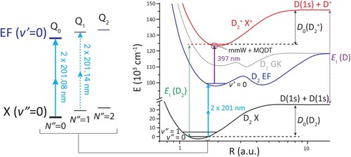
Table 1. Overview of the best previously determined dissociation energy (experiment and theory) and ionisation energy of ${\mathrm{D}}_2$, measured via the GK state, with the energy intervals required for the determination.

	Energy level interval	Value (cm${}^{-1}$)	Uncertainty (kHz)	Reference
(1)	$E_{\mathrm{I}}^{N=0}$(${\mathrm{D}}_2$)${}^{\mathrm{a}}=\left(4\right)-\left(5\right)+\left(6\right)$	124,745.393739(26)	780	[13]
(2)	$D_0^{N=0}$(${\mathrm{D}}_2$)${}^{\mathrm{a}}$ through GK	36,748.362282(26)	780	[13]
(3)	$D_0^{N=0}$(${\mathrm{D}}_2$)${}^{\mathrm{b}}$	36,748.362342(26)	780	[16]
(4)	$\mathrm{G}\mathrm{K}(v^{\prime }=1,N^{\prime }=2)\leftarrow \mathrm{X}(v^{″}=0,N^{″}=0)$ (${\mathrm{D}}_2$)${}^{\mathrm{a}}$	112,099.087712(15)	450	[13]
(5)	$\mathrm{G}\mathrm{K}(v^{\prime }=1,N^{\prime }=2)\leftarrow \mathrm{G}\mathrm{K}(v^{″}=0,N^{″}=2)$ (${\mathrm{D}}_2$)${}^{\mathrm{a}}$	333.038775(7)	210	[13]
(6)	${\mathrm{X}}^{+}(v^{+}=0,N^{+}=0)\leftarrow \mathrm{G}\mathrm{K}(v^{″}=0,N^{″}=2)$ (${\mathrm{D}}_2$)${}^{\mathrm{a}}$	12,979.344802(20)	600	[13]
(7)	$E_{\mathrm{I}}^{N=0}$(D)${}^{\mathrm{b}}$	109,708.61455294(17)	5	[22]
(8)	$E_{\mathrm{I}}^{N=0}$(${\mathrm{D}}_2^{+}$)${}^{\mathrm{b}}$	131,420.1976492(8)	24	[23]
(9)	$D_0^{N=1}$(${\mathrm{H}}_2$)${}^{\mathrm{a}}$ through EF	35,999.582834(11)	340	[12]
(10)	$D_0^{N=1}$(${\mathrm{H}}_2$)${}^{\mathrm{b}}$	35,999.582820(26)	780	[14]
(11)	$D_0^{N=0}$(${\mathrm{H}}_2$)${}^{\mathrm{c}}$ through GK	36,118.069605(31)	940	[17]
(12)	$D_0^{N=0}$(${\mathrm{H}}_2$)${}^{\mathrm{b}}$	36,118.069632(26)	780	[14]

Notes: In this table N indicates the rotational quantum number. The last part of the table also lists the most recent determinations of the dissociation energy for ortho- (N = 1) and para-${\mathrm{H}}_2$ (N = 0), measured through the EF and GK state respectively.

${}^{\mathrm{a}}$ experiment

${}^{\mathrm{b}}$ theory

${}^{\mathrm{c}}$ combination of theory and experiment

In this work, we improve the previous most accurate determination of the $\mathrm{E}\mathrm{F}{}^1{\mathrm{\Sigma }}_g^{+}(v^{\prime }=0,N^{\prime }=0)\leftarrow \mathrm{X}{}^1{\mathrm{\Sigma }}_g^{+}(v^{″}=0,N^{″}=0)$  transition frequency of ${\mathrm{D}}_2$ [24] by more than two orders of magnitude, reaching an accuracy of 19 kHz. This is made possible by the roughly 4 times longer lifetime of the EF state compared to the GK, and the use of the Ramsey-comb spectroscopy method. In combination with the upcoming measurements of the EF state ionisation energy by the group at the ETH Zürich, this will allow for a much-improved determination of the $E_I($D₂$)$ ionisation energy via the EF state.

In the following sections, we give a detailed description of the experimental setup and measurement methods we used. The paper is organised as follows: in Section 2, we describe the Ramsey-comb spectroscopy technique that was developed in our lab to perform high-precision spectroscopy of atomic and molecular systems [25,26]. In Section 3, we describe the Ramsey-comb laser system that produces high-energy and phase-coherent NIR laser pulses at a central wavelength of 804.32 nm, followed by a description of the upconversion to the deep ultraviolet (DUV) at 201.08 nm. We also describe the production of a cold and slow beam of ${\mathrm{D}}_2$ molecules and discuss the two-photon, Doppler-free laser excitation at 201.08 nm, and the detection scheme that we implemented. In Section 4 we present the data-taking and data-analysis methods that we used to extract the transition frequency, including a thorough evaluation of the systematic effects contributing to the error budget.

2. The Ramsey-comb spectroscopy principle

Ramsey-comb spectroscopy is a technique invented in our group for precision spectroscopy of atomic and molecular systems, based on two intense, phase-coherent ultrashort laser pulses. The principle has a resemblance to Ramsey spectroscopy [27,28], but instead of RF pulses, 2 amplified pulses from a frequency comb laser are used [25,26]. The frequency comb laser is used as a source of well-controlled and phase-coherent pulses. The amplification of only 2 pulses from the full pulse train of the comb enables pulse energies of several mJ, which greatly simplifies nonlinear upconversion to shorter wavelengths for spectroscopy in the DUV [21,29], as required in the current study, or shorter wavelengths through high-harmonic generation (HHG) [30,31].

In the following, we assume (realistically) that the excitation probability of ${\mathrm{D}}_2$ per DUV pulse at 201.08 nm remains low so the effects of Rabi oscillation can be ignored. This enables us to describe the excitation process as an interference effect. A full description of the excitation process, which is also valid in the strong interaction limit, leads to a very similar outcome due to the differential nature of the Ramsey-comb spectroscopy method [26].

Ramsey-comb spectroscopy of the ${\mathrm{D}}_2$ molecule starts with selectively amplifying two laser pulses from our NIR frequency comb and upconversion of the amplified pulses to the DUV–see Section 3. The first DUV pulse is then used to excite ${\mathrm{D}}_2$ in the form of a quantum superposition of the X ${}^1{\mathrm{\Sigma }}_g^{+}$ ground state (which is the initial state of the ${\mathrm{D}}_2$ molecules), and a small amount of amplitude in the electronically-excited EF ${}^1{\mathrm{\Sigma }}_g^{+}$ state. The phase of this superposition state evolves according to $2\pi f_{\mathrm{t}\mathrm{r}}\mathrm{\Delta }t$ based on the transition frequency $f_{\mathrm{t}\mathrm{r}}$ for a duration $\mathrm{\Delta }t=N\times T_{\mathrm{r}\mathrm{e}\mathrm{p}}$, where $T_{\mathrm{r}\mathrm{e}\mathrm{p}}=1/f_{\mathrm{r}\mathrm{e}\mathrm{p}}$ is set by repetition rate $f_{\mathrm{r}\mathrm{e}\mathrm{p}}$ of the frequency comb laser, and N is an integer denoting which pair of pulses we amplify from the full pulse train of the frequency comb: N = 1 for adjacent pulses with inter-pulse delay $\mathrm{\Delta }t=T_{\mathrm{r}\mathrm{e}\mathrm{p}}$, N = 2 for next-to-adjacent pulses with interpulse delay $\mathrm{\Delta }t=2\times T_{\mathrm{r}\mathrm{e}\mathrm{p}}$, …etc. – see Figure 2. The second excitation pulse then also creates a superposition of ground and excited state, with a phase that depends on the optical phase of the laser pulse. This leads to an interference effect between the contributions of both excitation pulses, so that the probability $|c_e\left(t\right){|}^2$ to find the molecule in the excited state becomes dependent on the difference between the phase evolution of the superposition state and the phase evolution of the laser pulses (which is set by the frequency comb laser). The excitation probability then oscillates as a function of the transition frequency $f_{\mathrm{t}\mathrm{r}}$ [26] according to: (3) $|c_{\mathrm{e}}\left(t\right){|}^2\propto 1+\cos (2\pi f_{\mathrm{t}\mathrm{r}}\mathrm{\Delta }t-\mathrm{\Delta }\varphi ),$(3) where the interpulse delay $\mathrm{\Delta }t=N\times T_{\mathrm{r}\mathrm{e}\mathrm{p}}$ is controlled at the attosecond level via the repetition rate $f_{\mathrm{r}\mathrm{e}\mathrm{p}}=1/T_{\mathrm{r}\mathrm{e}\mathrm{p}}$ of the frequency comb, and $\mathrm{\Delta }\varphi$ denotes the phase evolution of the excitation pulses due to the carrier-envelope phase shift of the frequency comb laser (equal to $N\times {\varphi }_{\mathrm{c}\mathrm{e}\mathrm{o}}$). Moreover, this phase term also includes any additional phase shifts due to e.g. the amplification of the pulses, or the effect of the excitation pulses on the phase evolution of the molecule (this is the equivalent of the ac-Stark effect).

Figure 2. Ramsey-comb spectroscopy principle. The laser excitation is based on a pair of pulses that are separated in time by a macro-delay equal to an integer number N of the repetition period $T_{\mathrm{r}\mathrm{e}\mathrm{p}}$. For each macro-delay $N\times T_{\mathrm{r}\mathrm{e}\mathrm{p}}$, a scan of a micro-delay $\delta t$ is implemented by adjusting the repetition rate of the frequency comb laser at the ppb-level. The transition frequency can be extracted by a collective fit of the relative phase of all recorded Ramsey fringes. A longer maximal interpulse delay $\mathrm{\Delta }{t}_{\mathrm{m}\mathrm{a}\mathrm{x}}=N_{\mathrm{m}\mathrm{a}\mathrm{x}}{T}_{\mathrm{r}\mathrm{e}\mathrm{p}}$ results in a higher accuracy of the measured transition frequency and is ultimately limited by decoherence as shown in Figure 3.

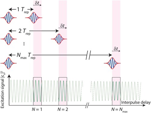
Figure 3. Example of a typical Ramsey-comb measurement in ${\mathrm{D}}_2$, for the extraction of the $\mathrm{E}\mathrm{F}(v^{\prime }=0,N^{\prime }=0)\leftarrow \mathrm{X}(v^{″}=0,N^{″}=0)$  transition frequency. Three fringes: $N=3$, 24 and 45 are recorded. The Ramsey fringe number N and interpulse delay $T_{\mathrm{r}\mathrm{e}\mathrm{p}}=1/f_{\mathrm{r}\mathrm{e}\mathrm{p}}$, set by the repetition rate $f_{\mathrm{r}\mathrm{e}\mathrm{p}}$ of the frequency comb, are scanned in a random order (top panel), and the data is then rearranged for further data analysis (bottom panel). The contrast and signal strength are high for short interpulse delays (87% at N = 3), and decrease for longer interpulse delays (43% at N = 45) due to the finite excited-state lifetime, the finite transit time of the molecules through the interaction zone and other sources of decoherence such as laser phase noise.

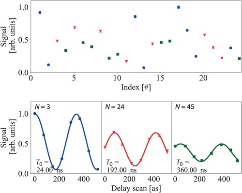
To measure the transition frequency $f_{\mathrm{t}\mathrm{r}}$, we record several so-called ‘Ramsey fringes’: i.e. we measure the excitation probability of the ${\mathrm{D}}_2$ molecules as a function of small changes of $T_{\mathrm{r}\mathrm{e}\mathrm{p}}$ (which changes $\mathrm{\Delta }t$) and repeat this for several different pulse pair combinations (different N), as shown in Figure 3. The transition frequency is then extracted by a single fit of the relative phase of all recorded Ramsey fringes.

An important aspect of Ramsey-comb spectroscopy is that spurious phase shifts in $\mathrm{\Delta }\varphi$ that are common to all Ramsey fringes drop out of the analysis, and thus do not affect the determination of the transition frequency $f_{\mathrm{t}\mathrm{r}}$ as long as they remain common-mode. This is in particular the case for differential ac-Stark shifts induced by the Ramsey-comb laser light, which we discuss in Section 3.1. The interested reader is referred to [25,26] for a more detailed description of the Ramsey-comb method and of the data analysis used to extract $f_{\mathrm{t}\mathrm{r}}$ from the recording of Ramsey fringes.

3. Experimental setup description

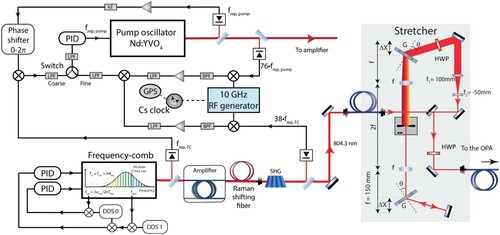
In Figure 4 a schematic overview is given of the experimental system. The system starts with the Ramsey-comb laser, followed by the upconversion to the DUV of the amplified pulses, and finishes with the vacuum setup in which ${\mathrm{D}}_2$ is excited and detected.

Figure 4. Schematic overview of the entire experimental setup. Two laser pulses from a NIR frequency comb are selectively amplified using a noncollinear optical parametric chirped-pulse amplifier (NOPCPA). The NOPCPA is driven by a pulsed pump laser, of which the repetition rate is synchronised to that of the NIR frequency comb. The pump laser produces high-intensity pulse pairs at 532 nm that are spatially and temporally overlapped with the two comb laser pulses in the beta barium borate (BBO) crystals of the NOPCPA. The resulting optical parametric amplification process leads to two NIR pulses of about 2.5 mJ (each) at the desired interpulse delay. These are then frequency-upconverted to perform the Ramsey-comb measurement in the vacuum setup on ${\mathrm{D}}_2$. Also shown is a phase measurement setup that monitors the phase influence of the NOPCPA, by combining light of the same frequency comb pulse before and after the NOPCPA.

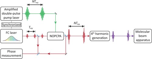
In Section 3.1, we describe the newly implemented low-phase-noise NIR frequency comb setup and locking design, followed by a brief description of the non-collinear optical parametric chirped pulse amplifier (NOPCPA, including some aspects of the pump laser for it) that produced the two amplified frequency comb laser pulses. The section concludes with a description of the phase measurement setup we implemented to monitor NOPCPA-induced (differential) phase shifts between the two amplified pulses.

In Section 3.2, we describe the upconversion of the amplified frequency comb pulses from NIR to DUV wavelengths, our new cryogenic ${\mathrm{D}}_2$ molecular beam setup, and the laser excitation and detection of the Ramsey fringes based on $\mathrm{E}\mathrm{F}(v^{\prime }=0,N^{\prime }=0)\leftarrow \mathrm{X}(v^{″}=0,N^{″}=0)$  two-photon transition of ${\mathrm{D}}_2$.

Additional technical information regarding the experimental setup is given in the Appendices section.

3.1. The near-infrared (NIR) Ramsey-comb laser system

The core principle of our NIR Ramsey-comb laser, depicted in Figure 4, is the same as in our previous work in ${\mathrm{H}}_2$ [21]: two NIR pulses from a frequency comb laser are selected by the nonlinear amplification process in a NOPCPA to obtain phase-coherent pulses with high peak intensity. The optical parametric amplification (OPA) process results in differential phase shifts between the two amplified pulses, which must be quantified and minimised. For this purpose, the phase of the amplified pulses is measured relative to the pulses entering the NOPCPA.

3.1.1. The frequency comb laser and the NIR wavelength and bandwidth selection

The frequency comb laser source is a low phase-noise FC-1500-ULN from Menlo Systems, which replaces the home-built Ti-sapphire laser frequency comb that we used in our previous work on ${\mathrm{H}}_2$ [21]. The new frequency comb laser is optically locked in the NIR, which changed the electronic locking of the rest of the system considerably. In Figure 5 an overview is given of the new configuration.

Figure 5. NIR frequency comb and pump synchronisation setup. The NIR frequency comb is optically locked to a narrow-linewidth cw laser referenced to an ultrastable optical reference cavity. The carrier-envelope offset frequency of the comb, $f_{\mathrm{c}\mathrm{e}\mathrm{o}}$, is locked to the 50 MHz output of a Direct Digital Synthesizer (DDS) referenced to a caesium atomic clock. The repetition rate of the pump laser oscillator (125 MHz) is locked to half the repetition rate of the frequency comb (250 MHz) to ensure timing overlap of the pulses from the systems in the NOPCPA, where the frequency comb pulses are amplified. Both ${\mathrm{f}}_{\mathrm{r}\mathrm{e}\mathrm{p}}$ and $f_{\mathrm{c}\mathrm{e}\mathrm{o}}$ are recorded during the Ramsey-comb measurements. The fundamental wavelength of the comb is shifted from 1550 nm to 1600 nm with a Raman-shifting fibre, after which the entire spectrum is frequency doubled to 804.32 nm, required for further upconversion to 201.08 nm for ${\mathrm{D}}_2$ spectroscopy. A 4f-grating stretcher with spectral filtering selects the central wavelength and bandwidth, and sets a frequency comb pulse duration of 7 ps, which is optimal for NOPCPA amplification with 48 ps pump pulses. Half-wave plates (HWP) enable optimisation of the polarisation for the gratings and for the single-mode polarisation maintaining fibre going to the NOPCPA.

The frequency comb has a central wavelength of 1550 nm, an offset frequency $f_{\mathrm{c}\mathrm{e}\mathrm{o}}$ of 50 MHz and a repetition rate $f_{\mathrm{r}\mathrm{e}\mathrm{p}}$ of 250 MHz. The offset frequency is locked to the output of a Direct Digital Synthesizer (DDS) that is referenced to a Cs atomic clock. The repetition rate is set indirectly as the frequency comb laser is optically locked near 1542 nm, to a sub-2 Hz-linewidth cw reference laser at the same wavelength (ORS1500, Menlo Systems). This lock, with one of the comb teeth near 1542 nm, is maintained at an offset produced by a DDS (also referenced to the caesium atomic clock). The resulting repetition rate of the comb is measured with a photodiode and counted relative to the Cs clock. Adjustments to the DDS are made to achieve the targeted $f_{\mathrm{r}\mathrm{e}\mathrm{p}}$ for scanning of the Ramsey fringes. This method enables us to combine the stability of optically locking a frequency comb with the requirement of scanning the repetition rate to record Ramsey fringes.

The central wavelength of the frequency comb laser output needs to be adjusted for the ${\mathrm{D}}_2$ experiment. It is red-shifted from 1550 nm to 1600 nm using a Raman-shifting fibre, and then frequency-doubled in a periodically-poled lithium niobate fanout crystal to achieve maximum power spectral density at 804.32 nm. This is required to perform ${\mathrm{D}}_2$ spectroscopy at 201.08 nm after frequency-upconversion to the DUV–see Section 3.2.1. For optimal OPA amplification and selection of the proper wavelength, the 240 fs NIR pulses from the frequency comb laser are sent into a 4-f, double-grating stretcher (see Figure 5). There they are chirped and filtered spectrally (with a slit in the Fourier plane) to a bandwidth of 0.2 nm at a central wavelength of 804.32 nm, to make sure that only the $\mathrm{E}\mathrm{F}(v^{\prime }=0,N^{\prime }=0)\leftarrow \mathrm{X}(v^{″}=0,N^{″}=0)$  two-photon transition at 201.08 nm ($Q_0$ transition) is excited and not e.g. the $Q_1$ transition at 201.14 nm–see Figure 1. A 10 m long polarisation-maintaining single-mode fibre is used to transport the NIR pulses to the amplification optical table, and together with the group delay dispersion (GDD) of about 10${}^6$ fs${}^2$ from the stretcher, this results in 7 ps pulse length and 1 pJ pulse energy before amplification in the NOPCPA.

3.1.2. The two-pulse parametric amplifier system (NOPCPA)

The noncollinear optical parametric chirped-pulse amplifier system follows the design presented in [31], in which two NIR frequency comb pulses and two 532 nm pump laser pulses are combined in BBO crystals in a noncollinear fashion. This results in optical parametric amplification of the frequency comb pulses, which draw energy from the pump laser pulses. The (stretched) frequency comb and pump pulse durations of 7 ps and 48 ps, respectively, are chosen to ensure a good balance between amplification efficiency and stability. What follows is a brief description of the NOPCPA, while details of the pump laser can be found in the Appendix 1.

Two successive amplification stages can be distinguished in the NOPCPA. The first amplification stage consists of two BBO crystals, pumped with low-power 532 nm pump pulse pairs of about 1 mJ per pulse. A small beam size (<1 mm diameter) is used to ensure a sufficiently high pump intensity of about 3 GWcm${}^{-2}$ in the crystals, for optimal energy transfer. Due to walk-off in the BBO crystals, an intensity-dependent wavefront tilt is induced on the amplified pulses which is detrimental to high-precision spectroscopy. This is compensated for by rotating the optical axis of the second crystal with respect to the first one, as explained in [31]. The second amplification stage consists of a single BBO crystal, pumped with high-power 532 nm pulse pairs of about 20 mJ/pulse and a larger pump beam diameter (4–5 mm) to minimise wavefront and beam profile inhomogeneities during the OPA amplification process.² Each of the two amplified frequency comb pulses reaches an energy of about 2.5 mJ at the output of the second stage of the NOPCPA. At this point the amplified beam resembles the top-hat intensity profile of the pump beam. Therefore an in-vacuum 300-micron spatial filter is used to convert the beam to a Gaussian intensity profile again, leaving 1.5 mJ per pulse for frequency upconversion and spectroscopy.

The long-term intensity stability of the amplified NIR pulses is about 5% over a day, with short-term rms fluctuations of the pulse ratio of 1–1.5%. Averaged over a Ramsey fringe, the NOPCPA output energy is typically constant to 0.1%. This is achieved by stabilisation of the energy of the pump pulses (see A.1). It is important to keep the averaged pulse energy over the Ramsey fringe constant to minimise variations of the ac-Stark phase shifts between Ramsey fringe recordings.

3.1.3. Measurement of the NOPCPA-induced amplification phase shifts

The OPA amplification process described in the previous section can lead to a temporal phase shift ${\varphi }_{\mathrm{a}\mathrm{m}\mathrm{p}}$ of the amplified pulses relative to the original frequency comb laser pulses. It is important to realise that only the difference in phase shift between the two pulses matters. So if the differential amplification phase shift ${\varphi }_{\mathrm{a}\mathrm{m}\mathrm{p},\mathrm{p}\mathrm{u}\mathrm{l}\mathrm{s}\mathrm{e}2}-{\varphi }_{\mathrm{a}\mathrm{m}\mathrm{p},\mathrm{p}\mathrm{u}\mathrm{l}\mathrm{s}\mathrm{e}1}$ experienced by the pair of Ramsey comb excitation pulses is constant for all Ramsey fringes (all N), then it has no influence as it will show up in the signal as a common phase shift. But if there is an N dependence, it will lead to an effective delay-dependent phase shift and thus to an error in the determination of the transition frequency–see Section 2. For this reason, the differential phase shift as a function of N needs to be determined.

We use an interferometric phase measurement setup to measure and account for the NOPCPA-induced differential amplification phase shifts for all Ramsey fringes. It is depicted in Figure 6. The principle is based on spectral interferometry. Before the NOPCPA, a little bit of power of the original frequency comb pulses is split-off and later recombined with the amplified pulses. Transmission through a single-mode fibre is used to ensure perfect spatial overlap. A small delay of about 1 ps is applied between the amplified and the original pulses and this produces a spectral interference pattern in the frequency domain. A diffraction grating and optics are then used as a high-resolution spectrometer to monitor this pattern. Two interference patterns are produced, one for each of the two Ramsey-comb pulses. With a Pockels cell and polarisation optics we project them onto a camera above each other–see the camera picture in Figure 6. The phase of the patterns depends on the time delay and phase difference of the two interfering pulses. A comparison of the two interference patterns yields the phase shift $\mathrm{\Delta }\varphi =N\times {\varphi }_{\mathrm{c}\mathrm{e}\mathrm{o}}+{\varphi }_{\mathrm{a}\mathrm{m}\mathrm{p},\mathrm{p}\mathrm{u}\mathrm{l}\mathrm{s}\mathrm{e}2}-{\varphi }_{\mathrm{a}\mathrm{m}\mathrm{p},\mathrm{p}\mathrm{u}\mathrm{l}\mathrm{s}\mathrm{e}1}$ between the two amplified pulses and thus to the differential amplification phase shift,³ equal to ${\varphi }_{\mathrm{a}\mathrm{m}\mathrm{p},\mathrm{p}\mathrm{u}\mathrm{l}\mathrm{s}\mathrm{e}2}-{\varphi }_{\mathrm{a}\mathrm{m}\mathrm{p},\mathrm{p}\mathrm{u}\mathrm{l}\mathrm{s}\mathrm{e}1}$. The measured phase difference between the two patterns is in part due to the geometry and alignment of the two interference patterns. By exchanging the projection of both pulses (using Pockels cell PC3 in Figure 6), this geometrical phase shift can be eliminated and the pure differential phase shift of the amplified pulses relative to the original frequency comb pulses can be obtained. The outcome of a typical phase measurement is shown in Figure 7. For more details of the procedure, see the Appendix 2.

Figure 6. Phase measurement setup for the monitoring of NOPCPA-induced differential amplification phase shifts. The phase measurement is based on spectral interferometry. Part of the amplified frequency comb pulses are combined with their corresponding reference frequency comb pulses in a single-mode fibre to ensure perfect spatial overlap. Two Pockels cells (PC1 and PC2), in combination with polarisation beam splitters, suppress the non-amplified background pulses. A third Pockels cell (PC3) selects one of the amplified/non-amplified pulse combinations and displaces it vertically compared to the other pulse combination. The pulses are then sent onto a gold diffraction grating and are imaged onto an image intensifier ('Cricket' from Photonis) and CMOS camera (Manta G-235B from Allied Vision) to detect the interference pattern associated with each pulse.

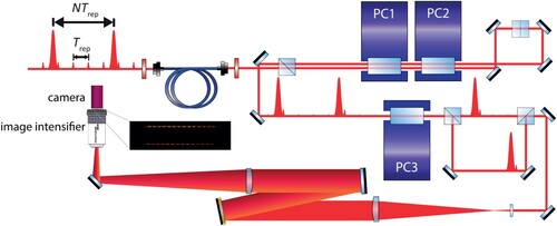
Figure 7. Typical differential phase measurement of the amplified frequency comb pulses, at a pulse bandwidth of 4.5 nm. A linear fit is performed to extract the phase shift with respect to the interpulse delay. This example measurement shows a time delay-dependent slope in relative phase shift of 0.103(0.071) mrad per 8 ns ($\mathrm{\Delta }N=1$), which results in a frequency shift of 16.4(11.3) kHz on the observed transition frequency in the DUV.

The measured differential amplification phase shifts at 808 nm are typically on the order of −50 to 50 mrad, depending on the daily NOPCPA alignment. The phase noise is usually between 20 to 80 mrad.

3.2. Deep-UV laser excitation in a beam of ${\mathrm{D}}_2$ molecules

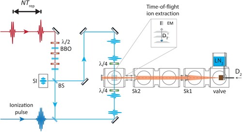
The two-photon $\mathrm{E}\mathrm{F}(v^{\prime }=0,N^{\prime }=0)\leftarrow \mathrm{X}(v^{″}=0,N^{″}=0)$  laser excitation is performed in a cold and slow beam of ${\mathrm{D}}_2$ molecules, using counter-propagating DUV laser beams to reduce the first-order Doppler shift–see Figure 8. The most important aspects of DUV production, excitation geometry and excited state detection are explained below.

Figure 8. Deep-UV laser excitation and detection setup for Doppler-free Ramsey-comb spectroscopy. The NOPCPA-amplified NIR frequency comb pulses are frequency-upconverted from 804.32 to 201.08 nm in three BBO crystals. The DUV pulses are then split in two different paths by a metallic beam splitter (BS) and recombined onto a cold and slow ${\mathrm{D}}_2$ molecular beam in a Doppler-free counter-propagating excitation geometry (both paths towards the molecular beam are in reality equal in length). A 355 nm laser pulse selectively ionises those molecules that have been excited successfully to the EF state, 5 ns after the second Ramsey-comb excitation pulse. The resulting ions are then sent through a time-of-flight mass spectrometer (with a pulsed field that is switched on just after the ionisation pulse to minimise dc-Stark effects) and then detected with an electron multiplier (EM). The beam splitter also forms the exit port of a Sagnac interferometer (SI), which is used to monitor the relative alignment of the two counterpropagating beams. Sk1 is a skimmer with 3 mm opening, and Sk2 has an opening of 8 mm.

3.2.1. DUV generation and the laser excitation geometry

The two NOPCPA-amplified NIR frequency comb pulses for the Ramsey-comb measurement (see Section 3.1) are upconverted to the DUV in three stages using type-I phase matching in three BBO crystals. In the first BBO crystal, part of the power of the original fundamental NIR pulses at 804.32 nm is frequency doubled to 402.16 nm. The second crystal then combines the 402.16 nm with some of the remaining 804.32 nm to produce the third harmonic, and in the third BBO crystal this is mixed again with the fundamental to produce 201.08 nm. Special half-wave plates from B. Halle are used to rotate selectively the polarisation of the light at the newly-created wavelengths (402.16 and 268.11 nm) in between each crystal while keeping the polarisation of the NIR fundamental light the same, so as to enable type-I phase matching throughout.

Because of the two-photon nature of the $\mathrm{E}\mathrm{F}(v^{\prime }=0,N^{\prime }=0)\leftarrow \mathrm{X}(v^{″}=0,N^{″}=0)$  transition, it is possible to suppress the first-order Doppler effect with counter-propagating laser beams. For this purpose, the DUV beam is split in equal parts by a metallic beam splitter. The finite bandwidth of the excitation pulses does limit the Doppler-cancellation effect, and therefore special care was taken to align both beams such that they propagate as much as possible perpendicularly to the ${\mathrm{D}}_2$ molecular beam. The two beams then meet spatially and temporally at the location of the ${\mathrm{D}}_2$ molecules.⁴ This configuration reduces the first-order Doppler shift by about 3 orders of magnitude compared to a collinear geometry. A quarter-wave plate in each excitation path changes the polarisation of the DUV light from linear to circular, which suppresses one-sided collinear absorption by a factor of 10. After the excitation zone, both beams continue and arrive again at the beam splitter. The exit port of this beam splitter acts as a Sagnac interferometer, which can be used to align the excitation beams [32]. With perfect counter-propagating DUV beams, all output at the beam splitter is suppressed (a dark fringe). This effect is used to align the excitation beams counter-propagating with an accuracy of 70 μrad.

The DUV single-pulse energy is set to 54 $\mu$J (with an estimated day-to-day reproducibility of 5% and an absolute accuracy of 10%) to perform the ${\mathrm{D}}_2$ Ramsey-comb measurements. The stability of the averaged DUV pulse energy over a full Ramsey fringe, as function of the macro-delay N, determines how much residual ac Stark shift is observed. We therefore tried to make it as stable as possible, but it was difficult to determine the actual stability because the DUV light caused damage to the photodiodes. To still get an estimate, we take the averaged NOPCPA output (NIR) stability per Ramsey fringe of 0.1% (see A.1), and assume that the DUV is varying roughly 4 times more (linear regime of upconversion). This leads to an estimated average pulse-energy stability over a full Ramsey fringe of 1.2% in the DUV. However, this number does not affect any of the results, as the differential ac-Stark shift has been measured directly (Section 4.2.2).

We use a DUV pulse duration of 7 ps (see Section 3.1.1) and a FWHM (Gaussian) beam diameter of 1 mm at the interaction zone, which gives a single-pulse DUV intensity of about $2.4\times {10}^8$ Wcm${}^{-2}$ for each of the two Ramsey-comb excitation pulses.

3.2.2. Production of a cold and slow beam of ${\mathrm{D}}_2$ molecules

Excitation takes place in a supersonic beam of cold ${\mathrm{D}}_2$ molecules, as depicted on the right side of Figure 8. The molecular beam apparatus has been improved since the last Ramsey-comb measurements in ${\mathrm{H}}_2$ [21], leading to a higher molecular density and a reduction of the beam divergence (for extra information see A.3). This has improved both the signal strength and the Ramsey-fringe contrast.

The most important change compared to our previous work is the use of a new pulsed molecular valve, developed in the group of Prof. Dr. F. Merkt at the ETH Zürich. This valve can produce very short, high-density pulses of 29 $\mu$s duration, 10 times shorter than with the valve we used before. It is cooled with a liquid nitrogen reservoir to about 110 K by thermal contact, slowing down the ${\mathrm{D}}_2$ molecules from 1940 m/s at room temperature to 999(29) m/s when cooled down.⁵ To further decrease the velocity of the molecules, we use a mixture of 2 parts of ${\mathrm{D}}_2$ mixed with 3 parts Ne (see Appendix 3). The collisions of the ${\mathrm{D}}_2$ molecules with the neon atoms slow down the ${\mathrm{D}}_2$ molecules by another factor of two, to 571(13) m/s.

Decreasing the velocity of the ${\mathrm{D}}_2$ molecules improves the contrast of the Ramsey fringes for larger interpulse delays (higher N, see Figure 3) and thus enables a better experimental accuracy in general. The reason is that at lower velocities, the molecules remain within the excitation beams even for long interpulse delays, so that the phase evolution of the excited superposition state can be measured more accurately. Moreover, the less the molecules move, the less sensitive the excitation process is to laser wavefront imperfections, like non-ideal DUV beam collimation. With the new valve installed, we can perform Ramsey-comb measurements with interpulse delays extending up to $N=45$ ($\mathrm{\Delta }t=360$ ns) for both pure ${\mathrm{D}}_2$ and the 2${\mathrm{D}}_2$:3Ne mixture, limited mostly by the 200 ns excited-state lifetime of the $\mathrm{E}\mathrm{F}(v^{\prime }=0,N^{\prime }=0)\leftarrow \mathrm{X}(v^{″}=0,N^{″}=0)$  transition. The longest pulse delay is significantly shorter than the molecular transit time in the interaction zone–it takes respectively 1.0 $\mu$s and 1.8 $\mu$s for the ${\mathrm{D}}_2$ molecules to go through the 1 mm beam diameter of the DUV excitation beams at 999 m /s and 571 m/s –, therefore we conclude that transit-time limitations are now virtually absent from our ${\mathrm{D}}_2$ measurements.

3.2.3. Detection of the $\mathrm{E}\mathrm{F}(v^{\prime }=0,N^{\prime }=0)\leftarrow \mathrm{X}(v^{″}=0,N^{″}=0)$  two-photon excitation

Detection of molecules excited to the EF state is done using state-selective ionisation and time-of-flight ion extraction, as shown in Figure 8. The ${\mathrm{D}}_2$ molecules that have been successfully excited to the EF state after the Ramsey-comb sequence are ionised by a 355 nm laser pulse of 48 ps duration and 0.6 mJ pulse energy. The 355 nm ionisation pulse is derived from the leftover non-frequency-doubled 1064 nm light generated by the pump laser of the NOPCPA. Only the second of the two 1064 nm pump pulses is selected with a Pockels cell and polarising optics. The selected pulse is then upconverted to the third harmonic using two nonlinear crystals (Quanta-Ray Harmonic Generator, model Hg-2). The length of the beam path is adjusted such that the ionisation pulse arrives 5 ns after the second excitation pulse in the interaction zone, to avoid any light shift induced by the ionisation beam. The ions are extracted in a time-of-flight mass spectrometer with a voltage difference of 50 V applied on two plates (separated by 17 mm) around the interaction zone. This electric field is applied 5 ns after the second excitation pulse to avoid dc-Stark shifts during laser excitation, and it is kept on for a duration of 1 $\mu$s. The ions are then pulled in a field-free drift tube which has an electron multiplier at the end to detect the ions. The signal from this detector is proportional to the population of the excited $\mathrm{E}\mathrm{F}$ state of ${\mathrm{D}}_2$, $|c_e\left(t\right){|}^2$ (see Equation (3(3) $|c_{\mathrm{e}}\left(t\right){|}^2\propto 1+\cos (2\pi f_{\mathrm{t}\mathrm{r}}\mathrm{\Delta }t-\mathrm{\Delta }\varphi ),$(3) )), which is recorded for further data analysis.

4. The ${\mathrm{D}}_2$ spectroscopy results

With the setup described in the previous section, we have determined a new value for the $\mathrm{E}\mathrm{F}(v^{\prime }=0,N^{\prime }=0)\leftarrow \mathrm{X}(v^{″}=0,N^{″}=0)$  transition frequency, equal to $f_{\mathrm{t}\mathrm{r}}=2,981,779,227,578$ kHz with an accuracy of 19 kHz. The determination of the transition is performed in several steps.

In Section 4.1, we describe the experimental method and the data analysis procedure that we use to first determine a transition frequency corrected for only the first-order Doppler effect and for residual NOPCPA-induced amplification phase shifts. In Section 4.2, we discuss the additional systematic effects that contribute to the error budget and the corrections associated with it: the systematic offset of the phase measurement setup, the second-order Doppler effect, the differential ac-Stark shifts (light shifts) induced on the ${\mathrm{D}}_2$ transition by the Ramsey-comb laser pulses, the dc-Stark shift induced by a residual voltage on the ion-extraction plates, the Zeeman effect, and the offset of the atomic clock reference. The contribution of each of these effects is summarised in Table 2. Other systematic effects, such as the ac-Stark shift induced on the transition by ambient black-body radiation or the hyperfine structure of ${\mathrm{D}}_2$ (see Section 4.2.6 below), are not significant at our measurement accuracy. Additional information regarding the data taking and data processing is given in Appendix 4.

Table 2. Determination of the $\mathrm{E}\mathrm{F}(v^{\prime }=0,N^{\prime }=0)\leftarrow \mathrm{X}(v^{″}=0,N^{″}=0)$  transition frequency in molecular deuterium, including all corrections and uncertainties.

	Value or correction (kHz)	Uncertainty (kHz)
First-order Doppler-free and
amplifier-phase-shift corrected frequency	2,981,779,227,585	13
Corrections
Second-order Doppler	−9	2
ac-Stark shift	9	14
Phase measurement setup offset	−6	2
Zeeman shift	0	1
Cs clock	−1	0.15
dc-Stark shift	0	1
Total	2,981,779,227,578	19

4.1. Determination of the Doppler-free transition frequency

4.1.1. Experimental procedure

We determine the first-order Doppler-free $\mathrm{E}\mathrm{F}(v^{\prime }=0,N^{\prime }=0)\leftarrow \mathrm{X}(v^{″}=0,N^{″}=0)$  transition frequency by combining Ramsey-comb measurements performed with pure ${\mathrm{D}}_2$ gas at a mean velocity of 999(29) m/s, with those based on a 2D${}_2$:3Ne mixture with a mean velocity 571(13) m/s (see Section 3.2.2). Both measurements are performed with the ${\mathrm{D}}_2$ valve cooled down to 110K by thermal contact with liquid nitrogen. Previously, we changed the velocity by changing the temperature of the valve [21], but this took 30 minutes. Instead, because we now only switch between pure ${\mathrm{D}}_2$ and the mixture of ${\mathrm{D}}_2$ with neon, we can change the speed of the ${\mathrm{D}}_2$ beam in about 5 minutes. This makes the measurements less susceptible to drift effects and improves the determination of the residual first-order Doppler shifts.

Each Ramsey-comb measurement consists of three recorded Ramsey fringes, at N = 3, 24 and 45, corresponding to a given pulse pair combination and an interpulse delay (macro-delay) $\mathrm{\Delta }t=N\times T_{\mathrm{r}\mathrm{e}\mathrm{p}}$, as shown in Figures 2 and 3. For each N, a micro-delay $\delta t$ is scanned in 8 points over 500 attoseconds (as) to record a Ramsey fringe by changing the repetition rate $f_{\mathrm{r}\mathrm{e}\mathrm{p}}=1/T_{\mathrm{r}\mathrm{e}\mathrm{p}}$ of the frequency comb at a level of 20.8 ppb for N = 3, and only 1.36 ppb for N = 45. Both N and $f_{\mathrm{r}\mathrm{e}\mathrm{p}}$ are scanned in a random order, and three Ramsey-comb measurements are performed for each of the two ${\mathrm{D}}_2$ velocities. The average of the three extracted frequencies is then used to extract the first-order Doppler-free transition frequency by linear extrapolation to zero velocity. An example is shown in Figure 9. We performed in total 25 of such Doppler-free extrapolations, corresponding to 150 Ramsey-comb measurements over the course of 5 days.

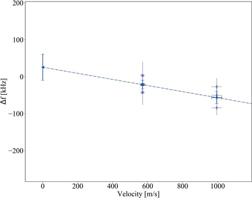
Figure 9. Example of an extrapolation to zero velocity of the first-order residual Doppler shift on the $\mathrm{E}\mathrm{F}(v^{\prime }=0,N^{\prime }=0)\leftarrow \mathrm{X}(v^{″}=0,N^{″}=0)$  $Q_0$ transition in ${\mathrm{D}}_2$. The extrapolation is based on two sets of 3 measurements, one set performed with pure ${\mathrm{D}}_2$ gas with a mean velocity of 999(29) m/s, and the other with a 2D${}_2$:3 Ne mixture that has a mean ${\mathrm{D}}_2$ velocity of 571(13) m/s.

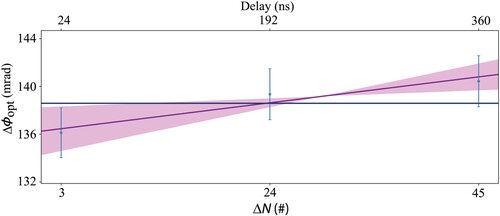
We correct each Doppler-free frequency determination for the NOPCPA-induced differential amplification phase shifts using the method described in Section 4.2.1. The amplifier phase shift is measured daily, before and after the Ramsey-comb Doppler-free measurements.⁶ We do this for each value of N and $T_{\mathrm{r}\mathrm{e}\mathrm{p}}$ that we use for the actual Ramsey-comb measurements, also in random order and for a total number of phase measurements which is half that of the number of Ramsey-comb measurements of a given day. We then perform a linear fit of the phase shifts with respect to the interpulse delay $\mathrm{\Delta }t=\mathrm{\Delta }N\times T_{\mathrm{r}\mathrm{e}\mathrm{p}}$, and extract the effective interpulse-delay dependent phase shift $\mathrm{\Delta }{\varphi }_{\mathrm{a}\mathrm{m}\mathrm{p}}/(\mathrm{\Delta }N\times T_{rep})$ from the slope of the fit. An example is shown in Figure 10, where measurements before (on the left of the vertical line) and after (on the right of the vertical line) the Ramsey-comb measurements of a given day are presented. The average phase slope (equivalent to the frequency shift) is then used to determine the effective frequency shift with which the corresponding daily averaged Doppler-minimised measurements must be corrected using Equation (A1) (see Appendix 2). The result is shown in Figure 11 for the five measurements days.

Figure 10. Example of NOPCPA-induced amplification phase shift measurements as measured before (left of the vertical line) and after (right of the vertical line) the Ramsey-comb measurements used for the determination of the first-order Doppler-free transition frequency. For the phase measurement, the same micro-delays and inter-pulse delays were used as during the spectroscopy. The averaged frequency shift of −29.7(15.3) kHz, calculated from these measurements, is used to correct the first-order Doppler-free transition frequency obtained on that day. The error bar from the fit of the individual phase shift measurements is not plotted because the observed variations are several times larger due to external influences. Therefore the uncertainty on the calculated averaged frequency shift correction is directly derived from the variation of the phase measurements with equal weight for all data points.

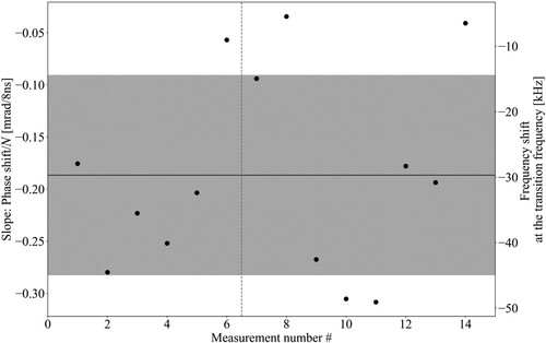
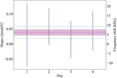
Figure 11. First-order Doppler-free transition frequency determination for each measurement day of the $\mathrm{E}\mathrm{F}(v^{\prime }=0,N^{\prime }=0)\leftarrow \mathrm{X}(v^{″}=0,N^{″}=0)$  $Q_0$ transition in ${\mathrm{D}}_2$. The frequency is given relative to an offset frequency of −2 MHz with respect to the previously determined value [24]. The first-order Doppler-free frequency is corrected for the amplifier phase shift and averaged over 5 days to reach a statistical accuracy of 13 kHz (shown by the pink band as the weighted standard error). The dotted line shows the weighted standard deviation at 30 kHz. During the measurement campaign, the nonlinear crystals for DUV generation deteriorated, resulting in reduced measurement statistics and making it progressively harder to continue the experiment. In particular, during the last measurement day, the signal strength and contrast were much lower.

After correcting all Doppler-free extrapolations for the NOPCPA phase shift in this fashion, the values are averaged to obtain the first-order Doppler-free and amplifier phase-shift corrected value listed in Table 2. The second-order Doppler effect is discussed in the next section, and further corrections are discussed in Section 4.2.

4.1.2. The second-order Doppler effect

In the correction procedure for the first-order Doppler effect, the second-order Doppler effect due to the absolute velocity was not taken into account. We compensate for this afterwards. As the second-order Doppler effect is equal to $\mathrm{\Delta }{f}_{\mathrm{t}\mathrm{r},2\mathrm{n}\mathrm{d}-\mathrm{o}\mathrm{r}\mathrm{d}\mathrm{e}\mathrm{r}\mathrm{D}\mathrm{o}\mathrm{p}\mathrm{p}\mathrm{l}\mathrm{e}\mathrm{r}}=-\frac{v^2}{2c^2}{f}_0$, the observed transition frequency is shifted down 16.75 kHz for pure ${\mathrm{D}}_2$ gas at a velocity of 999 m/s, and 5.41 kHz down for the 2${\mathrm{D}}_2$:3Ne mixture at 571 m/s. In the linear extrapolation to zero velocity of the first-order shift, this leads to a upward shift of 9 kHz compared to the true transition frequency. Therefore a −9(2) kHz correction to the frequency obtained from the first-order Doppler-free extrapolations is applied, listed as Second-order Doppler in Table 2, to obtain the true transition frequency.

4.1.3. Lifting the ambiguity on the determination of the transition frequency

It should be noted that Equation (3(3) $|c_{\mathrm{e}}\left(t\right){|}^2\propto 1+\cos (2\pi f_{\mathrm{t}\mathrm{r}}\mathrm{\Delta }t-\mathrm{\Delta }\varphi ),$(3) ) is periodic, which results in the extraction of a series of possible transition frequencies. The frequency periodicity (ambiguity) is $f_{\mathrm{r}\mathrm{e}\mathrm{p}}/\mathrm{\Delta }N$, where $\mathrm{\Delta }N$ corresponds to the interpulse delay jumps between the Ramsey-fringes. For the correct determination, we therefore performed Ramsey-comb spectroscopy also with a smaller macro-delay jump (between $\mathrm{\Delta }N=1$ and $\mathrm{\Delta }N=3$ instead of $\mathrm{\Delta }N=21$) as a means of reducing the set of possible transition frequencies. A Ramsey-comb measurement with $\mathrm{\Delta }N=3$ is shown in Figure 12(a) with its Fourier transform in part (b). The Fourier transform of the fringes clearly shows the possible frequencies where the transition could be. The real one can be identified by comparing it with a previous measurement. For this purpose the value from [24] is indicated by the vertical lines in Figure 12(b) with an uncertainty of 3.3 MHz (shown by the dashed vertical lines). The distance of the possible transition frequencies to the previously determined transition frequencies shows that we can attribute the signal clearly to the $Q_0$ transition.

Figure 12. (a) Identification of the ${\mathrm{D}}_2$ transition by an overview scan of Ramsey fringes obtained for different pulse pair combinations N, associated with the macro-delay $\mathrm{\Delta }t=N\times T_{\mathrm{r}\mathrm{e}\mathrm{p}}$. The maximum interpulse delay recorded is $\mathrm{\Delta }t=360$ ns, corresponding to N = 45. The measurement data are shown in blue. The red fit is performed on each Ramsey fringe while the green fit uses all fringes with an exponentially decaying amplitude to account for the contrast loss at higher N. (b) The Fourier transformation of 35 Ramsey-fringes. An interpulse delay spacing of $\mathrm{\Delta }N=3$ between the Ramsey-fringes is used to discriminate between all possible values of the transition frequencies modulo $f_{\mathrm{r}\mathrm{e}\mathrm{p}}/\mathrm{\Delta }N$ (41.7 MHz in this case). The blue curve corresponds to the Fourier transform of the data while the red one corresponds to the Fourier transform of the fit. The difference is shown by the violet curve. The vertical lines represent the values of the corresponding transition frequency determined in [24]. The corresponding uncertainties (1σ) are shown by the dashed lines. The Fourier peak coincides with the previous $Q_0$.

4.2. Additional systematic effects

4.2.1. Phase measurement setup offset

The phase measurement setup (see Section 4.2.1) to monitor NOPCPA-induced phase shifts can have a systematic offset. The origin is the small pulse delay (1 ps) between the original and amplified pulses, required to generate a spectral interference pattern, in combination with the finite switching speed of a few ns of the Pockels cells. We determine this potential offset by performing a self-reference measurement where the reference pulses interfere with themselves. In this case, the stretched frequency comb pulses are split into two almost identical beam paths before they are recombined in the single-mode fibre that forms the entrance to the phase measurement. Any measured interpulse-delay dependent relative phase shift then arises from the phase measurement setup itself, and not from the amplification of the frequency comb pulses. In Figure 13 the self-referenced phase measurements are presented. There is a small but persistent delay-dependent phase shift present in all measurements, and a correction must be applied for it. In total 80 self-reference phase measurements were performed over 4 days. After averaging these measurements, this leads to a correction of −6(2) kHz on the transition frequency, as listed under Phase measurement setup offset in Table 2.

Figure 13. Self-reference phase measurements, used to quantify the systematic error induced by the phase measurement setup itself. The effective frequency shift due to the offset from zero is equivalent to 6(2) kHz in the DUV, and must be subtracted from the determined transition frequency.

4.2.2. The ac-Stark shift by the DUV excitation beam

The ${\mathrm{D}}_2$ molecules experience a very strong ac-Stark shift (light shift) on the $\mathrm{E}\mathrm{F}(v^{\prime }=0,N^{\prime }=0)\leftarrow \mathrm{X}(v^{″}=0,N^{″}=0)$  transition during the brief moment that the two high-intensity DUV excitation pulses interact with the molecules.⁷ However, as long as the differential ac-Stark shift ${\varphi }_{\mathrm{a}\mathrm{c}-\mathrm{S}\mathrm{t}\mathrm{a}\mathrm{r}\mathrm{k}2}-{\varphi }_{\mathrm{a}\mathrm{c}-\mathrm{S}\mathrm{t}\mathrm{a}\mathrm{r}\mathrm{k}1}$ between the two Ramsey-comb excitation pulses is constant for all Ramsey fringes (all N), its effect drops out as a common-mode phase shift to which Ramsey-comb spectroscopy is insensitive–see Section 2. This is largely the case for our ${\mathrm{D}}_2$ spectroscopy since we stabilise the intensity ratio and the total energy of the pulses as described in Section A.1. Even so, residual N-dependent deviations of the pulse energy can still translate into a frequency shift of the measured transition frequency. Moreover, the molecules move to a different position in the DUV beam between the two excitation pulses, so that they could experience a different intensity. Most of this effect will average away over the total ensemble of molecules, but a residual shift could still remain.

We quantify experimentally the residual ac-Stark shifts by performing Ramsey-comb spectroscopy for two DUV excitation energies: 63 $\mu$J and 23 $\mu$J per pulse, both with a relative accuracy of 5%. One Doppler-free frequency determination is performed for each of the two excitation energies, as described in Section 4.1, and a linear fit between these two points gives an estimate of the residual (linear) ac-Stark shift $\mathrm{\Delta }{f}_{\mathrm{a}\mathrm{c}-\mathrm{S}\mathrm{t}\mathrm{a}\mathrm{r}\mathrm{k}}\left(E\right)=\alpha \times E$, where α is the slope obtained from the fit and E is the single pulse energy.⁸ The frequency shift is then evaluated at a pulse energy of 54 $\mu$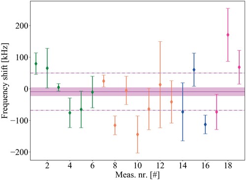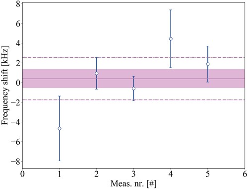J for each data set, which corresponds to the pulse energy we used in the Ramsey-comb measurements to determine the first-order Doppler-free transition frequency (see Section 3.2). The average shift is −9(14) kHz, based on a total of 20 Ramsey-comb measurements, as shown in Figure 14. The displayed uncertainty corresponds to the weighted standard error.

Figure 14. Determination of the ac-Stark shift on the transition frequency by evaluating the shift of the transition frequency at 54(3) $\mu$J /pulse (at which the first-order Doppler-free measurements were performed) based on a linear interpolation of transition frequencies at 23(1) $\mu$J/pulse and 63(3) $\mu$J /pulse. These measurements were performed over 4 days, where each point in the graph is based on at least three sets of ac-Stark measurements, that in turn are each based on 3 Ramsey-comb measurements at both low and high pulse energy. The weighted average over all measurements results in an ac-Stark shift of −9(14) kHz from the 201 nm excitation pulses, with the standard error shown by the pink band. The pink dotted line shows the weighted standard deviation of 59 kHz, and the different colours of the data points represent different days.

4.2.3. The dc-Stark shift

The ${\mathrm{D}}_2$ molecule does not have a permanent dipole moment, due to its homonuclear nature, and is therefore not sensitive to the linear dc-Stark effect. We nevertheless evaluated a possible higher-order shift by comparing Ramsey-comb measurements performed in a high static electric field of 29.4 V/cm in the interaction zone (by putting a constant voltage on the ion extraction plates), with measurements at near-zero electric field (based on the pulsed extraction field as we do for regular Ramsey-comb measurements, see Section 3.2.3). In the case of the pulsed extraction field, there was only a small residual field in the interaction zone during excitation of −1.2 V/cm. Based on the transition frequencies measured at these low and high electric fields, we infer a dc-Stark shift of 0(1) kHz for the regular measurements, consistent with zero, as shown in Figure 15.

Figure 15. The dc Stark effect on the $\mathrm{E}\mathrm{F}(v^{\prime }=0,N^{\prime }=0)\leftarrow \mathrm{X}(v^{″}=0,N^{″}=0)$  $Q_0$ transition in ${\mathrm{D}}_2$ due to a residual electric field of -1.2 V/cm in the interaction zone. This is determined based on a comparison with measurements at high electric field (29.4  V/cm), and it is consistent with zero. The violet band represents the weighted standard error equal to 1 kHz while the dashed line shows the weighted standard deviation of 2 kHz.

4.2.4. Zeeman effect

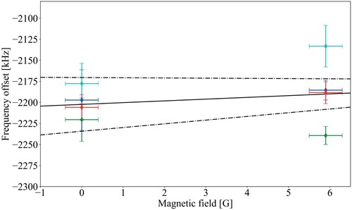
To first approximation, one expects the rotational ground state of the X and EF electronic levels to show the same Zeeman effect. Assuming an equal population of all Zeeman components in the experiment, no (first-order) Zeeman shift is then expected for the $\mathrm{E}\mathrm{F}(v^{\prime }=0,N^{\prime }=0)\leftarrow \mathrm{X}(v^{″}=0,N^{″}=0)$  transition. To verify this assumption, we compared the transition frequency measured in a low magnetic field situation, where we compensated the Earth's magnetic field in the interaction zone, to the frequency obtained when we apply an external field of either 4 G and 6 G parallel or perpendicularly, respectively, to the polarisation axis of the DUV excitation beams. In Figure 16, the measurements for a perpendicular field are shown. Each data point is the result of 3 Ramsey-comb measurements at either low (0 G) or high (6 G) field, and a linear regression was performed for each of the four data sets (shown in different colours), with a common slope (shown in black). The uncertainty on the global linear fit is shown by the dashed lines. An evaluation of all magnetic field measurements leads to a possible residual shift of 2.1(2.3) kHz/G. Effectively, no magnetic field dependence is found within the measurement accuracy. Since the magnetic field was compensated with an uncertainty of 0.4 G for all Ramsey-comb spectroscopy measurements, and no magnetic field shift is expected, we take the Zeeman shift equal to zero with an uncertainty of 1 kHz (see Table 2).

4.2.5. Atomic clock reference

The measured transition frequency must be corrected for any offset of our laboratory reference, the caesium clock. We calibrated the offset by comparing the one-pulse-per-second output of the clock over several months with that of a GPS receiver, taking into account the documented deviation of the GPS as monitored by NIST against their caesium standards. During the Ramsey-comb measurement campaign, the fractional frequency offset of our caesium clock was $-3.1\left(5\right)\times {10}^{-13}$. The measured transition frequency was therefore corrected for this clock offset, corresponding to a correction of −924(149) Hz.

Figure 16. Experimental evaluation of the Zeeman effect on the $\mathrm{E}\mathrm{F}(v^{\prime }=0,N^{\prime }=0)\leftarrow \mathrm{X}(v^{″}=0,N^{″}=0)$  $Q_0$ transition in ${\mathrm{D}}_2$, performed by varying the magnetic field (applied perpendicularly to the polarisation axis of the DUV beams) between 0 and 6 G. A shift of 2.1(2.3) kHz/G was measured. This results in an effective shift of 0(1) kHz, consistent with zero, for our Ramsey-comb measurements during which the magnetic field is compensated to within 0.4 G at the interaction zone.

4.2.6. Hyperfine structure

With a nuclear spin of $i_D=1$ the deuterons have to obey Bose statistics, so that only the symmetric nuclear-spin wave functions with I = 0, 2 are allowed for ${}^1{\mathrm{\Sigma }}_g^{+}$ states and $N^{″}=0$ and $N^{\prime }=0$. Compared to ${\mathrm{H}}_2$, both ortho- (I = 0, 2) and para-${\mathrm{D}}_2$ (I = 1) have a hyperfine structure, caused by the nuclear-spin-rotation, magnetic dipole and quadrupole interactions [33]. However, for $N^{″}=0$ and $N^{\prime }=0$ all these interactions vanish to zeroth order, as can be seen from the Wigner-Eckart theorem and taking into account that the dipole and quadrupole interaction correspond to rank-2 tensors. Higher-order corrections involving the interaction with the $N^{″}=2$ and $N^{\prime }=2$ states are strongly suppressed given the large rotational constant. With an estimated line splitting at the Hz level, the effect of the hyperfine structure can therefore be neglected at the current experimental accuracy when evaluating the transition frequency.

5. Discussion and conclusions

We measured the $\mathrm{E}\mathrm{F}{}^1{\mathrm{\Sigma }}_g^{+}(v^{\prime }=0,N^{\prime }=0)\leftarrow \mathrm{X}{}^1{\mathrm{\Sigma }}_g^{+}(v^{″}=0,N^{″}=0)$  transition frequency of ${\mathrm{D}}_2$ with an accuracy of 19 kHz, which is more than 150 times better than the previous determination [24]. This has become possible through the use of the Ramsey-comb spectroscopy method, and improvements we made to the laser system compared to [21]. Moreover, the molecular beam apparatus was improved so that all measurements could be performed at LN₂ cryogenic temperatures on a well-collimated molecular beam. In addition, the ${\mathrm{D}}_2$ velocity could be changed quickly on a time scale of 5 minutes by switching between pure ${\mathrm{D}}_2$ and a Ne:${\mathrm{D}}_2$ mixture, which improved the assessment of residual Doppler-shift effects.

Our result paves the way for a new determination of the dissociation energy of ${\mathrm{D}}_2$ with a possible improvement of an order of magnitude with respect to the most recent value [13]. What is needed, is also an improved ionisation energy of the EF state, which is normally includes MQDT-assisted Rydberg state extrapolation. However, the accuracy of the quantum defects is a key factor that limits the determination of this interval, leading in the case of ${\mathrm{H}}_2$ to uncertainties of approximately 150 kHz [12] and 600 kHz [13] for p and f Rydberg states, respectively. Recently, a novel approach based on Stark map measurements has been developed, enabling a direct connection between the binding energies of low-l Rydberg states and the zero-quantum-defect position [34]. This eliminates uncertainties associated with the MQDT treatment and facilitates the determination of Rydberg binding energies with an accuracy at the level of 50 kHz. For ${\mathrm{D}}_2$ the accuracy might be worse at about 100 kHz because of the hyperfine structure present in ortho-${\mathrm{D}}_2$, which was resolved in the field-free measurements in [13], but could potentially complicate the Stark map measurements. Nevertheless, an accuracy at that level will make ${\mathrm{D}}_2$ spectroscopy interesting for a test of the charge radius of the deuteron in view of the existing discrepancy (approximately 0.8% of the charge radius) between measurements in atomic deuterium and muonic deuterium [9]. Due to the relatively big charge radius ($r_d=2.12799\left(74\right)$ fm [35]) of the deuteron, the finite-nuclear-size effect on the dissociation energy $D_0$ is 6.1 MHz in ${\mathrm{D}}_2$. With our measurement of the $\mathrm{E}\mathrm{F}{}^1{\mathrm{\Sigma }}_g^{+}(v^{\prime }=0,N^{\prime }=0)\leftarrow \mathrm{X}{}^1{\mathrm{\Sigma }}_g^{+}(v^{″}=0,N^{″}=0)$ transition at 19 kHz accuracy, the accuracy of $D_0$ will be dominated by the uncertainty in the ionisation energy of the EF state, which in turn will be dominated by the uncertainty of the Rydberg binding energies. Assuming 100 kHz for that quantity as discussed before, and progress on the theory side to the same level, we expect that it will become possible to determine the deuteron charge radius at a level of 1% accuracy in the near future based on ${\mathrm{D}}_2$ spectroscopy.

Acknowledgments

We would like to thank F. Merkt and W. Ubachs for helpful discussions.

Disclosure statement

No potential conflict of interest was reported by the author(s).

Correction Statement

This article was originally published with errors, which have now been corrected in the online version. Please see Correction (http://dx.doi.org/10.1080/00268976.2023.2220601)

Additional information

Funding

This work was made possible by funding through an ERC Advanced Grant according to contract 695677, and by funding from the Netherlands Organisation for Scientific Research (NWO) through the 16MYSTP program.

Notes

1 Note that initial state quantum numbers are indicated with a double prime, and the final state with a single prime, also to distinguish the rotational quantum number N as much as possible from the index N as used later in this article to indicate the pulse delay in Ramsey-comb spectroscopy.

2 The temporal phase imprinted onto the amplified frequency comb pulses by the pump laser depends on the intensity of the pump beam, therefore a homogeneous pump beam profile is important.

3 The carrier-envelope phase shift ${\varphi }_{\mathrm{c}\mathrm{e}\mathrm{o}}$ between two (non-amplified) adjacent frequency comb pulses is set by the carrier-envelope frequency $f_{\mathrm{c}\mathrm{e}\mathrm{o}}$ of the frequency comb, which we know very precisely since we monitor it and lock it to the 50 MHz output of a Direct Digital Synthesizer–see Section 3.1.1

4 Precise temporal overlap of the two beams is achieved using a precision translation stage in the optical path of one of the two excitation beams.

5 The mean velocity of the molecules is determined experimentally by observing the excited molecules as a function of the timing of the opening of the valve and the arrival time of the DUV pulses in the interaction zone, as measured on a fast photodiode.

6 Note that to increase the accuracy of the phase measurements, the pulse bandwidth is increased to 4.5 nm compared to the pulse bandwidth of the actual Ramsey-comb measurements of 0.2 nm, see Section 3.1.1. We checked that the phase shift values obtained from the phase measurement are not sensitive to the pulse bandwidth by comparing phase measurements with different pulse bandwidths (2.5, 3.5 and 4.5 nm), which always yields the same outcome. For more information see A.2

7 The ionisation pulse is 48 ps long and arrives 5 ns after the second Ramsey-comb excitation pulse, therefore it does not produce any light shifts

8 Note that for Ramsey-comb spectroscopy, the ac-Stark effect appears in the form of an accumulated phase shift that is linearly dependent on intensity. Therefore, the total accumulated phase shift during an excitation pulse scales with the integrated pulse intensity, which is equal to the pulse energy.

9 Note that the detection of the excitation pulse pairs is not performed in the DUV, since high-intensity pulses in the DUV damage photodiodes over time and tend to saturate them quickly.

Appendices

Appendix 1

Generation of the pump pulse pairs and their stabilization for the NOPCPA

The two 532 nm pump pulses of the NOPCPA are produced by frequency doubling two amplified 1064 nm laser pulses that originate from the full pulse train of a home-built Nd:YVO${}_4$ mode-locked laser (the ”pump laser oscillator”). The pulse selection and amplification process in two stages is explained below.

The pump laser oscillator emits 1064nm pulses that are about 10 ps-long. We spectrally filter the pulses to obtain a pump pulse duration of 48 ps, which is optimal for our NOPCPA. The laser is operating at a repetition rate of 125 MHz, and it is synchronized with the NIR frequency comb laser by locking the repetition rate to half that of the frequency comb ($f_{rep}=250$ MHz). This is required to overlap temporally each pulse of a given NIR frequency comb pulse pair with a corresponding pump pulse in the NOPCPA. To find the initial pump/comb temporal overlap, we lock the repetition rate of the pump laser oscillator using a phase-locked loop (PLL) loop that compares the 2nd harmonic of its repetition rate with the repetition rate of the comb (”Coarse” locking, see Figure 5). Once amplification is obtained, we switch to another PLL loop that compares the 34th harmonic of the repetition rate of the pump laser oscillator to the 78th harmonic of the repetition rate of the comb (”Fine” locking). Using higher harmonics of the repetition rates for the PLL minimizes the timing jitter of the comb and pump pulses with respect to one another, resulting in a more stable NOPCPA output.

We select two 1064 nm pulses from the full pulse train of the pump laser oscillator, using a combination of a fibre-coupled acousto-optic (AOM) and electro-optical (EOM) modulator. The two selected pulses have low energy, about 28 nJ/pulse, therefore they undergo two consecutive amplification stages prior to frequency doubling and NOPCPA pumping. First, they go through a bounce amplifier, consisting of two Nd:YVO${}_4$ crystals pumped by pulsed laser diodes [36], where the amplified pulses reach an energy of about 0.5 mJ/pulse. Subsequently, these pre-amplified pulses go through a ”post-amplifier” module (Northrop-Grumman), consisting of a 6.35 mm diameter Nd:YAG rod pumped from all sides by a set of 120 pulsed pump diodes. After this amplifier, the pulses reach an energy about of 28 mJ/pulse. These amplified pulses are then split into two different paths, where they are frequency-doubled in 5 mm-thick BBO nonlinear crystals to produce 532 nm pulse pairs with an energy of 1 mJ/pulse for the first to NOPCPA stages, and 20 mJ/pulse in the final amplifier of the NOPCPA.

Feedback is applied on the energy of the pump laser pulses to maintain a stable NOPCPA output during the Ramsey-comb measurements. Two Pockels cells between the bounce and post amplifier are used to reduce fluorescence between the amplification stages, but also to control the relative and absolute pump pulse energy. In the NOPCPA the energy of the amplified NIR pulses is monitored on a fast photodiode at the output⁹, and feedback is applied to the current (slow feedback) and pulse duration (fast feedback) of the pump diodes of the pump-laser post-amplifier to maintain a stable pump-pulse energy, and thus a stable NOPCPA output. In this manner we maintain a stable ratio of the first to second Ramsey-comb laser pulse energy within 1-1.5%, and the variation of the total energy of the two pulses combined is kept within 1%. Even more important is that the averaged pulse energy over a full Ramsey fringe is stable to 0.1%. This ensures that the differential ac-Stark shifts induced by the excitation laser light remain as much as possible common-mode, to minimize the effect on the determination of the transition frequency (see Section 2).

Appendix 2: Phase measurements: the effect on the transition frequency, and the influence of the pulse bandwidth

In [37], an extensive description is given of the phase measurement method. Here we discuss the influence of the measured phase shifts on the determined transition and the influence of the spectral bandwidth of the pulses.

As discussed in 4.2.1, the measured relative phase difference between the two amplified pulses φ is typically between -50 to 50 mrad, depending on the daily OPA alignment. The phase noise ranges between 20 and 80 mrad.

Because the phase measurement is performed with the NIR pulses, the effective frequency shift $\mathrm{\Delta }f$ of the measured transition due to the NOPCPA-induced phase shifts, is equal to: (A1) $\mathrm{\Delta }f=\left(8\mathrm{\Delta }\varphi \right)/\left(2\pi \mathrm{\Delta }N{T}_{rep}\right).$(A1)

Here we assume as a first-order approximation that the measured phase shift $\mathrm{\Delta }\phi$ at 804.3 nm is linearly dependent with the difference in delay $\mathrm{\Delta }N{T}_{\mathrm{r}\mathrm{e}\mathrm{p}}$. The factor 8 comes in from the upconversion to the fourth harmonic at 201 nm and the two-photon transition. To calculate the frequency shift, we obtain $\mathrm{\Delta }\phi /\mathrm{\Delta }N$ by fitting a linear regression of the measured relative phase shifts between the pulse pairs as shown in Figure 7.

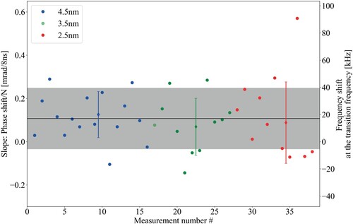
The phase measurements were carried out with a different (broader) pulse bandwidth than the Ramsey-comb measurements. The reason is the lower spectral power of the fibre-based frequency comb we now employ. This in turn required the use of an image intensifier (the 'Cricket' by Photonis), which reduced the resolution of our spectrometer. As a result, the same amount of spectral fringes has to be generated over a broader wavelength range. Most phase measurements were therefore done with a bandwidth of 4 nm (compared to 0.18 nm during the Ramsey-comb measurements), by opening the slit in the stretcher. The power of the 4 nm bandwidth beam, used as seed for the OPA during the phase measurements, was decreased to fit the power spectral density used for the RC measurements at 0.18 nm bandwidth. This was done in order to reproduce similar conditions in the OPA as during the RC measurements. In [38], it was shown that the measured phase shift with respect to the interpulse delay does not vary for different bandwidths (spanning 0.4 nm to 3 nm) with an accuracy of 9 mrad. In Figure A1, a comparison for the present system is shown of the detected linear phase shift slope at different bandwidths. At the transition frequency, this leads to a frequency correction according to Equation 4(A1) $\mathrm{\Delta }f=\left(8\mathrm{\Delta }\varphi \right)/\left(2\pi \mathrm{\Delta }N{T}_{rep}\right).$(A1) that is 20(17) kHz for 4.5 nm bandwidth, 11(21) kHz for 3.5 nm, and 14(30) kHz for 2.5 nm. The uncertainty of the measured frequency shift increases for smaller bandwidths. The reason is that for a smaller bandwidth, a higher resolution is required to observe a similar amount of interference fringes for an accurate determination. However, the optics and the Cricket image intensifier limit the resolution in this case. A phase shift between the pulses arises mostly from the interplay between a residual phase mismatch in the OPA and the amplification conditions [37]. It is important to realize that we are only sensitive to a change in phase shift between the two pulses. Although this shift depends strongly on alignment, there is very little dependence on wavelength, especially because the bandwidth we use is much smaller than the phase-matching bandwidth of the OPA crystals. The simulations performed in [37] show that theoretically no significant dependence of the measured phase shift on bandwidth is expected. This is confirmed by our measurements at 2.5 nm and 4.5 nm. Therefore we take the phase shift measurements performed at these bandwidths to be representative too for a bandwidth of 0.2 nm.

Figure A1. Comparison of the linear relative phase shifts for different bandwidths of the amplified FC laser. The average of all measurements is shown as the horizontal black line and its standard deviation by the grey band. The individual averages and standard deviations for each probed bandwidth are shown in the respective colour. No significant difference in the spread of slopes could be observed for bandwidths ranging between 2.5 and 4.5 nm.

Appendix 3: Improvements to the D₂ molecular beam apparatus

The molecular beam apparatus has been improved since the last Ramsey-comb measurements in H₂ [21], leading to a higher molecular density for a liquid-nitrogen-cooled beam, and a reduction of the beam divergence. The most important change has been the use of a pulsed valve developed in the group of F. Merkt at the ETH Zürich, as described in the main text. We describe below the other improvements we have made to the molecular beam apparatus.

The molecular beam path has been extended to reduce skimmer clogging and to optimize the density and collimation of the D₂ molecules in the interaction zone, as shown in Figure 8. A first skimmer (Sk1) of 8 mm diameter is placed 31 cm after the valve nozzle, while a second skimmer (Sk2) with a diameter of 3 mm is placed 82 cm after the nozzle. Both the source chamber with Sk1 and the intermediate chamber with Sk2 are independently pumped by a 500 l/s turbo-drag pump. The interaction zone is defined by the geometry of those skimmers, at 1.04 m from the valve nozzle, leading to a molecular beam diameter of about 3.8 mm where the excitation pulses meet. The valve is operated with a backing pressure of 1 bar of D₂ gas. Due to the finite bandwidth of the excitation laser in combination with a possible small misalignment of the two counterpropagating beams, the RC measurements are not completely first-order Doppler-free. To determine the first-order Doppler-free transition frequency, we vary the D₂ velocity by using either pure D₂ (at 999 m/s) or a mixture of 2 parts of D₂ mixed with 3 parts Ne. In the mixture collisions between D₂ and Ne slows down the D₂ molecules by a factor of 2 (571 m/s), but at the cost of a lower D₂ density. Moreover, the D₂ molecules are pushed out of the centre by the collisions with the heavier Ne atoms, resulting in an 80% loss of signal strength (when compared to pure D₂).

Appendix 4: Data taking procedure

Each Ramsey-comb measurement consists of three Ramsey fringes, at an interpulse delay corresponding to N = 3, 24 and 45. Every Ramsey fringe is obtained by scanning the pulse delay over 500 as in 8 steps (micro-delay steps). The micro-delay $\delta t$ and interpulse delay N were scanned randomly to collect 400 points for the measurement of three Ramsey fringes, resulting in a measurement time of 5 minutes and 43 seconds. In the analysis, the first 40 points, corresponding to 1.4 s, are discarded. This is done to take into account the settling time of the laser (especially the pulse energy) to the new settings of N and the repetition rate of the FC laser for each data point. Random scanning is made possible by pre-calibrating the feedback on the ratio and amplitude of the pulses. This is especially important for the large interpulse delay jumps used in the RC measurements as the final Nd:YAG amplifier of the pump laser system has a decreased gain for longer interpulse delays. The random scanning and short measuring time reduce the effect of drift effects on the extracted transition frequency.

References

- F. Biraben, Eur. Phys. J. Spec. Top. 172 (1), 109–119 (2009). doi:10.1140/epjst/e2009-01045-3
- C.G. Parthey, A. Matveev, J. Alnis, B. Bernhardt, A. Beyer, R. Holzwarth, A. Maistrou, R. Pohl, K. Predehl, T. Udem, T. Wilken, N. Kolachevsky, M. Abgrall, D. Rovera, C. Salomon, P. Laurent and T.W. Hänsch, Phys. Rev. Lett. 107 (20), 203001 (2011). doi:10.1103/PhysRevLett.107.203001
- R. Pohl, A. Antognini, F. Nez, F.D. Amaro, F. Biraben, J.M.R. Cardoso, D.S. Covita, A. Dax, S. Dhawan, L.M.P. Fernandes, A. Giesen, T. Graf, T.W. Hänsch, P. Indelicato, L. Julien, C.Y. Kao, P. Knowles, E.O. Le Bigot, Y.W. Liu, J.A.M. Lopes, L. Ludhova, C.M.B. Monteiro, F. Mulhauser, T. Nebel, P. Rabinowitz, J.M.F. dos Santos, L.A. Schaller, K. Schuhmann, C. Schwob, D. Taqqu, J.F.C.A. Veloso and F. Kottmann, Nature 466 (7303), 213–216 (2010). doi:10.1038/nature09250
- R. Pohl, R. Gilman, G.A. Miller and K. Pachucki, Annu. Rev. Nucl. Part. Sci. 63 (1), 175–204 (2013). doi:10.1146/nucl.2013.63.issue-1
- A. Beyer, L. Maisenbacher, A. Matveev, R. Pohl, K. Khabarova, A. Grinin, T. Lamour, D.C. Yost, T.W. Hänsch, N. Kolachevsky and T. Udem, Science 358 (6359), 79–85 (2017). doi:10.1126/science.aah6677
- N. Bezginov, T. Valdez, M. Horbatsch, A. Marsman, A.C. Vutha and E.A. Hessels, Science 365 (6457), 1007–1012 (2019). doi:10.1126/science.aau7807
- H. Fleurbaey, S. Galtier, S. Thomas, M. Bonnaud, L. Julien, F. Biraben, F. Nez, M. Abgrall and J. Guéna, Phys. Rev. Lett. 120 (18), 183001 (2018). doi:10.1103/PhysRevLett.120.183001
- A.D. Brandt, S.F. Cooper, C. Rasor, Z. Burkley, A. Matveev and D.C. Yost, Phys. Rev. Lett. 128 (2), 023001 (2022). doi:10.1103/PhysRevLett.128.023001
- R. Pohl, F. Nez, L.M.P. Fernandes, F.D. Amaro, F. Biraben, J.M.R. Cardoso, D.S. Covita, A. Dax, S. Dhawan, M. Diepold, A. Giesen, A.L. Gouvea, T. Graf, T.W. Hänsch, P. Indelicato, L. Julien, P. Knowles, F. Kottmann, E.L. Bigot, Y.W. Liu, J.A.M. Lopes, L. Ludhova, C.M.B. Monteiro, F. Mulhauser, T. Nebel, P. Rabinowitz, J.M.F.d. Santos, L.A. Schaller, K. Schuhmann, C. Schwob, D. Taqqu, J.F.C.A. Veloso and A. Antognini, T.C. Collaboration, Science 353 (6300), 669–673 (2016). doi:10.1126/science.aaf2468
- S. Patra, M. Germann, J.P. Karr, M. Haidar, L. Hilico, V.I. Korobov, F.M.J. Cozijn, K.S.E. Eikema, W. Ubachs and J.C.J. Koelemeij, Science 369 (6508), 1238–1241 (2020). doi:10.1126/science.aba0453
- S. Alighanbari, G.S. Giri, F.L. Constantin, V.I. Korobov and S. Schiller, Nature 581 (7807), 152–158 (2020). doi:10.1038/s41586-020-2261-5
- N. Hölsch, M. Beyer, E.J. Salumbides, K.S.E. Eikema, W. Ubachs, C. Jungen and F. Merkt, Phys. Rev. Lett. 122 (10), 103002 (2019). doi:10.1103/PhysRevLett.122.103002
- J. Hussels, N. Hölsch, C.F. Cheng, E.J. Salumbides, H.L. Bethlem, K.S.E. Eikema, C. Jungen, M. Beyer, F. Merkt and W. Ubachs, Phys. Rev. A. 105 (2), 022820 (2022). doi:10.1103/PhysRevA.105.022820
- M. Puchalski, J. Komasa, P. Czachorowski and K. Pachucki, Phys. Rev. Lett.122 (10), 103003 (2019). doi:10.1103/PhysRevLett.122.103003
- M. Siłkowski and K. Pachucki, Mol. Phys. 120 (19), e2062471 (2022). doi:10.1080/00268976.2022.2062471
- M. Puchalski, J. Komasa, A. Spyszkiewicz and K. Pachucki, Phys. Rev. A. 100 (2), 020503 (2019). doi:10.1103/PhysRevA.100.020503
- M. Beyer, N. Hölsch, J. Hussels, C.F. Cheng, E.J. Salumbides, K.S.E. Eikema, W. Ubachs, C. Jungen and F. Merkt, Phys. Rev. Lett. 123 (16), 163002 (2019). doi:10.1103/PhysRevLett.123.163002
- F.M.J. Cozijn, M.L. Diouf and W. Ubachs, Eur. Phys. J. D 76 (11), 220 (2022). doi:10.1140/epjd/s10053-022-00552-x
- J. Liu, D. Sprecher, C. Jungen, W. Ubachs and F. Merkt, J. Chem. Phys. 132 (15), 154301 (2010). doi:10.1063/1.3374426
- J. Liu, E. Salumbides, U. Hollenstein, J. Koelemeij, K. Eikema, W. Ubachs and F. Merkt, J. Chem. Phys. 130 (17), 174306 (2009). doi:10.1063/1.3120443
- R.K. Altmann, L.S. Dreissen, E.J. Salumbides, W. Ubachs and K.S.E. Eikema, Phys. Rev. Lett. 120 (4), 043204 (2018). doi:10.1103/PhysRevLett.120.043204
- V.A. Yerokhin, K. Pachucki and V. Patkóš, Ann. Phys. 531 (5), 1800324 (2019). doi:10.1002/andp.v531.5
- V.I. Korobov, L. Hilico and J.P. Karr, Phys. Rev. Lett. 118 (23), 233001 (2017). doi:10.1103/PhysRevLett.118.233001
- S. Hannemann, E.J. Salumbides, S. Witte, R.T. Zinkstok, E.J. van Duijn, K.S.E. Eikema and W. Ubachs, Phys. Rev. A. 74 (6), 062514 (2006). doi:10.1103/PhysRevA.74.062514
- J. Morgenweg, I. Barmes and K.S.E. Eikema, Nat. Phys. 10 (1), 30–33 (2014). doi:10.1038/nphys2807
- J. Morgenweg and K.S.E. Eikema, Phys. Rev. A. 89 (5), 052510 (2014). doi:10.1103/PhysRevA.89.052510
- N.F. Ramsey, Phys. Rev. 76 (7), 996–996 (1949). doi:10.1103/PhysRev.76.996
- N.F. Ramsey, Phys. Rev. 78 (6), 695–699 (1950). doi:10.1103/PhysRev.78.695
- R.K. Altmann, S. Galtier, L.S. Dreissen and K.S.E. Eikema, Phys. Rev. Lett.117 (17), 173201 (2016). doi:10.1103/PhysRevLett.117.173201
- L.S. Dreissen, C. Roth, E. Gründeman, J.J. Krauth, M. Favier and K.S.E. Eikema, Phys. Rev. Lett. 123 (14), 143001 (2019). doi:10.1103/PhysRevLett.123.143001
- L.S. Dreissen, C. Roth, E.L. Gründeman, J.J. Krauth, M.G.J. Favier and K.S.E. Eikema, Phys. Rev. A. 101 (5), 052509 (2020). doi:10.1103/PhysRevA.101.052509
- S. Hannemann, E.J. Salumbides and W. Ubachs, Opt. Lett. 32 (11), 1381 (2007). doi:10.1364/OL.32.001381
- H. Jóźwiak, H. Cybulski and P. Wcisło, J. Quant. Spectrosc. Radiat. Transf. 253, 107186 (2020). doi:10.1016/j.jqsrt.2020.107186
- N. Hölsch, I. Doran, M. Beyer and F. Merkt, J. Mol. Spectrosc.387, 111648 (2022). doi:10.1016/j.jms.2022.111648
- E. Tiesinga, P.J. Mohr, D.B. Newell and B.N. Taylor, J. Phys. Chem. Ref. Data 50 (3), 033105 (2021). doi:10.1063/5.0064853
- J. Morgenweg and K.S.E. Eikema, Laser. Phys. Lett. 9 (11), 781 (2012). doi:10.7452/lapl.201210079
- J. Morgenweg and K.S.E. Eikema, Opt. Express. 21 (5), 5275–5286 (2013). doi:10.1364/OE.21.005275
- R.K. Altmann, Ph. D. thesis, Vrije Universiteit Amsterdam, 2018.