Experiments in the Wild: Introducing the Within-Person Encouragement Design

Abstract

The within-person encouragement design introduced here combines methodological approaches from three research traditions: (a) the analysis of within-person couplings using multilevel models, (b) the experimental manipulation of a treatment variable at the within-person level, and (c) the use of random encouragements as instrumental variables to induce exogenous experimental variation when strict treatment adherence is unrealistic. The proposed combination of these approaches opens up new possibilities to study treatment effects of a broad range of behavioral variables in realistic everyday contexts. We introduce this new research design together with a corresponding data analysis framework: instrumental variable estimation with two-level structural equation models. Using simulations, we show that the approach is applicable with feasible design dimensions regarding numbers of measurement occasions and participants and realistic assumptions about adherence to the encouragement conditions. Possible applications and extensions, as well as potential problems and limitations are discussed.

Keywords:

• Experimental manipulation
• within-person design
• encouragement design
• instrumental variable estimation
• multilevel modeling
• ambulatory assessment

Introduction

In this paper, we propose a new study design and a corresponding data-analysis framework. The proposed design brings together three methodological approaches to study human behavior, from three different research traditions: (a) the analysis of within-person couplings using multilevel models – from research using intensive longitudinal data to study within-person processes and individual differences therein, (b) the experimental manipulation of a treatment variable at the within-person level – from research using single-case designs to evaluate causal effects, and (c) the use of encouragement designs – from research evaluating treatment effects when strict treatment adherence is unrealistic. The proposed combination of these approaches – the within-person encouragement design – opens up new possibilities to study (individual differences in) treatment effects of a broad range of behavioral variables in realistic everyday contexts (i.e., in the wild). We introduce this new design by first describing benefits and limitations of each of the existing traditions, and then show how they can be combined in a way that brings together their strengths and overcomes their limitations. As a corresponding data-analysis framework, we propose instrumental variable estimation implemented in a two-level structural equation model. Based on simulation studies, we show that this allows conducting within-person encouragement studies with feasible design dimensions regarding number of participants and measurement occasions and with realistic assumptions about treatment adherence. In combination, the within-person encouragement design and two-level instrumental variable estimation provide a powerful and flexible approach to investigate experimental effects – and individual differences therein – at the within-person level in many settings where strict manipulation of behavior is unrealistic or impossible.

Within-person couplings in intensive longitudinal designs

In psychology, we can witness a growing interest in the investigation of within-person processes in everyday life (Mehl & Conner, 2012) using intensive longitudinal methods (Bolger & Laurenceau, 2013). These have been introduced in psychological research using various terminology, including diary methods (Bolger, Davis & Rafaeli, 2003), experience sampling methods (Hektner, Schmidt, & Csikszentmihalyi, 2007), ecological momentary assessment (Shiffman, Stone, & Hufford, 2008), or ambulatory assessment (Trull & Ebner-Priemer, 2013). In addition to aiming at increased ecological validity, at objective assessments of behavior, and at more valid self-reports, the increasing interest in intensive longitudinal methods is fueled by the acknowledgement that relations of variables within persons over time can differ across people as well as from the relations observable at the level of between-person differences (Hamaker, 2012; Molenaar, 2004). A growing number of studies use such designs and show average couplings (i.e., fixed effects of the intraindividual regression) of variables as well as individual differences (i.e., corresponding random effects) in the strength of within-person couplings across occasions. Those can be couplings between variables such as intrusive thoughts and negative affect (Brose, Schmiedek, Lövdén, & Lindenberger, 2011), need fulfillment and mood (Neubauer, Lerche, & Voss, 2018), snack craving and snack consumption (Richard, Meule, Reichenberger, & Blechert, 2017), or stressful events and cognition (Sliwinski, Smyth, Hofer, & Stawski, 2006). Significant random effects of such couplings indicate that people function differently and thereby can hint at the possibility that also interventions might be differently effective for different people. Take for example the within-person coupling of sleep quality and cognitive performance in elementary school children reported by Könen, Dirk, and Schmiedek (2015). The fixed effect of this coupling indicates that, on average, days with better self-reported sleep quality tend to be days with better cognitive performance. This effect is associated with a significant random effect, however, that implies individual deviations from the average strength of this coupling. That is, the importance of sleep quality for cognition varies across children. Such information could be used to tailor interventions to empirically determined individual characteristics – like trying to improve sleep quality for children who show particularly strong couplings with cognition. Before doing so, however, it needs to be established that the correlational evidence provided by the observed coupling is produced by the supposed causal mechanism, that is, that the coupling is due to sleep quality causally influencing cognitive performance (rather than a third variable affecting both sleep quality and cognitive performance). What is needed to demonstrate causal relations at the within-person level is experimental evidence based on controlled variation (ideally, in a randomized fashion) of the supposed antecedent within persons over time.

In sum, the investigation of naturally occurring within-person couplings can be a good starting point to identify associations among variables that are potentially causal, with potentially varying degrees of strength of the causal relation between persons. The established multilevel analysis framework offers great flexibility to investigate the associated fixed and random effects. The observational nature of the results from typical studies, however, prevents causal inference and calls for (the addition of) experimental approaches.

Within-person experimental manipulations

Experimental within-person manipulations are well established in general psychology and also have a long tradition in clinical psychology (Morgan & Morgan, 2001), medicine (Kravitz, Duan, & the DEcIDE Methods Center N-of-1 Guidance Panel, 2014), and educational psychology (Phye, Robinson, & Levin, 2005). In general psychology, the use of within-subject factors mainly serves to increase statistical power by freeing residual variance from stable between-person differences and typically aims at identifying average causal effects for a sample of participants – and not the variation of effects across participants. In clinical psychology and medicine, and also in educational psychology (Schmitz, 2006), there is a rich tradition of “N-of-1 trials”, in which single participants are investigated under different conditions. For example, the effect of a drug is examined by comparing phases in which it is applied to phases in which a placebo is given. Such interrupted time series (Shadish, Cook, & Campbell, 2002), or ABA(B) designs have been proposed and used for decades and are receiving growing interest in the advent of patient-centered approaches (Schork, 2015). When applied to samples of participants, such designs can be analyzed flexibly using multilevel modeling approaches (see Lischetzke, Reis, & Arndt, 2015; Shadish, Kyse, & Rindskopf, 2013).

There are reasons for also considering experimental manipulations that change between treatment and control conditions with a higher frequency, in analogy to block- versus trial-based sequences in general psychology. First, the comparison of longer phases of treatment and control conditions is more likely to be confounded with period or maturation effects. Second, for certain behaviors, it is realistic to assume relatively immediate and short-lived effects, while it also may be unrealistic to expect the behavior to be shown consistently over extended periods of time. The effect of a good night’s sleep on affect, for example, likely has the duration of a whole day at maximum. At the same time, it might be difficult to ensure that participants show a particular sleep behavior consistently over a period of several weeks.

There are many examples of behaviors of this kind that might have beneficial effects on health, mood, cognition, and performance. Those include, for example, sleep, physical activity, relaxation techniques, and nutrition. In a fascinating series of studies with self-experimentation, Seth Roberts (2004) investigated cause-effect relations for himself by manipulating very specific behaviors – like seeing faces on television, standing for 8 hours per day, and eating sushi – on the basis of (clusters of) days, which allowed him to derive hypotheses about causal mechanisms that benefit psychological and physiological well-being. This is a basic feature of the study design that we want to introduce here: the random manipulation of a treatment across occasions. That is, a certain behavior, like going to bed early, having a run, or eating a particular diet for breakfast, that is thought to have an immediate effect (operationally: before the next occasions) on an outcome, is “turned on” on a random subsample of occasions on which it could be shown in principle and “turned off” on the remaining occasions.

In health psychology, there have been recent developments to support health-beneficial behavior that could similarly be turned on and off in situations of opportunity or vulnerability, using so-called just-in-time adaptive interventions (Klasnja et al., 2015). Based on a “micro-randomization” of prompts to show a certain behavior, like being physically active, at corresponding decision points in people’s daily lives, the causal effect of such prompts on actual behavior (e.g., step count) can be estimated (Klasnja et al., 2015). Our within-person encouragement approach presented here can be viewed as an extension of this work, in that it also allows to estimate the causal effect of, for example, a health behavior (e.g., physical activity) on further outcome variables (e.g., momentary positive affect). In this way, what is considered the intervention (e.g., a prompt to be physically active) and outcome (e.g., step count) by Klasnja et al. (2015) is termed encouragement and treatment in our approach, while what we term outcome is a further variable (e.g., positive affect) that is considered to be causally influenced by the treatment.

This extension is based on the acknowledgement of the substantial practical limitation that, in their everyday lives, people will often be unlikely to show perfect adherence to (randomized) prompts. Neither will it be possible for participants to show a certain behavior every time it is requested by prompts based on a random sequence, nor will people always be willing not to show a behavior because the random sequence dictates them so. Even if people generally commit to participate in a study which puts, for example, physical exercise under experimental control, they might not be willing or able to go for a run on each particular day a smartphone-based study application tells them to do so. Conversely, they might want to take the opportunity to run on a day when the weather is particularly inviting, even if there has been no prompt by the application. Hence, practical and ethical considerations will often render full adherence unlikely and thereby threaten the integrity of the experimental manipulation. The solution we are proposing to this is borrowed from so-called encouragement designs that have been established by educational scientists for situations in which also practical or ethical constraints prohibit strict manipulation.

Encouragement designs and instrumental variable estimation

Instead of randomizing participants directly into treatment and control conditions of a certain intervention, in encouragement designs, the randomization is done into groups that are either encouraged, or not, to participate (Bradlow, 1998; Powers & Swinton, 1984). This can be done, for example, by providing information on the benefits of the intervention or by giving out vouchers that allow taking the treatment. A first example in the literature was the evaluation of the educational TV series Sesame Street, in which information about the program’s benefits and encouragement to let children watch it was provided to a random subset of participating families (Ball & Bogatz, 1970, 1971).

A straightforward way of analyzing data from a study with an encouragement design is to use an intention-to-treat analysis. In an intention-to-treat analysis, the encouraged group is directly compared to the not-encouraged group. Given randomization into these two conditions, the causal interpretation of the resulting effect estimate is ensured – irrespective of whether or not participants finally took the treatment. However, the resulting effect estimate consequently provides an estimate of the effect of being encouraged – and not an estimate of the effect of the treatment itself. The effect of the treatment in an encouragement design can be estimated using instrumental variable estimation (IVE) techniques (Angrist, Imbens, & Rubin, 1996). In these, the encouragement is used as an instrumental variable, which allows investigating causal effects of the treatment on the outcome even if adherence is not perfect – provided that two conditions are met. The first condition is empirically testable and requires that there is a correlation of the randomized encouragement and the treatment. That is, there must be a systematic and reliable effect (the stronger the better) of the encouragement (i.e., the instrumental variable) on the treatment behavior: people should be more likely to show the behavior when encouraged than when not. The second condition is not directly testable and can only be argued for on theoretical grounds. It includes the assumption that any effect of the encouragement on the outcome is fully mediated through the treatment, that is, there must not be any direct or otherwise mediated effects of the encouragement. Provided that the two conditions are met, IVE can be conducted with two-stage least squares (2SLS) or its path-analytic equivalent. Other than two-step approaches in which (a), in a first regression, the treatment variable is regressed on the instrument, (b), in a second regression, the outcome variable is then regressed on the predicted values from the first regression, 2SLS and their path-analytic counterparts directly provide correct standard errors. Furthermore, IVE provides a consistent estimate of the so-called local average treatment effect (LATE; Angrist et al., 1996). In between-person designs, the LATE is the effect of the treatment for the (theoretical) population of participants who would be complying with the encouragement, by showing the corresponding behavior when encouraged to do so, and not showing it when no encouragement is provided.

The main idea behind the present work is to transfer such encouragement designs and the associated IVE techniques from the between-person to the within-person level. This opens the possibility to investigate causal effects of everyday behaviors, and individual differences therein, under ecologically valid conditions. The proposed approach can augment previous studies that have already used parts of the components of a within-person encouragement study. For example, in a study by Klasnja et al. (2019) participants received randomized prompts to increase physical activity (vs. decrease sedentary behavior or no encouragement) in their daily lives. Physical activity was obtained as step counts within 30 minutes following the prompt. In this study, the randomized prompts correspond to the encouragement in our terminology, and the step count is the treatment behavior. Additionally assessing a theoretically relevant outcome (e.g., affect 30 minutes after the prompt) would yield a full within-person encouragement design as proposed here. Similarly, encouragements could be added to observational studies conducted in daily life. For example, hobby musicians’ positive affect was reported to be higher on days when they engaged in music making (vs. not; Koehler & Neubauer, 2019). Here, music making is the behavior and positive affect is the outcome. An encouragement could be added to this study, encouraging participants in the morning to engage in music making today (vs. not) in a randomized fashion, and examine the effect of the experimentally induced variance of self-reported music making on the outcome (positive affect).

In the following, we will provide (a) the general procedure of planning and conducting a study with a within-person encouragement design, (b) details on how data from such a study can be analyzed with two-level structural equation modeling, and (c) two simulation studies that examine the power to detect causal effects under varying design dimensions (i.e., number of participants and measurement occasions) and different strength of the encouragement adherence and treatment effects. Finally, potential problems, limitations, and possible applications and extensions will be discussed.

Planning and conducting a study with a within-person encouragement design

The steps of planning and conducting a study with a within-person encouragement design partly have characteristics that deviate from other existing research designs and will therefore be outlined in some detail here. Those include the definition of outcome and treatment, the negotiation of feasible intervention regimes, and the implementation of the intervention.

Step 1. Define outcome and target population. The first step is to define an outcome variable of the purposed intervention. This could be any variable that shows temporal variation within persons of a (also to-be-defined) target population. For example, psychological well-being, cognitive performance, or aspects of physical health could be such outcomes. Preferably, it should be possible to assess the outcome in an online manner in peoples’ everyday lives. This includes objective measures (e.g., actigraphy, physiological markers) and/or self-report ratings, which can be assessed repeatedly using experience-sampling techniques. Alternatively, some outcome measures may also be assessed in repeatedly visited laboratory settings, or retrospectively, for example, via end-of-day diaries. Besides evidence of the validity of these outcome measures, it needs to be ensured that they are able to reliably capture within-person changes (Cranford, Shrout, Iida, Rafaeli, Yip, & Bolger, 2006; Geldhof, Preacher, & Zyphur, 2014). If the measures show little sensitivity to within-person changes, this reduces the power to be able to detect causal within-person relations.

Step 2. Define a treatment behavior and the population of situations in which it can be shown. The next step is to identify the behavior to be manipulated by encouragements. This ought to be a behavior that (a) is thought to have a causal effect on the outcome, (b) is under the participants' control (at least for certain periods of time), and (c) can potentially be shown on a large enough number of occasions. Regarding the assumption of a causal effect, the researcher can draw on theoretical considerations supporting a causal mechanism that links the treatment behavior to the outcome, as well as on empirical evidence demonstrating, or at least suggesting, such causal influences. Similarly to the conditions that must be fulfilled for the outcome, the treatment behavior needs to show within-person variation that can be assessed with sufficient reliability using objective measures and/or self-report ratings.

Regarding participants’ control of the behavior, it needs to be ensured that participants are free in their choice and ability to show – or not to show – the behavior at a to-be-defined population of situations, which ideally should be large. Exemplary cases are all kinds of daily routines, like eating/drinking, getting to work, or spending leisure time, that can be implemented in different ways (e.g., having a coffee for breakfast or not, taking the bike to get to work or not, doing yoga during leisure time or not).

Step 3. Recruit participants and negotiate intervention regime. While an encouragement design in principle could be implemented as a single-case study (see Discussion), the power to detect an average effect and the possibility to investigate individual differences in the strength of the effect hinges on conducting studies with a sample of participants. It is therefore necessary to find enough participants who are willing to put a certain behavior under experimental control for a period of time. For a sample of participants who are generally willing to participate in the study, it may be further necessary to negotiate individually the details of the treatment regime. This includes agreement on a specific definition of the behavior (e.g., running at a certain pace for a certain minimum amount of time), on a study period (e.g., four weeks), and on a set of situations within the study period. The latter could be longer time frames (e.g., weekend days, on which the behavior can be shown at any deliberate time) as well as more circumscribed situations (e.g., the time being in bed before trying to fall asleep).

Participants should agree to (a) try to show the behavior when prompted and report on whether they did so (if not objectively measured) and (b) not to show the behavior when not prompted and report any behavior that has been shown nonetheless. The second requirement can be relaxed by defining a set of situations in which the behavior is shown independently of the study (e.g., participating in a walking group each Sunday morning), and then not considering these occasions in the analyses. For ethical reasons, participants need to be informed that they are free to not adhere to the encouragements to any degree, but that the pursuit of the study aims generally hinges on a high level of adherence.

Ideally, a set of situations (e.g., weekday mornings) within a certain period of time (e.g., 10 weeks) can be picked, on which the treatment behavior (e.g., taking the bike instead of the car to get to work) could be shown equally well. In this case, encouragements could be given on random subset of 50% of all the possible situations, providing an optimal base rate and ensuring a high compliance rate of the actual treatment behavior. Practical as well as ethical constraints, however, may force deviations from such an optimal situation. For example, if a participant wants to show the treatment behavior not more often than on 25% of the total set of situations, it may be better to use a 25% encouragement rate on this total set than agreeing on a reduced set of situations, to which again a 50% encouragement rate could be applied, for the intervention. Creating an optimal individual design in the first place will require to ensure that the participant is not suffering any financial, social, health-related, or psychological disadvantages, while also trying to balance practical constraints and aspects of statistical power.

Step 4. Implement the intervention. Implementation of the treatment requires providing participants with encouragements at a random subset of the situations determined in Step 3. While the way encouragements are provided to participants could also draw on “analog” media – like envelopes with enclosed instructions for each day, or daily phone calls by research assistants – applications on modern smartphones provide the most flexible and reliable means to prompt participants directly in their daily lives and right at some optimal time point (e.g., half an hour before a specified occasion). Technically, it is straightforward to adapt existing software for smartphone-based experience-sampling studies with time-based designs (Bolger et al., 2003) to provide the encouragements. A great advantage of using smartphone-based provision of encouragements is that for many applications this will allow to also collect objective information on treatment implementation (e.g., recording of physical activity after an encouragement to go for a run) as well as immediate measurements of the outcome variable (e.g., cognitive performance or self-reports of affect). Both kinds of information are essential for the final step of analyzing the data.

Analyzing data with two-level structural equation models

An established approach to analyze data from encouragement designs, or experiments with “fuzzy” assignment to treatment in general, is IVE with two-stage least squares (2SLS) estimation. Modern day applications of this approach provide for the simultaneous estimation of two regression models, with the first one predicting the treatment variable with the instrument (here: the encouragement), and the second one using predicted treatment values from the first stage as predictor of the outcome. Under the exclusion assumption of no association of the instrument with the outcome other than through the treatment, this second regression of the 2SLS procedure provides a consistent estimate of the causal effect of the treatment on the outcome. This is possible, because the first step “extracts” the part of variation in the treatment that is due to the randomized encouragement and can therefore be considered exogenous. Restraining the effect of the treatment on the outcome to this part of treatment variation provides an estimate of the treatment effect (TE).

As a data-analytical alternative that provides equivalent results, one can also employ path analysis using structural equation modeling (SEM) and maximum likelihood estimation (see Bollen, 2012, for a review). Here, direct paths from the instrument to the treatment and from the treatment to the outcome are estimated while no path from instrument to outcome is specified. Importantly, the residual terms of the treatment and the outcome need to be allowed to correlate with each other. The correlation of these residual terms captures all other (and potentially endogenous) shared influences of the treatment and the outcome, apart from the influence of the encouragement. If, for example, participants tend to go for a run (i.e., the treatment) on days when the sun is shining, irrespective of whether an encouragement is provided or not, and sunshine also positively influences mood (i.e., the outcome), this shared influence would be caught by the correlation of the residuals.

If we were to analyze data from a within-person encouragement study with one single participant, we could draw on either one of these existing approaches to estimate the causal effect of the encouraged treatment. Regarding the more general case of a study with a sample of participants, a natural data-analytic approach is to combine their data and use multilevel modeling for repeated observations (Level 1) within subjects (Level 2). Such a multilevel approach comes with the advantage of increasing the power to detect average treatment effects by combining the data from several participants, while allowing to also investigate individual differences in the strength of the treatment effect by including random effects at Level 2. The path-analytical approach to IVE can be implemented in a multilevel model by drawing on the possibilities provided by multilevel structural equation modeling (Muthén, 1994; Skrondal & Rabe-Hesketh, 2004), which allows to implement the path model for IVE estimation at Level 1 and to include random effects regarding its parameters at Level 2. Figure 1 illustrates this model, which will be explained in detail next.

Figure 1. Graphical representation of the two-level SEM for path-analytic IVE. On Level 1, of repeated occasions within persons, the path model with direct effects of the observed instrument (i.e., the encouragement condition) on the observed treatment variable (i.e., the targeted behavior) and of the treatment on the observed outcome variable is specified, together with the variances and the covariance (σ²_T, σ²_O, and ψ_TO) of the residual terms of the treatment (e_T) and the outcome (e_O) at the within-person level. On Level 2 (between-person differences), the fixed effects of the encouragement on the treatment (β_ET) and of the treatment on the outcome (β_TO), as well as fixed intercepts of the treatment (β_Int(T)) and the outcome (β_Int(O)) are modeled (indicated as paths from the triangle, with represents a constant). Also, random effects (i.e., between-person differences) of these effects (σ²_ET and σ²_TO) and of the intercepts (σ²_Int(T) and σ²_Int(O)), as well as their covariances (double-headed arrows; parameters not shown) are included.

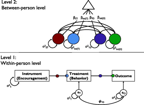
Level 1 path model. The path-analytic approach to IVE requires a mediation path model with direct paths from instrument to treatment and from treatment to outcome, together with a covariance of the residual terms of treatment and outcome. In its basic form, this path model can easily be implemented in standard SEM software. Taking into account more complex time-related aspects, like autocorrelations of the variables across measurement occasions, requires extensions, like the use of dynamic SEM (Asparouhov, Hamaker, & Muthen, 2018), to be introduced later.

Level 2 random effects. In a two-level SEM, the Level 1 parameters can potentially vary across the units of Level 2. In our application, this leads to the possibility to not only estimate fixed (average), but also random effects, for the intercept and regression path parameters. Specifically, one can regard individual differences in the intercepts of the treatment and outcome variable, as well as individual differences in the strength of the paths from encouragement to treatment and from treatment to outcome. Regarding the intercepts, participants might differ in their baseline frequency or intensity of the treatment behavior when no encouragements are provided and in their baseline level of the outcome in the absence of the treatment behavior. Regarding the regression paths, participants might differ in their propensity to show the treatment behavior given an encouragement and in their individual effectiveness of the treatment regarding the outcome (i.e., their individual treatment effects). All these individual differences can be of interest from a substantive point of view. Therefore, being able to test and estimate the size of the corresponding random variance parameters is a major advantage of the proposed approach. Furthermore, covariances of the random effects might be of interest. As just one example, researchers might want to know if participants who are more likely to follow the encouragements are also showing stronger effects of the treatment.

Finally, the Level 2 model could be extended to include other Level 2 variables, like person characteristics that are hypothesized to explain individual differences in treatment adherence or effectiveness. As known from the application of multilevel models, however, the inclusion of several random effects and their covariances is prone to quickly lead to estimation problems, like nonconvergence or improper solutions (i.e., nonpositive-definite covariance matrices of random effects or their Hessian). Therefore, the possibility to estimate all four random effects and their six covariances of the baseline model proposed here might be limited in practical applications. To investigate the practicality and the statistical properties (bias and power) of the proposed modeling approach under different sizes of the design dimensions (i.e., number of participants and number of occasions), different sizes of encouragement adherence and treatment effectiveness, and for different numbers of random effects being present, we conducted two simulation studies. Simulation 1 evaluated main effects of these design dimensions, as well as their interactions. Furthermore, it addressed the question of how the size of random effects (i.e., individual differences), and whether or not they are included in the model estimation, influences results. Simulation 2 focused on a subset of the conditions in Simulation 1 and investigated how the presence and size of autoregression in the treatment and outcome variables, and whether or not such autoregression is included in the model estimation, influences results.

Simulation study 1

Method

The overall population models simulated follow the depiction in Figure 1 (without the covariances of the random effects). In the present simulation, we manipulated the following parameters:

1. Adherence effect (AE; the within-person effect of encouragement on treatment behavior; ${\mathrm{\beta }}_{\mathrm{ET}}$ in Figure 1). As this parameter represents the central difference of the proposed approach to classic experimentation with perfect adherence, we covered the full range of very high (0.80) to very low (0.10) adherence rates.

2. Treatment effect (TE; the within-person effect of the treatment behavior on the outcome; ${\beta }_{\mathrm{TO}}$ in Figure 1). The proposed approach has a wide range of possible applications with treatments differing in expected effectiveness. We therefore varied treatment effect size from small to medium sized effects.

3. Covariance of the residuals of the behavior with the residuals of the outcome (representing any association of the treatment behavior with the outcome that is not due to the encouragement; ${\mathrm{\psi }}_{\mathrm{TO}}$ in Figure 1). In different possible applications, the number and strength of common or correlated influences on the treatment behavior and the outcome can vary widely. We therefore included different levels of residual correlation, ranging from zero to strong (0.60).

4. The number of study participants (N). Number of participants was varied from sample sizes that can be considered small (20) to large (100) for intensive longitudinal studies.

5. The number of measurement occasions per participant (T). Number of occasions was varied from sample sizes that can be considered small (20) to large (100) for intensive longitudinal studies.

6. The random variance of AE (i.e., the size of between-person differences in the adherence effect; ${\sigma }_{\mathrm{ET}}^2$ in Figure 1). Simulated variances ranged from small (10% of the smallest fixed AE), to large (50% of the largest fixed AE).

7. The random variance of TE (i.e., the size of between-person differences in the TE; ${\sigma }_{\mathrm{TO}}^2$in Figure 1). Simulated variances ranged from small (10% of the smallest fixed TE), to large (up to 50% of the largest fixed TE). We decided to use the same variances as for the random effect of the AE (excluding the largest variance that would have been larger than 50% of the largest fixed TE).

Specifically, encouragement was a dichotomous variable (i.e., encouragement on vs. off) with an equal distribution (i.e., encouragement was given at 50% of all measurements) while behavior and outcome were implemented as continuous, normally distributed variables. Level 1 residual variances of these two variables (${\sigma }_{\mathrm{T}}^2$ and ${\mathrm{\sigma }}_{\mathrm{O}}^2$) were set to 1; accordingly, the size of the AE can be interpreted in terms of Cohen’s d (Cohen, 1988). Between-person variances of treatment and outcome (${\sigma }_{\mathrm{Int}\left(\mathrm{T}\right)}^2$ and ${\sigma }_{\mathrm{Int}\left(\mathrm{O}\right)}^2$) were also set to 1 in the population model; all between-person covariances (i.e., covariances among random intercepts and random slopes) were set to zero to keep the model parsimonious. Table 1 lists the conditions realized in the present simulation study. Crossing all factors listed in Table 1 results in a total of 21,600 cells. Note, however, that we removed conditions in which low fixed effects went along with high random variances. We chose such a partially crossed design for reasons of interpretability. For example, a fixed AE of 0.20 (i.e., a small effect of the encouragement on behavior) combined with a random slope variance of AE of 0.20 (corresponding to a standard deviation of 0.45) would indicate that for a large portion of study participants, the encouragement would have a negative effect on behavior (assuming a normal distribution of AE, for approximately 33% of the study participants the AE would be negative). Although such instances might be observed in empirical data, such cases would likely need to be interpreted as evidence against a general efficacy of the encouragement. For the present study, we included only those cells when the fixed effects were approximately as large as the random slope SD, yielding 9576 cells that were realized in the present study. For each cell, 1000 samples were simulated.

Table 1. Conditions realized in Simulation Study 1.

Factor	Levels
Adherence effect	0.1, 0.2, 0.3, 0.4, 0.5, 0.8
Treatment effect	0.1, 0.2, 0.3, 0.4, 0.5
Level 1 residual covariance	0, 0.2, 0.4, 0.6
Level 2 sample size (N)	20, 50, 100
Level 1 sample size (T)	20, 50, 100
Random variance (adherence effect)	0.01, 0.05^a, 0.1^b, 0.2^c, 0.4^d
Random variance (treatment effect)	0.01, 0.05^e, 0.1^f, 0.2^g

Note. 1000 repetitions were simulated for each cell of the design.

^aOnly included if adherence effect was at least 0.2.

^bOnly included if adherence effect was at least 0.3.

^cOnly included if adherence effect was at least 0.4.

^dOnly included if adherence effect was 0.8.

^eOnly included if treatment effect was at least 0.2.

^fOnly included if treatment effect was at least 0.3.

^gOnly included if treatment effect was at least 0.4.

The models were re-estimated in two conditions: Whereas in the first condition, random variances of the AE and the TE were estimated, these variances were constrained to zero in the second condition. This allowed us to examine the effect of false fixations of random variances on estimation performance (e.g., because of convergence problems or improper solutions when trying to estimate random effects). All models were estimated using the robust maximum likelihood estimator (MLR) Mplus Version 8 (Muthén & Muthén, 2017), as this is a likely choice in empirical applications where, other than in our simulation study, the fulfillment of distributional assumptions will often not be guaranteed. Data were generated using the Monte Carlo option of Mplus. Mplus code for the simulation in one exemplary cell is provided in the online supplemental material.

The main parameter of interest in our simulation study was the fixed TE (i.e., the average within-person effect of the treatment on the outcome). We examined relative bias of the TE (=difference of estimated TE and the population TE, divided by the population TE; result multiplied by 100) and power (=the proportion of repetitions, in which the p-value of the fixed treatment effect was less than 0.05) of this parameter as primary outcomes in this study. To investigate the precision in the estimation, we also examined the mean squared error (MSE; this parameter combines information on both bias and variability of the estimate) and the 95% coverage rate (=the proportion of repetitions in which the 95% confidence interval covers the true parameter) as secondary outcomes (results on MSE and 95% coverage rate are reported in the supplemental online material).

Results

In the first set of analyses, we investigated convergence rates, bias of the TE, and power to detect TE in the models in which the random variances of the AE and TE were freely estimated. We then compared the results to the ones obtained when these random slope variances were constrained to zero.

Unconstrained models. In most of the cells (7598; 79.3%), convergence errors occurred in less than 5% of the samples; in 6.2% of all cells (589), there were convergence errors for more than 25% of the samples. The vast majority of these cases included small sample size on Level 2 (N = 20; 87.4%), and/or small sample size on Level 1 (T = 20; 81.0%), and/or small population random variances of the AE (≤0.05; 94.4%), and/or TE (≤0.05; 77.9%).

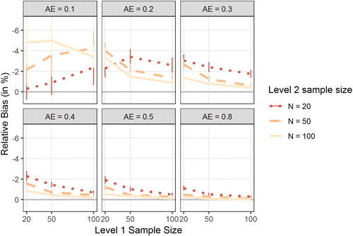
IVE is known to exhibit small sample bias in the estimates of treatment effects (see, e.g., Sawa, 1969). To determine the degree of this bias in the present study, we computed the relative bias in the estimation of the TE (negative scores indicate underestimation of the true effect). Figure 2 depicts the bias in the estimated TE as a function of T (x-axis), N (separate lines), and the size of the population AE (separate plots). Overall, results indicated only modest bias (5% or less). With moderate sample sizes on both Level 1 and Level 2 (T = 50 and N = 50), bias in TE was around 2% or less if the AE was 0.20 or higher. Overall, bias decreased with increasing sample size and increasing AE, but the results in the conditions with AE = 0.10 were at odds with this overall picture. Note, however, that there were markedly fewer data points in the AE = 0.10 condition because we realized only conditions with a random slope variance of 0.01 in these cells. Furthermore, these conditions were particularly affected by convergence errors.

Figure 2. Figure displays the relative bias in the estimation of the treatment effect (TE) in the unconstrained models as a function of Level 1 sample size (number of measurement occasions T; x-axis), Level 2 sample size (number of study participants N; separate lines), and the population adherence effect (AE; separate plots). Error bars indicate 95% confidence intervals. Note that the y-axis has been reverted.

To examine the power obtained for the TE in the simulated data sets, we predicted power (percentage of statistically significant, α < 0.05, TE estimates in each cell of the simulation design) by the main effects and two-way interactions of the seven factors that were varied in the present simulation study. In total, these seven predictors accounted for 91.0% of the variance in empirical power. Given the large sample size of 9,576, only effects that accounted for more than 0.5% of the variance (partial eta-squared; ${\eta }_{\mathrm{p}}^2$) were retained. Results can be found in Table 2.

Table 2. Factors associated with power for the treatment effect.

Effect	Effect size (${\eta }_{\mathrm{p}}^2$)
Level-2 sample size (N)	0.598
Level-1 sample size (T)	0.620
Adherence effect (AE)	0.758
Treatment effect (TE)	0.741
Adherence effect random variance (rvAE)	0.069
Treatment effect random variance (rvTE)	0.013
N × T	0.052
N × AE	0.198
N × TE	0.055
N × rvAE	0.008
N × rvTE	0.007
T × AE	0.235
T × TE	0.065
T × rvAE	0.006
AE × TE	0.137
AE × rvAE	0.031
TE × rvAE	0.006

Note. Only main effects and two-way interactions with ${\eta }_{\mathrm{p}}^2$ > 0.005 were retained. N = 9576; df_Residual = 9448.

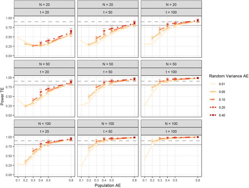
Not surprisingly, the population TE had a strong effect on the power for the TE. Level 2 sample size had roughly the same effect on power as Level 1 sample size. That is, increasing the number of study participants has a comparable effect on power as increasing the number of measurement occasions per participant. The AE also had a strong impact on power; in fact, the effect size was even slightly larger than the effect of population TE. To further illuminate the effects of the manipulated factors on power, Figure 3 shows power as a function of population AE, random variance in AE, N, and T. This figure shows that adequate power for the TE can be obtained in samples of moderate size (N = 50, T = 50) as long as the AE is of moderate size as well (0.50). Note that this combines all population TEs (from 0.1 to 0.5). Large values of the TE (0.40 or 0.50) can be detected with sufficient power even with smaller AE (see Figure S1 in the supplemental online material for power separated by population TE). It can also be seen from Figure 3 that power increases slightly with larger between-person differences in AE. Large between-person differences in the AE increase the amount of variance in the behavior that is caused by the encouragement, which in turn increases the power to detect the association between (experimentally induced) within-person variance in the behavior and the outcome. In a final set of analyses, we examined Type-I error when the true TE is zero. To that end, we simulated data with TE = 0 and ${\sigma }_{\mathrm{TO}}^2$ = 0.01 (the other conditions were the same as in the previous models). Across all conditions, alpha error for a true zero TE was 4.35% (95% CI: [4.23%; 4.47%]).

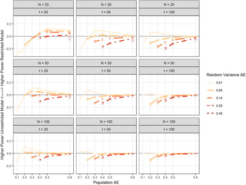
Figure 3. Figure depicts power of the treatment effect (TE) in the unconstrained models as a function of the population adherence effect (AE; x-axis), Level 2 sample size (number of study participants N; rows), Level 1 sample size (number of measurement occasions per participants T; columns), and the population random variance of the AE (Random Variance AE; separate lines). Error bars indicate 95% confidence intervals. Gray horizontal lines mark 80% power (solid line) and 90% power (dashed line).

Constrained models. Analyses were repeated for the same population models, but with the random slope variances constrained to zero in the estimated models. By this, we aimed at reducing the number of convergence errors (removing random variances in case of convergence errors is a solution often deployed by applied researchers). Results revealed better convergence rates compared to the unconstrained model: in 98.2% (9399) of the cells, convergence errors occurred in less than 5% of the samples (compared to 79.3% in the unconstrained models) and there was no cell with convergence errors in more than 25% of the samples (versus 589 such cells in the unconstrained models).

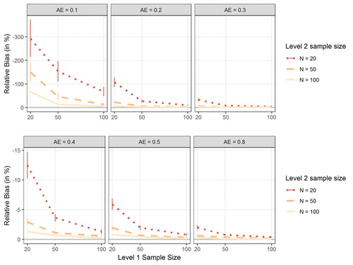
When examining the bias in the TE, the overall pattern was comparable to the pattern observed among the unconstrained models (see Figure 4): bias decreased with increasing N, increasing T, and increasing AE. Furthermore, bias was modest in conditions with moderate AE (.40 or higher) and moderate sample sizes on Level 1 and Level 2 (T = 50 and N = 50). Overall, however, bias was larger in the constrained than in the unconstrained models, in particular in small samples and with small AE. In the most unfavorable condition (N = 20, T = 20, AE = .10), relative bias in TE was −293% (note the altered range of the y-axis in Figure 4).

Figure 4. Figure shows the relative bias in the estimation of the treatment effect (TE) in the constrained models as a function of Level 1 sample size (number of measurement occasions T; x-axis), Level 2 sample size (number of study participants N; separate lines), and the population adherence effect (AE; separate plots). Error bars indicate 95% confidence intervals. Note that the y-axis has been reverted and that the range of the axis is different for the first three plots than for the last three plots to facilitate interpretation.

Next, we examined power of the TE in the restricted models. The overall pattern looked very similar to the power in the unrestricted model; in order to better illuminate potential differences, we computed difference scores for all population models (differences between power obtained in the restricted model and the unrestricted model). Figure 5 visualizes these differences. Overall, power was higher in the unrestricted model (freely estimating the two random slope variances). Only with very low random variances of the AE, the restricted model yielded higher power for the TE, in particular in combination with small sample size (low N and/or low t) and small fixed AE. Finally, we again examined Type-I error when the true TE is zero. Across all conditions, the nominal alpha error of 5% was preserved, with a mean of 5.08% (95% CI: [4.97%; 5.19%]).

Figure 5. Figure shows the difference in power of the treatment effect (TE) between restricted models (random slopes were not estimated) and unrestricted models (random slopes were estimated). Positive values indicate higher power in restricted models. Difference is shown as a function of the population adherence effect (AE; x-axis), Level 2 sample size (number of study participants N; rows), Level 1 sample size (number of measurement occasions per participants T; columns), and the population random variance of the AE (random variance AE; separate lines). Error bars indicate 95% confidence intervals.

Discussion of simulation study 1

Results from the first simulation study showed that model misspecifications can have negative consequences on both the precision of parameter estimates and the statistical power to detect an effect of interest. Specifically, if interindividual differences in the regression coefficients of interest are larger than zero in the population, but are erroneously fixed to zero in the model specification, this led to a substantial increase in bias and reduction in power in conditions of small samples and a small AE. These findings are in line with previous simulation work (Baird & Maxwell, 2016) and in line with calls to include random effects in the model whenever possible to improve model estimation (i.e., to “keep it maximal”; Barr, Levy, Scheepers, & Tily, 2013, p. 255). Our findings also showed, however, that in situations of total samples sizes exceeding 2000 observations (e.g., 100 participants, 20 observations) and adherence effects of 0.20 or higher this bias is substantially reduced.

We determined to test the effects of a second misspecification that might occur in intensive longitudinal designs: one assumption in the above specified models is that residuals within individuals are independently and identically distributed. Hence, carry over effects in treatment and/or outcome are assumed to be zero. In intensive longitudinal data, however, autoregressive effects might occur (e.g., a participant’s mood today is still influenced by her mood yesterday). To examine whether misspecification of the autocorrelation structure has negative effects on bias and power of the TE (similar to misspecification of the random effects), we conducted a second simulation study.

Simulation study 2

Method

To examine the impact of autoregressive effects in behavior and outcome on the TE, we simulated models in a dynamic SEM framework (DSEM; Asparouhov et al., 2018) manipulating the following factors:

1. Adherence effect (AE; the within-person effect of encouragement on behavior; 0.2 or 0.5). We chose extreme conditions for the AE with the following constraints: An AE < 0.2 often resulted in convergence errors in Simulation Study 1 and was therefore not considered. An AE > 0.5 resulted in perfect power of the TE in almost all conditions and was therefore not considered.

2. Treatment effect (TE; the effect of treatment behavior on outcome; 0.1 or 0.3). For economic reasons, we restricted the analyses to a small and a medium TE.

3. Covariance of the residual variance of the treatment behavior with the residual variance of the outcome (representing an association of the behavior with the outcome that is not due to the encouragement; 0, 0.2, or 0.4). Because this factor had no impact in Simulation Study 1, we reduced the number of conditions here.

4. The first-order autoregressive effect of treatment behavior (the effect of treatment behavior at t − 1 on treatment behavior at t; 0, 0.2, 0.5, or 0.8). These effects range from no autocorrelation to a (for intensive longitudinal studies) large autocorrelation.

5. The first-order autoregressive effect of the outcome (the effect of outcome at t − 1 on outcome at t; 0, 0.2, 0.5, or 0.8). These effects again range from no autocorrelation to a (for intensive longitudinal studies) large autocorrelation.

The number of participants (N) and the number of measurement occasions per participant (T) were both held constant at 50. The random variance of the AE and the TE were both held constant at 0.1. The simulated data were analyzed in two conditions: either the autoregressive coefficients were freely estimated (“AR estimated”) or not (“AR not estimated”). That is, in the latter conditions we imposed false fixations for the models with a true AR(1) parameter greater than zero. The total design comprised of 384 cells; 1,000 repetitions were drawn for each cell. Data were analyzed in Mplus version 8 (Muthén & Muthén, 2017) using the Bayesian estimator with the Mplus default settings for convergence criteria and priors (the estimator was changed compared to Simulation Study 1 because DSEM estimation is not possible with the MLR estimator but requires a Bayesian estimator).

The population model states that participant i's observed treatment behavior at measurement occasion t ($T_{\mathit{it}}$) can be expressed as function of this participant’s treatment behavior at the previous measurement occasion t − 1, the encouragement the participant has received at the current measurement occasion ($E_{\mathit{it}}$), and a person and time specific residual (${\mathrm{\epsilon }}_{T,\mathit{it}}$). Similarly, an individual’s observed outcome at t ($O_{\mathit{it}}$) depends on his or her outcome at t − 1, the treatment behavior at t, and a residual term: (1) $$T_{w,\mathrm{ }\mathit{it}}={\mathrm{\phi }}_T·T_{w,\mathrm{ }i\left(t-1\right)}+{\mathrm{\gamma }}_{\mathrm{ET},i}·E_{\mathit{it}}+{\mathrm{\epsilon }}_{T,\mathrm{ }\mathit{it}}$$(1) (2) $$O_{w,\mathrm{ }\mathit{it}}={\mathrm{\phi }}_Y·O_{w,\mathrm{ }i\left(t-1\right)}+{\mathrm{\gamma }}_{\mathrm{TO},i}·T_{w,\mathrm{ }\mathit{it}}+{\mathrm{\epsilon }}_{O,\mathrm{ }\mathit{it}}$$(2)

The parameters ${\mathrm{\phi }}_T$ and ${\mathrm{\phi }}_O$ are the autocorrelations of treatment and outcome, respectively. The index w indicates that the respective variables are latent person-mean centered (see, e.g., Schultzberg & Muthén, 2018), that is: (3) $$T_{w,\mathrm{ }i\left(t-1\right)}=T_{i\left(t-1\right)}-{\mathrm{\gamma }}_{T,i}$$(3) (4) $$T_{w,\mathrm{ }\mathit{it}}=T_{\mathit{it}}-{\mathrm{\gamma }}_{T,i}$$(4) (5) $$O_{w,\mathrm{ }i\left(t-1\right)}=O_{i\left(t-1\right)}-{\mathrm{\gamma }}_{O,i}$$(5) (6) $$O_{w,\mathrm{ }\mathit{it}}=O_{\mathit{it}}-{\mathrm{\gamma }}_{O,i}$$(6)

There are four parameters that vary across Level 2 units: ${\mathrm{\gamma }}_{\mathrm{TO},i}$ (individual i‘s treatment effect), ${\mathrm{\gamma }}_{\mathrm{ET},i}$ (individual i‘s adherence effect), ${\mathrm{\gamma }}_{T,i}$ (individual i‘s intercept of the treatment), and ${\mathrm{\gamma }}_{O,i}$ (individual i‘s intercept of the outcome). These parameters are assumed to follow a multivariate normal distribution, where the means are the respective fixed effects: (7) $$\left[\begin{array}{c}{\mathrm{\gamma }}_{\mathrm{T},i}\\ \begin{array}{c}{\mathrm{\gamma }}_{\mathrm{O},i}\\ {\mathrm{\gamma }}_{\mathrm{ET},i}\\ {\mathrm{\gamma }}_{\mathrm{TO},i}\end{array}\end{array}\right]\sim \mathrm{MVN}\left(\left[\begin{array}{c}{\beta }_{\mathrm{Int}\left(\mathrm{T}\right)}\\ \begin{array}{c}{\beta }_{\mathrm{Int}\left(\mathrm{O}\right)}\\ {\beta }_{\mathrm{ET}}\\ {\beta }_{T0}\end{array}\end{array}\right],\mathbf{\Sigma }\right)$$(7)

In the present simulation study, $\mathbf{\Sigma }$ is a diagonal matrix, containing the variances of the four random effects in its diagonal. (8) $$\mathbf{\Sigma }=\mathbf{ }\left[\begin{array}{ccc}\begin{array}{c}{\mathrm{\sigma }}_{\mathrm{Int}\left(\mathrm{T}\right)}^2\\ 0\\ \begin{array}{c}0\\ 0\end{array}\end{array}& \begin{array}{c}0\\ {\mathrm{\sigma }}_{\mathrm{Int}\left(\mathrm{O}\right)}^2\\ \begin{array}{c}0\\ 0\end{array}\end{array}& \begin{array}{cc}\begin{array}{c}0\\ 0\\ \begin{array}{c}{\mathrm{\sigma }}_{\mathrm{ET}}^2\\ 0\end{array}\end{array}& \begin{array}{c}0\\ 0\\ \begin{array}{c}0\\ {\mathrm{\sigma }}_{\mathrm{TO}}^2\end{array}\end{array}\end{array}\end{array}\right]$$(8)

The level 1 residuals ${\mathrm{\epsilon }}_{\mathrm{T},\mathit{it}}$ and ${\mathrm{\epsilon }}_{\mathrm{O},\mathit{it}}$ are also assumed to be multivariate normally distributed, with means of zero, variances of ${\mathrm{\sigma }}_{\mathrm{T}}^2$ and ${\mathrm{\sigma }}_{\mathrm{O}}^2,$ respectively, and covariance ${\psi }_{\mathrm{TO}}.$ (9) $$\left[\begin{array}{c}{\mathrm{\epsilon }}_{\mathrm{T},\mathrm{ }\mathit{it}}\\ {\mathrm{\epsilon }}_{\mathrm{O},\mathrm{ }\mathit{it}}\end{array}\right]\sim \mathrm{MVN}\left(\left[\begin{array}{c}0\\ 0\end{array}\right],\left[\begin{array}{cc}{\sigma }_{\mathrm{T}}^2& {\psi }_{\mathrm{TO}}\\ {\psi }_{\mathrm{TO}}& {\sigma }_{\mathrm{O}}^2\end{array}\right]\right)$$(9)

Model estimation with a Bayesian estimator requires specification of prior distributions of the parameters of interest (here: ${\mathrm{\phi }}_{\mathrm{T}}\mathbf{ }{\mathrm{\phi }}_Y,{\beta }_{\mathrm{Int}\left(\mathrm{T}\right)}\mathbf{ }{\beta }_{\mathrm{Int}\left(\mathrm{O}\right)}\mathbf{ }{\beta }_{\mathrm{ET}}\mathbf{ }{\beta }_{\mathrm{TO}}\mathbf{ }\mathbf{\Sigma },$ ${\sigma }_{\mathrm{T}}^2,$ ${\sigma }_{\mathrm{O}}^2,$ ${\psi }_{\mathrm{TO}}$). We used the Mplus default (non-informative) priors in order to mimic a maximum likelihood estimation, which allowed us to better compare the results from this simulation to the results of Simulation Study 1. We further interpret the results from a frequentist’s point of view for better comparability with Simulation Study 1. Again, we computed relative bias in the estimate of TE and power (the latter index defined as the number of repetitions in which the 95% credible interval does not include zero). Secondary outcomes (MSE and 95% coverage rates) are again reported in the supplemental online material.

Results

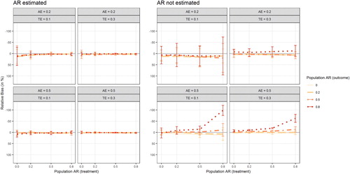
Figure 6 depicts the relative bias in the TE (computed as the difference between estimated TE and population TE, relative to the population TE and multiplied by 100) for the simulated conditions. Note that when the AR(1) population parameters are explicitly estimated (left panel), there seems to be no discernible bias in the estimation of the TE. When the AR(1) parameters are fixed to zero, a substantial downward bias in the TE was observed when both true autoregressive parameters were large (0.8) and the AE was large (0.5), too. That is, when the encouragement has a strong effect on treatment behavior, but the respective treatment behavior and outcome are highly inert, the TE is substantially downward biased.

Figure 6. Figure displays the relative bias in the estimation of the treatment effect as a function of the population AR(1) effect in treatment behavior (x-axis), the population AR(1) effect in the outcome (separate lines), the population adherence effect (AE; separate rows), and the population treatment effect (TE; separate columns) Results are plotted separately for models in which the AR(1) effects were explicitly estimated (left panel) or fixed to zero (right panel). Error bars indicate 95% confidence intervals. Note that the y-axis has been reverted.

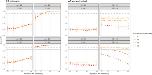
Figure 7 shows power estimates of detecting a significant TE (please note that “significant” in this model using a Bayesian estimator means that the 95% credible interval does not include zero). When the AR(1) effects are estimated, power increases with increasing population AR(1) in the behavior, but is unaffected by population AR(1) in the outcome. When the autoregressive parameters are fixed to zero (right panel) power is primarily affected by the false fixations of the AR(1) effect of the outcome: power is markedly lower in conditions with falsely fixated large AR(1) effects of the outcome. Neglected AR(1) effects in the treatment behavior affected power to a lesser extent, except in the condition with high AE and high TE.

Figure 7. Figure depicts power of the treatment effect as a function of the population AR(1) effect in treatment behavior (x-axis), the population AR(1) effect in the outcome (separate lines), the population adherence effect (AE; separate rows), and the population treatment effect (TE; separate columns) Results are plotted separately for models in which the AR(1) effects were explicitly estimated (left panel) or fixed to zero (right panel). Error bars indicate 95% confidence intervals. Gray horizontal lines mark 80% power (solid line) and 90% power (dashed line).

Discussion

With the present work, we show how an experimental approach can be used to investigate the causal relations that potentially underlie the coupling of variables at the within-person level, and how the implementation as an encouragement design can make such an approach applicable in a broad range of realistic scenarios. The results of the simulation studies show that IVE of the causal effects in such encouragement design studies is possible under feasible (regarding design dimensions) and realistic (regarding adherence to encouragements) conditions. This renders the proposed design potentially applicable to a wide array of research topics. In the following, we will summarize and discuss results of the simulations, and suggest possible extensions, as well as address potential complications and limitations of the approach.

Results of simulation studies

Results of our simulations studies suggest that if the true population model is fitted to the data (i.e., non-zero random variances are estimated, non-zero autoregressive effects are estimated), good statistical power and negligible bias in parameter estimates can be achieved with design dimensions that seem realistic for studies in psychological research. Effectively, it was the overall sample size (i.e., the product of the number of participants and the number of occasions) that mattered in terms of power. That is, having 100 observations from 20 participants works similarly well as having 20 observations from 100 participants. In prior simulation work, increasing the number of Level 2 units has been reported to have a stronger effect on power than increasing the number of Level 1 units (Bolger & Laurenceau, 2013). Potentially, our study yielded equal effects of both sample sizes because in our simulations, within-person variance was approximately equal to (or slightly larger than) between-person variance. If one of these sources of variance dominates the other, statistical power might depend relatively more on the sample size at the corresponding level. As a general conclusion, it seems that being able to get total numbers of observations (persons x occasions) in the order of thousands using intensive longitudinal designs, therefore puts the within-person encouragement design in the ballpark of sample sizes used in between-person studies in that IVE has already been successfully used to analyze the effects of treatments implemented via encouragements.

Besides the obvious influence of the size of the true treatment effect and the overall sample size on statistical power, the rate of adherence to the encouragements clearly was a strong influential factor. It should be noted that in conditions where the total number of observations (i.e., N × T) was 2000 or larger, adherence effects of d = 0.50 consistently resulted in good power to detect treatment effects of at least 0.30. To illustrate the size of an adherence effect of 0.50, we transformed this metric into the common language effect size indicator (McGraw & Wong, 1992). Note that treatment behavior was operationalized as continuous (normally distributed) variable in the simulations studies (i.e., as a proclivity to show a certain behavior). An effect size of d = 0.50 in this case means that the proclivity to show the treatment behavior is higher when encouraged, in comparison to not being encouraged, in about 64% of the observations (Grissom, 1994). Note that if encouragements had no effect (d = 0), this number would be 50%. This emphasizes that the adherence rates necessary to make our approach work in realistic conditions (e.g., N = 50, T = 50) are far from close-to-perfect adherence, and therefore likely to be achievable in real-life situations. Furthermore, we also found that larger random variance in the adherence effect was associated with higher power for the treatment effect. A large random variance in the adherence effect indicates that individuals differ in the extent to which they comply with the encouragement. All other things being equal, this leads to more variance in the treatment that is caused by the encouragement. That is, a random effect in the adherence effect increases the variance of the predictor “treatment” (the part in treatment that is caused by the encouragement), which should be associated with larger power to detect the (average) effect of (experimentally induced) treatment on the outcome – the pattern observed in our simulation studies.

Our results further showed that correct specification of the model on both Level 2 and Level 1 is key to obtaining unbiased parameter estimates of the TE. Regarding the former, under false model specification (i.e., random effect variances were not estimated), the TE was substantially biased downward if both, the adherence was low (less than 0.5) and sample size was small. However, with total sample size of 2000 or higher, and adherence effect of 0.30 or higher, the amount of bias was only small (<4%) and probably unproblematic from a pragmatic applied perspective (e.g., an estimated treatment effect of 0.31 vs. a true treatment effect of 0.30).

Another aspect that can further complicate parameter estimation, while at the same time also may be of considerable substantive interest, is the possibility of sequential dependencies (i.e., autoregressive effects) in the variables of the model at Level 1. While the encouragements are free of sequential dependencies because of their randomized nature, the treatment and outcome variable might exhibit autoregressive dynamics. If having overcome the reluctance to exercise on one day increases the likelihood of exercising also on the next day, for example, this would imply a positive lag-1 autoregressive effect of the treatment. Regarding mood as a potential outcome variable, “emotional inertia” (Kuppens, Allen, & Sheeber, 2010) might make the effects of the treatment on affect, or of other factors that produce variation in affect, carry over to the next day. Results from Simulation Study 2 showed that if these autoregressive effects are falsely constrained to zero, the estimation of the TE can be affected by substantial bias, but only if both autoregressive effects are strong (0.80) and the adherence effect is of medium size (0.50). Under less strong autoregressive effects (0.50 or lower), there was no noticeable bias of the TE even if this autoregressive effect was erroneously neglected.

There were, however, noticeable decrements in statistical power associated with the TE when model misspecifications occurred. Power was in most conditions higher when (true non-zero) random variances were estimated compared to when they were erroneously fixed to zero (Simulation 1). Similarly, power was higher when (true non-zero) auto-regressive effects were estimated compared to when they were erroneously fixed to zero (Simulation 2).

In summary, under realistic conditions (medium sized adherence to the encouragement; total number of observations exceeding 2000), largely unbiased estimates of the treatment effect can be obtained, and the models are adequately powered to detect at least medium sized treatment effects. In case of model misspecifications on Level 1 (not estimating true non-zero autoregressive effects) or Level 2 (not estimating true non-zero random variances), parameter estimates may be biased in some conditions, but this bias is primarily obtained in already unfavorable conditions (small sample sizes, low adherence to the encouragement) or in conditions of extreme misspecifications (very large autoregressive effects). Nevertheless, power is attenuated if the model is mis-specified; therefore, attempts need to be made to correctly specify the model. Falsely fixating true non-zero random variances to zero has been shown to be associated with worse performance in the estimation of fixed effects compared to attempting to estimate truly zero random variances in a simulation study by Baird and Maxwell (2016). Extending these findings to the scenario investigated here leads to the advice that researchers utilizing our proposed approach should start by fitting a model with random variances and autoregressive effects if feasible.

An aspect that might play an important role, both in terms of substantive interest and of its effect on the feasibility and quality of parameter estimation, is that random effects may also be correlated. From substantive perspectives, it may, for example, be of interest whether individual differences in adherence are associated with individual differences in the strength of the TE. From the perspective of parameter estimation, it is to be expected that the inclusion of covariance parameters increases the number of convergence problems and improper solutions. For lower level mediation models, the covariance between the random effect of a predictor on a mediator and the random effect of the mediator on the outcome has been shown to play a pivotal role for the estimation of the total effect and the amount of mediation (Kenny, Korchmaros, & Bolger, 2003). The model proposed in the present work is conceptually similar to a lower level mediation model (with the behavior as the assumed mediator of the effect of the encouragement on the outcome), but it is different with regard to at least two aspects: First, our model acknowledges the possibility of shared endogenous influence on the behavior/mediator and the outcome by modeling these influences as a covariance of the respective residual terms. Second, the central effect in our model is the TE (the effect of behavior on outcome), whereas it is the indirect effect in a (lower level) mediation model. Hence, the role of covariance between random effects of AE and TE for the estimation the TE needs to be explored in future research.

Potential problems

Potential problems of the proposed approach result from violations of general assumptions involved in IVE, violations of additional assumptions associated with the time-sequential nature of the data, and further statistical and practical issues. A first general problem associated with IVE is the potential weakness of the instrumental variable. As shown in our simulations, very small AEs indeed can lead to estimation problems and unsatisfactory statistical properties. As these problems can be compensated for by large enough numbers of participants and/or occasions, the general conclusion regarding the “weak instrument” issue is that design dimensions need to match the expected adherence rates.

While this first general assumption of IVE can be empirically tested, the second assumption of the so-called “exclusion restriction” cannot be verified empirically, but only be argued for theoretically. For this assumption to be met, it is necessary that any relation of the instrument to the outcome is solely mediated through the treatment. It would be violated, for example, if encouragements to exercise (e.g., go for a run) lead to alternative health behavior (e.g., taking a relaxing break) on days when the encouraged behavior cannot be shown. If the alternative behavior has an effect on the outcome, the resulting alternative path from the encouragement to the outcome will bias the estimate of the treatment effect in a model which does not account for this alternative path. There are two general possibilities of dealing with such alternative paths, if they cannot be ruled out based on theoretical considerations. The first one is based on trying to measure the relevant variables and include the missing paths into the model. If this is not possible, the second possibility is to run sensitivity analyses that evaluate how strong (the sum of) such alternative paths would need to be to reduce the resulting estimate of the TE to a value that would not be of practical relevance any more.

When using the IVE approach at the within-person level, the constrained interpretation of the LATE (of only pertaining to the hypothetical subpopulation of participants whose treatment behavior is determined by the instrumental variable) relates to the population of occasions. Here, the LATE provides an estimate of the causal effect of the treatment only for the subset of occasions on which participants would adhere to either of the two possible conditions (i.e., to show, or not to show, the treatment behavior). For occasions on which participants would show (or not show) the treatment behavior irrespective of the provided encouragement condition, the hypothetical treatment effect remains unknown. This is a restriction that needs to be considered in the interpretation of results from an IVE analysis of studies with an encouragement design. We do not consider this restriction to be a major drawback, however, as in many applications, being able to generalize results to situations in which behavior can be (experimentally) controlled will ensure sufficient practical relevance.

Additional problems associated with the time-structure of the data in a within-person study stem from the stationarity assumptions that are required in the analysis of time series data. Over the course of an encouragement study, adherences rates may drop due to losses of motivation and the strength of the TE might increase due to increasing practice with implementing the treatment, to name just two examples. How well parameter estimates from models with implied stationarity assumptions recover the true average values of time-varying parameters therefore is another question for future simulation work. Similarly, matters could be more complicated by autoregressive effects of higher order and by cross-regressive effects, for example, if encouragement on day t has a delayed effect on treatment behavior at day t + 1.

A practical problem that directly affects the statistical properties of the parameter estimation is that it may not be possible to set the probability of providing encouragements to 0.50. It can be expected that deviations from this optimal rate (which we used throughout our simulations) will lead to loss of power – while generally being a possible option. For example, it seems reasonable to assume that working with a base rate of encouragements smaller than 0.50 is preferable to constraining the sample of occasions a-priori to one that has fewer occasions, but allows for a .50 base rate. The effects of working with different base rates of encouragement also require additional simulation work, however.

Regarding the practical implementation of an encouragement design, as well as the estimation and interpretation of effects, it is optimal if the effect of the treatment behavior arises pretty quickly, but dissipates until the next occasion where an encouragement can be provided. This may be realistic, for example, for the effects of certain sleep behaviors, which may have effects that can be measured throughout the subsequent day, but not beyond the subsequent night, in which the treatment behavior then again can be shown. If the time course of rise and decay of an effect is faster, the measurement of the outcome simply needs to be close enough in time to capture the effect. If the time course is slower, however, the spacing of occasions where encouragements can occur either needs to be wide enough for TEs to vanish, or a modeling approach that takes this time course of effects into account needs to be chosen. Also, if there is accumulation of (side) effects over time, or complex interactions for certain patterns of treatment behavior (e.g., knee problems that only occur if somebody goes for a run on at least three consecutive days), this needs to be taken care of either in the design (e.g., by constraining the random sequences of encouragements) or in the analytical model.

In general, examples of treatments that have relatively immediate but transient effects, and thereby qualify for being evaluated using within-person encouragement designs, may be found in several fields of behavioral science. In health psychology, everyday behaviors in the areas of, for example, nutrition, sleep hygiene, and physical exercise render themselves highly suited. In sports medicine, the effects of warming up, stretching, and other pre- or post-exercise activities seem to be appropriate candidates. In clinical psychology, the effectiveness of relaxation or mindfulness exercises could be investigated in the everyday contexts that these exercises are targeting. In educational science, behaviors that can support learning, like planning or self-instruction, could also be in the focus of within-person interventions using encouragements. Even in cases where the treatment behavior is meant to be learned and automatized over time and practice, like implementation intentions or self-regulation strategies, the effectiveness of the behavior may be studied using encouragements during an initial phase in which it is not yet overlearned.

Possible extensions of the model

The basic model that we used in our simulations can be extended in a number of ways. Being implemented in a SEM framework, it is possible, for example, to include latent variables based on measurement models. This may be of particular interest for the outcome constructs, which could be operationalized with several indicator variables and thereby allowing for an estimation of TEs that are not attenuated by unreliability of the outcome measure. Also, the SEM framework allows for the inclusion of further variables at Level 1. As discussed above, this could be used to control for alternative paths mediating effects from encouragement to outcome. It could also be used to control for irrelevant variance in the outcome variable, or to account for time-related trends in the data.

Similarly, covariates at Level 2 could be included. This could be done, for example, in attempts to explain individual differences in the adherence to encouragements, or the effectiveness of the treatment, with person-level variables like personality traits or demographic variables. Such individual differences also could be the target of latent class analyses with the aim to identify groups of participants that differ in their patterns of within-person associations (cf. Neubauer, Dirk, & Schmiedek, 2019). The possibility to identify and further explore individual differences in TEs, generally has to be seen as a great advantage of our proposed approach. We note, however, that targeting these Level 2 research questions might require larger sample sizes, in particular larger sizes on Level 2. Schultzberg and Muthén (2018) tested several dynamic SEMs in a simulation study and examined the effects of Level 1 and Level 2 sample size on estimation quality. Whereas in models primarily targeting Level 1 associations, smaller sample sizes (e.g., N = 50 − 100) lead to adequate results, larger Level 2 sample sizes were required for models that targeted associations on Level 2.

A further option that we have not addressed here in detail is that, in principle, the within-person encouragement approach could also be used in single-case studies. The DSEM framework allows for the estimation of time series from single participants, so that model estimation could be done in the same framework as we used here. Note, however, that this likely will require very large numbers of occasions from the single participant. While such “extensive intensive” longitudinal designs might be beyond the possibilities of many research applications, the increased availability and use of smartphone apps to monitor and optimize one’s behavior continuously over a very long time renders such options not totally unrealistic.

Conclusions

There are numerous behaviors that people can repeatedly choose to show (or not to show) in their everyday lives and that are thought to be beneficial, for example, for cognitive performance, mood, or other aspects of psychological or physiological well-being. Prime examples are the kinds of behaviors health psychologist aim to promote. Probing such potential effects by showing the behavior on selected occasions likely is a common way that even laypersons use when they have the goal to evaluate whether the behavior really holds up to promise for themselves. The effects observed in such quasi-experimentation on the within-person level, however, can easily be confounded with third variables (e.g., having slept well leading to an increased likelihood of exercising and also to better cognitive performance, spuriously increasing the observed relation of exercise and cognition), so that observational data on within-person couplings of treatment and outcome variables do not necessarily provide valid information on causal effects. Strict random manipulation, however, will often be difficult or even impossible to implement in daily life. Our proposed within-person encouragement approach opens a practical compromise by taking advantage of the fact that the experimental introduction of at least some amount of variation in behavior – via randomly timed encouragements – can be used to estimate causal effects, and individual variation therein, in everyday contexts. Together with technical advancements in monitoring and prompting behavior, as well as ambulatory assessment of outcome variables, this approach promises to open up a whole new area of behavioral research on causal effects in everyday life.

Article information

Disclosure statement: Each author signed a form for disclosure of potential conflicts of interest. No authors reported any financial or other conflicts of interest in relation to the work described.

Ethical Principles: The authors affirm having followed professional ethical guidelines in preparing this work. These guidelines include obtaining informed consent from human participants, maintaining ethical treatment and respect for the rights of human or animal participants, and ensuring the privacy of participants and their data, such as ensuring that individual participants cannot be identified in reported results or from publicly available original or archival data.

Funding: This work was supported by Grant 2016-1245-00 from the Jacobs Foundation.

Role of the Funders/Sponsors: None of the funders or sponsors of this research had any role in the design and conduct of the study; collection, management, analysis, and interpretation of data; preparation, review, or approval of the manuscript; or decision to submit the manuscript for publication.

Acknowledgments: The ideas and opinions expressed herein are those of the authors alone, and endorsement by the authors’ institutions or the Jacobs Foundation is not intended and should not be inferred. This research was supported by funding from the Jacobs Foundation as part of the project UPWIND (Understanding and Improving Within-Child Dynamics in the School Context). Central ideas included in the present work were presented at the 58th Conference of Experimental Psychologists (TeaP) in Heidelberg (2016) and in a seminar of the Network for Intrapersonal Research on Education (NIRE), University of Oxford (2016).