Methods for Constructing Normalised Reference Scores: An Application for Assessing Child Development at 24 Months of Age

Abstract

The use of the lambda-mu-sigma (LMS) method for estimating centiles and producing reference ranges has received much interest in clinical practice, especially for assessing growth in childhood. However, this method may not be directly applicable where measures are based on a score calculated from question response categories that is bounded within finite intervals, for example, in psychometrics. In such cases, the main assumption of normality of the conditional distribution of the transformed response measurement is violated due to the presence of ceiling (and floor) effects, leading to biased fitted centiles when derived using the common LMS method. This paper describes the methodology for constructing reference intervals when the response variable is bounded and explores different distribution families for the centile estimation, using a score derived from a parent-completed assessment of cognitive and language development in 24 month-old children. Results indicated that the z-scores, and thus the extracted centiles, improved when kurtosis was also modeled and that the ceiling effect was addressed with the use of the inflated binomial distribution. Therefore, the selection of the appropriate distribution when constructing centile curves is crucial.

Keywords:

• Reference equations
• LMS method
• centiles
• norms tables
• child development

Introduction

Maximizing child development is a public health priority as early life events can have long-term consequences for individuals and populations. Although cognitive and language development continue throughout childhood and adolescence, delayed development in early childhood, in the first three years of life, is a risk factor for a range of developmental problems and disorders that can have an adverse impact on a child’s lifelong health and wellbeing (Black et al., 2017). Monitoring early development is therefore essential for identifying children with delay in order to ensure that they receive timely intervention to minimize the impact of impairments and improve life chances (Engle et al., 2011). This requires the use of valid and reliable assessments that yield norm-referenced age-standardized scores for quantifying development and classifying delay relative to children in the general population (American Academy of Pediatrics. Committee on Children With Disabilities. Developmental Surveillance and Screening of Infants and Young Children, 2001).

Routine developmental assessment at two years of age, in particular at 24 months of age, is recommended for clinical populations of children at high risk of developmental disorders, such as children born very preterm (i.e. before 30 weeks of gestation) (NICE Guideline: Developmental follow-up of children and young people born preterm, 2017; Report of a BAPM/RCPCH Working Group: Classification of health status at 2 years as a perinatal outcome, 2008), infants with congenital heart disease (Marino et al., 2012) and other hospitalized newborns (International Consortium for Health Outcomes Measurement (ICHOM), Preterm and Hospitalized Newborn Health Group, NEO Standard Set, 2020; European Foundation for the Care of Newborn Infants (EFCNI), European Standards of Care for Newborn Health, 2018).

The Parent Report of Children’s Abilities-Revised (PARCA-R) provides one such measure for assessing children’s cognitive and language development that has been recommended for use in routine neurodevelopmental follow-up, to assess development at 24 months of age. This brief parent-completed questionnaire (Johnson et al., 2004; Saudino et al., 1998) has been used extensively for clinical and research purposes (Beardmore-Gray et al., 2022; Dorling et al., 2019; Draper et al., 2020; Gupta et al., 2021; Johnson et al., 2015). Although assessments are targeted to occur specifically at 24 months of age, obtaining timely follow-up data is challenging (e.g. due to delays in parents completing or returning the questionnaire, or difficulties scheduling face to face assessments on time), therefore it is quite common for such assessments to occur when children are aged around 24 to 27 months. The PARCA-R has previously been shown to have good reliability and validity and, using empirically derived cutoff scores, good diagnostic utility for identifying preterm-born children with moderate to severe delay on an examiner-administered test (Blaggan et al., 2014; Cuttini et al., 2012; Johnson et al., 2004; Johnson et al., 2008; Martin et al., 2012; Martin et al., 2013; Picotti et al., 2020). The PARCA-R consists of three sub-scales: (i) non-verbal cognition (range 0–34), (ii) vocabulary (range 0–100) and (iii) sentence complexity (range 0–24). The two latter scales are combined to produce a “language development” score (range 0–124), which is then summed with the “non-verbal cognitive score” to produce an overall “parent report composite” (PRC) score (range 0–158). The PARCA-R has been translated and validated in other European languages (Cuttini et al., 2012; Picotti et al., 2020; Vanhaesebrouck et al., 2014) and is widely used as a developmental assessment in clinical services and as an outcome measure in clinical trials (Abbott et al., 2017; Brocklehurst et al., 2011; Dorling et al., 2019; “Infant Collaborative Group. Computerized interpretation of fetal heart rate during labor (INFANT): a randomized controlled trial,” 2017; Marlow et al., 2006) and observational studies (Draper et al., 2020; Field et al., 2016; Martin et al., 2012). However, the lack of standardized scores for comparing a child’s developmental level with that of the norm limited its ability to identify children with subtle delays and to quantify progress across the full spectrum of development. Moreover, since development may increase even daily over this narrow age range, the use of the same reference scores to make individual decisions may lead to the misclassification of a part of the sample. Therefore, in 2019, we undertook a standardization study (Johnson et al., 2019) to produce reference scores in children from four different age groups (i.e. 24, 25, 26 and 27 months of age) for the PARCA-R to facilitate its use as a continuous outcome measure and as a universal developmental assessment. Within this scope we aimed in this paper to present the methodology to follow when constructing standardized scores and highlight issues that could be vital if ignored when identifying a population in need of intervention.

Age-related normalized reference ranges are commonly calculated using the normal distribution, as opposed to rank-order distributions, that allow for the generalization of the results through the calculation of the normalized percentile curves. Within psychometrics the percentiles, that are equivalent to z-scores, can subsequently translated to standard scores allowing the comparison with other standardized tests. The lambda(λ)-mu(μ)-sigma(σ) (LMS) method (Cole & Green, 1992; Cole et al., 2009) has been extensively used in different clinical settings (Kobayashi et al., 2016; Norris et al., 2018; Quanjer et al., 2012) for that purpose. It was developed as an extension of the standard linear regression model to allow greater flexibility when the modeling assumptions are not satisfied (Cole & Green, 1992). The basis of this method is that the main assumptions for normality and homoscedasticity of a linear model will be satisfied when a suitable transformation has been applied to the response variable (Box & Cox, 1964). The latter can be achieved by modeling the skewness (λ), the mean (μ) and the standard variation (σ) and using their estimated values. This allows the modeling of nonsymmetrical distributions, which are common in age-related scales such as those measuring cognitive development (Gluhm et al., 2013; Hayat et al., 2014). Further advances in the use of the LMS method (Rigby & Stasinopoulos, 2004) also allow for modeling the fourth moment (i.e. kurtosis, τ) of the distribution of the response variable.

However, the main modeling assumption of conditional normality of the errors should be satisfied in the LMS method, which is not often the case in age-bound scales that are discrete and that often show strong ceiling and, in some cases, floor effects (Uttl, 2005). These elements can violate the main modeling assumption and lead to distorted fitted parameters and biased fitted centiles. A potential solution to these problems is the generalized additive model for location, scale and shape (GAMLSS), which has been developed to allow even greater flexibility by the specification of an appropriate probability distribution relevant to the response variable (Rigby & Stasinopoulos, 2005). In addition, it has been suggested that probability distributions other than the Normal distribution might be more suitable to address these limitations (Hossain et al., 2016; Muniz-Terrera et al., 2016).

Although the GAMLSS has been implemented by the World Health Organization to produce growth charts for children (WHO Multicentre Growth Reference Study Group. WHO Child Growth Standards: Growth velocity based on weight, length and head circumference: Methods and development, 2009), it is unclear whether these advances have been applied in different settings and, in particular, in psychometrics where the construction of norms tables and age standardized scores is common (Bayley, 2006; Brooks et al., 2009). The PARCA-R parent report composite (PRC) score is such a discrete scale, bounded within a certain range (0–158). As such, an exploration of the appropriate method for producing reference scores is needed. In this paper, we investigate different distribution families when modeling the association between the PRC scores and age whilst producing standardized scores for assessing cognitive and language development using the PARCA-R.

Methods

In our analyses, three distribution families were considered to model the PRC score as a function of age and produce reference scores: a) the Box-Cox-Cole-Green (BCCG) distribution, which is the common LMS method; b) the Box-Cox power exponential (BCPE) distribution, which is an extension to the LMS method and allows to model kurtosis; and c) the beta inflated distribution bounded at [0, 1] (i.e. inclusive of both 0 and 1, BEINF01). Analyses were performed in R version 3.4.3 (“R Core Team. R: A language and environment for statistical computing,” 2017) using the package “GAMLSS” (Rigby & Stasinopoulos, 2005) and plots were produced using the package “ggplot2” (Wickham, 2009).

General model for centile estimation

The implementation of the GAMLSS framework (Rigby & Stasinopoulos, 2005) offers the ability to fit different probability distributions to the response variable, so that an appropriate distribution can be chosen from different alternatives. Let us assume that Y is the response variable, X is the explanatory variable and $\theta =({\theta }_1,\mathrm{ }{\theta }_2,\mathrm{ }\dots ,\mathrm{ }{\theta }_k)$ is the vector of K distribution parameters. A general model for creating the centiles for Y conditional on the value x of X will be: $$Y\sim D\left(\theta \right)$$ (1) $$g_k\left({\theta }_k\right)={\eta }_k={{\rm X}}^{\prime }{\beta }_k+\sum _{j=1}^{J_k}{h}_{jk}\left(x_{jk}\right),\mathrm{ }k=1,\mathrm{ }2,\mathrm{ }\dots ,\mathrm{ }K,\mathrm{ }$$(1) where D is the assumed distribution, $k$ is the total number of distribution parameters, with the first four representing $mu\mathrm{ }\left(\mu \right),\mathrm{ }\mathit{sigma}\mathrm{ }\left(\sigma \right),\mathrm{ }\mathit{lambda}\mathrm{ }\left(\lambda \right)\mathrm{ }\mathit{and}\mathrm{ }\mathit{tau}\mathrm{ }\left(\tau \right),$ $g_k$ is the link function, ${\eta }_k$ is the linear predictor, $X^{\prime }{\beta }_k$ is the vector of linear terms of length $J_k$ and ${\sum }_{j=1}^{J_k}{h}_{jk}(x_{jk})$ is a smooth non-parametric function, denoted by $h_{jk}$ (e.g. p-splines, cubic splines, fractional polynomials) of the explanatory variable $X_{jk}$ evaluated at $x_{jk}$ in the regression model. Using the GAMLSS, up to four parameters of the response variable distribution, which are usually characterized as location (denoted by μ, the approximate mean), scale (denoted by σ, the approximate standard deviation) and shape (skewness denoted by λ and kurtosis by τ) parameters, can be modeled with four corresponding equations equivalent to equation (1) above, defining the distribution parameters.

According to the nature of the response variable, there are three distinct types of distribution families: continuous, discrete and mixed distributions. Continuous distributions are usually defined on the (-$\mathrm{\infty },\mathrm{ }+\mathrm{\infty }),$ (0, $+\mathrm{\infty }),$ or (0, 1) range and are linked to each other through the log or logit transformation or their inverse. Discrete distributions refer to count values and are usually defined on the (0, 1, 2,…, i) range where i can be a known finite value or infinite. Mixed distributions are continuous distributions where the range of the response variable has been extended to include some discrete values with non-zero probabilities. In this paper, we focus on the continuous and mixed distributions, describing three approaches to specify the model and exploring their use for centile estimation where the outcome is bounded.

Centile estimation for continuous distributions

Continuous distributions can be symmetric, negatively or positively skewed. The LMS method (Cole & Green, 1992), implemented through the Box-Cox-Cole-Green (BCCG) distribution in GAMLSS (Rigby et al. 2020) has been widely used to produce centile references by modeling mu $(\mu ),$ sigma $(\sigma )$ and lambda $(\lambda ).$ According to its principles, the distribution of a positive (Y > 0) response variable is defined through the transformed random variable Z given by: (2) $$z=\{\begin{array}{c}\frac{1}{\sigma \times \lambda }\left[{\left(\frac{Y}{\mu }\right)}^{\lambda }-1\right],\mathit{\text{ if λ}}\ne 0\\ \frac{1}{\sigma }\log \hspace{0.17em}\left(\frac{Y}{\mu }\right),\mathit{\text{ if λ}}=0\end{array},\mathrm{ }$$(2) where the transformed variable Z is a z-score that follows a truncated standard normal distribution (i.e. Z ∼ N(0, 1)). In this case, the probability density function denoted by $\mathit{BCCG}(\mu ,\mathrm{ }\sigma ,\mathrm{ }\lambda )$ is defined by: (3) $$f_Y\left(y\mathrm{|\mu },\mathrm{ }\sigma ,\mathrm{ }\lambda \right)=\frac{y^{\lambda -1}\mathrm{e}\mathrm{xp}(-\frac{1}{2}{z}^2)}{{\mu }^{\lambda }\sigma \sqrt{2\pi }\Phi \left(\frac{1}{\sigma \left|\lambda \right|}\right)},\mathrm{ }$$(3) where z is given from equation (2) above, and Φ() is the cumulative distribution function of the standard normal distribution.

However, the distribution of the outcome may also be leptokurtic (thicker/heavier tails than the normal distribution) or platykurtic (thinner/lighter tails than the normal distribution) and this shape is not captured with the BCCG distribution which is suitable for a mesokurtic (i.e. normal) distribution. To account for the shape of the distribution another family has been introduced as an extension to the LMS method. This extended distribution that also models kurtosis (tau, τ) is called the Box-Cox power exponential distribution (Rigby et al., 2020), denoted as $\mathit{BCPE}\left(\mu ,\mathrm{ }\sigma ,\mathrm{ }\lambda ,\mathrm{ }\tau \right)$ and its probability density function is defined by: (4) $$f_Y\left(y\mathrm{|\mu },\mathrm{ }\sigma ,\mathrm{ }\lambda ,\mathrm{ }\tau \right)=\frac{y^{\lambda -1}{f}_Z\left(z\right)}{{\mu }^{\lambda }\sigma F_Z\left(\frac{1}{\sigma \left|\lambda \right|}\right)},\mathrm{ }$$(4) where $f_Z\left(z\right)$ and $F_Z(z)$ are the probability and cumulative distribution functions of a random variable Z having a standard power exponential distribution, such as Z ∼ PE(0, 1, tau) with power parameter tau > 0.

Centile estimation for mixed distributions

Whilst the distributions outlined above are likely to be appropriate for scores that do not exhibit ceiling and floor effects, for example the Mild Cognitive Impairment Questionnaire (Dean et al., 2018), they cannot adequately allow for such effects where do they exist, for example the Mini Mental State Examination (Muniz-Terrera et al., 2016) or the PARCA-R (Johnson et al., 2004; Saudino et al., 1998). Mixed distributions are mixtures of continuous and discrete distributions and they include the zero adjusted distributions defined on the [0; $\mathrm{\infty }$) interval and the specific case of inflated distributions defined on the [0; 1] interval. Beta inflated distributions (Rigby et al., 2020) fall in the latter category, in which the values of the response variable lie within 0 ≤ y ≤ 1 and they are a mixture of three components: a discrete value 0 with probability $\mathrm{ }{p}_0,$ a discrete value 1 with probability $\mathrm{ }{p}_1,$ and a continuous beta distribution $BE\left(\mu ,\mathrm{ }\sigma \right)\mathrm{ }$ on the unit interval (0; 1) with probability $\mathrm{ }\left(1-p_0-p_1\right).\mathrm{ }$ The probability function of the inflated beta distribution at 0 and 1, denoted by $\mathit{BEINF}01\left(\mu ,\mathrm{ }\sigma ,\mathrm{ }\lambda ,\mathrm{ }\tau \right)\mathrm{ }$ is defined by: (5) $$f_Y\left(y\mathrm{|\mu },\mathrm{ }\sigma ,\mathrm{ }\lambda ,\mathrm{ }\tau \right)=\{\begin{array}{c}{p}_0,\mathit{\text{ if y}}=0\\ \left(1-p_0-p_1\right)\frac{1}{B\left(\alpha ,\mathrm{ }\beta \right)}{y}^{\left(\alpha -1\right)}{\left(1-y\right)}^{\left(\beta -1\right)},\mathit{\text{ if }}0<y<1 \\ p_1,\mathit{\text{ if y}}=1\end{array}$$(5) , where $$\alpha =\frac{\mu \left(1-{\sigma }^2\right)}{{\sigma }^2},\mathrm{ }\beta =\frac{\left(1-\mu \right)(1-{\sigma }^2)}{{\sigma }^2},\mathrm{ }$$ $$p_0=\frac{\lambda }{(1+\lambda +\tau )},\mathrm{ }{\mathit{and}\mathrm{ }p}_1=\frac{\tau }{(1+\lambda +\tau )},\mathrm{ }\mathit{for}\mathrm{ }0\le y\le 1$$

It becomes apparent that the $\mathit{BEINF}01\left(\mu ,\mathrm{ }\sigma ,\mathrm{ }\lambda ,\mathrm{ }\tau \right)$ has parameters:

$\mu =\frac{\alpha }{(\alpha +\beta )}$ and $\sigma =\frac{1}{\sqrt{(\alpha +\beta +1)}},$ with $E\left(y\right)=\frac{\tau +\mu }{(1+\lambda +\mu )}$.

Any response variable bounded with both a lower and upper limit can be transformed so that the transformed values ( $y_T$) lie within 0 ≤ y ≤ 1. Therefore, in this analysis, the PRC score was transformed to the [0, 1] range by dividing each score with the total number of questions, and hence produce the proportion of answers for which a child received a score of 1 For example, a raw score of 1 out of the 158 in the scale is equivalent to 0.0063 in the transformed 0 to 1 scale and corresponds to 0.63% of the total raw score.

Model selection

As our aim was to produce age-specific standardized scores for PRC, separately in boys and girls, we included age (in days) as the only explanatory variable of the four parameters defining the location, scale and shape of the distribution (i.e. $\mu ,\mathrm{ }\sigma ,\mathrm{ }\lambda ,\mathrm{ }\tau$). Then a series of models were tested within each distribution family examining whether age contributed significantly in predicting all the parameters of each model. To derive the standardized scores, we adopted the following strategy considering:

1. the distribution of the response variable, that is the BCCG, the BCPE and the BEINF01 alongside the relevant link function,

2. whether age is a significant predictor for each parameter (i.e. $\mu ,\mathrm{ }\sigma ,\mathrm{ }\lambda$ and $\tau$) or the parameter is constant across the data, and

3. whether a smoothing function for age should be included.

The link function allows, if necessary, for an appropriate transformation of the response variable to model its linear association with the linear predictors in the model. Before selecting the link function, one should examine whether the main assumptions of normality and linearity are satisfied with the identity link function. If the assumptions are not met, alternative link functions can be tried for each parameter ( $\mu ,\mathrm{ }\sigma ,\mathrm{ }\lambda$ and $\tau$) and the preferred link function should be the one which gives the smallest value of the information criteria used for model selection. With respect to the set of link functions, we used the default link functions as described by Rigby and colleagues (Rigby et al., 2020), shown in Table S2 (OLS) as it was found to produce the smallest value of the generalized Akaike information criterion.

Table 2. Distribution of z-scores derived from the best selected models from each distribution family, in boys (n = 3,321) and girls (n = 3,081).

	Boys			Girls
	BCCG	BCPE	BEINF01	BCCG	BCPE	BEINF01
	M1.3	M2.6	M3.3	M1.3	M2.8	M3.1
Min.	−3.11	−4.23	−3.89	−4.17	−4.35	−4.21
P50 (P25; P75)	−0.02 (−0.75; 0.77)	−0.07 (−0.68; 0.59)	−0.11 (−0.72; 0.63)	−0.08 (−0.77; 0.77)	−0.08 (−0.65; 0.60)	−0.09 (−0.71; 0.67)
Mean (SD)	0.004 (0.99)	−0.03 (0.99)	−0.008 (1.00)	−0.02 (1.01)	−0.02 (0.99)	−0.004 (1.00)
Max.	2.08	2.57	3.41	2.09	2.91	4.02

To model age-related trends in development, smoothing functions were applied to remove the effects of sampling and measurement variation across the age range. The use of splines allow for a smoothed representation of the non-linear effect (if present) of age on the response variable. Although there are different ways to incorporate a smoothing function (e.g. cubic splines, kernel estimation, locally weighted regression) we opted to use the penalized beta (PB) splines that allow the predictive line to follow the data, ensuring that knots are well spread across the data, but incorporating a penalty for doing so and also are unconstrained at the boundary knots. Then the appropriate smoothing function and the optimum degrees of freedom for all the parameters of the model was selected on the basis that minimized the value of the information criteria used for model selection (Eilers & Marx, 1996).

Significance level and information criteria

First, the models were selected by taking into account the significant contribution of age in each of the parameters modeled. Then, for models in which age contributed significantly in each of the modeled parameters, a balance between the reduction of global deviance (D) and the generalized Akaike information criterion (GAIC; Akaike, 1983), was considered for final model selection. Global deviance is used to compare nested models and is defined as D= -2 × logLikelihood. The closer the deviance is to zero the better the model’s fit. The GAIC was additionally considered to examine the parsimony of the model and to avoid under- or over-fitting. It is defined as GAIC = deviance + df × k, where df are the total model degrees of freedom and k is a penalty for each effective degree of freedom that is used in a model. Thus GAIC penalizes models with more parameters and a model with the smallest GAIC value is the most parsimonious model. Different penalties can be considered, but the higher the penalty, the lower the chosen degrees of freedom leading to smoother fitted functions for the model’s parameters (i.e., μ, σ, λ and τ). Therefore, the resulting fitted centiles will be smoother, but at the cost of introducing potential bias in the fitted functions and centiles (Hossain et al., 2016). To decide upon the most parsimonious model, low, medium and high values for the fixed penalty k of the GAIC were used: 1) k = 2 for the Akaike information criterion (AIC; Akaike, 1983), 2) k = 5 and, 3) k = log(n) for the Schwarz Bayesian Criterion (SBC) that penalizes the deviance according to the sample size (Schwarz, 1978). Smoothing functions for modeling λ and τ were not required in our data, as their inclusion led to over-fitted models producing biased predicted values.

Diagnostic plots

A series of diagnostic plots of the normalized quantile residuals (or z-scores) were used to decide upon the suitability of the models selected in the previous step:

1. plots of the z-scores against

   1. the fitted values of the models and

   2. age as the explanatory variable used in the model, and

2. the quantile-quantile (Q-Q) plots, the density plots and the worm plots of these residuals.

As in any regression model, if the model fits well to the theoretical distribution we would expect the residuals to be distributed symmetrically across the range of the fitted values and/or the explanatory variable, with constant scatter and no clear pattern. The points in the quantile-quantile (Q-Q) plot should lie on the line y = x and the density plot should follow the normal distribution.

The worm plot, that was been developed to guide the model selection process in fitting age-conditional growth reference curves, was additionally used. This is a de-trended normal Q-Q plot of the z-scores that consists of series of plots covering distinct groups and illustrates the differences between the theoretical and the empirical distribution, conditional on the values of a covariate (van Buuren & Fredriks, 2001). The y-axis of the worm plot (deviation) corresponds to the differences between the observed and the expected values, the x-axis to the explanatory variable, which is age in our case, and the curved lines indicate the 95% confidence bands. The data points in each plot form a worm-like string and the shape of the worm indicates how the data differ from the assumed underlying distribution. A flat worm close to the horizontal line in the middle with no clear pattern indicates that the data follow the assumed distribution, while points plotted outside the confidence bands indicate inadequacies of the model. If the worm is located within the interval, this suggests that differences between the empirical and theoretical distributions for that age group are due to random variation.

Derivation of standardized scores

Using the fitted values for the μ, σ, λ and τ (where appropriate), we calculated the distribution function of the PRC score. Each of the probabilities of the distribution function were then converted to a standard normal distribution with mean (SD) equal to 0 (1). These quantiles were translated to standardized scores with mean (SD) equal to 100 (15) using the formula: $$\text{Standardized score }=\mathrm{ }100\mathrm{ }+\mathrm{ }\mathrm{z}-\mathrm{score}\times 15$$

As we would expect approximately 100% of the values drawn from a normal distribution to lie within 4SDs of the mean, the standardized scores should ideally range from 40 to 160. In addition, as we do not expect the distribution of the z-scores to lie beyond ±6SDs of the mean, the range of the standardized scores is not expected to exceed the [10, 190] range.

Predicted scores

Finally, following the model selection, the predicted scores were calculated for the best model selected from each distribution family. We anticipated that as age increased children would score higher on the PRC scale, so the expected average would increase. Therefore, the reference centile curves were expected to be monotonic in age and any presence of curvature would indicate an undesirable characteristic of the standardized scores. We then selected the method that resulted in standardized scores that were within a plausible range and compatible with this condition.

Results using empirical data

Secondary PARCA-R data from 6196 children assessed at 24 months of age and born between 2010 and 2013 to mothers participating in the INFANT randomized controlled trial (“Infant Collaborative Group. Computerized interpretation of fetal heart rate during labor (INFANT): a randomized controlled trial,” 2017) were considered for the analysis. As the proportion of children born preterm (<37 weeks of gestation) in INFANT (i.e. 2.5%) was smaller than expected in the general population (i.e. 7–8%), the sample was enhanced with the addition of 343 children born at 32–36 weeks of gestation between 2009–2010 from the Late and Moderately Preterm Birth Study (LAMBS) (Boyle et al., 2015), and 20 children born at 27–31 weeks of gestation in 2009–2011 from the Preterm and After (PANDA) Study (Field et al., 2016). As the PARCA-R was developed to assess development at 24 months of age, parents completed the questionnaire when children were as close as possible to 24 months chronological age, thus data from 6402 children aged 23.5 to 27.5 months were used. To ensure that the sample was representative of the UK population additional information on the 2010 English Indices of Deprivation (IMD) (“Department for Communities and Local Government. The English Indices of Deprivation 2010,” 2011) and ethnicity (white vs non-white ethnic background) was collected. The analyses were undertaken separately for boys and girls, as it was not possible to identify all potential interaction terms between age and sex, and language development differs by sex at this age (Adani & Cepanec, 2019).

Approximately 75% of boys were aged 23 months (mo) 16 days (d) to 25 mo 15d and had white ethnic background (78%, although this was not reported for 14%) and were from moderate (3^rd IMD quintile) to most deprived (1^st IMD quintile) areas (63%), similar to the distributions of ethnicity and deprivation in the general UK population. The proportion of boys born preterm was just under 6%, and the proportion of multiple births was just under 3% (Table S1, On-line supplementary material (OLS)).

Table 1. Information criteria for the development of the GAMLSS models for total PRC score in boys (n = 3,321) and girls (n = 3,081), with separate predictors for median mu $(\mu ),$ variability sigma $(\sigma ),$ skewness lamdba $(\lambda )$ and kurtosis tau $(\tau ).$

	Linear predictor for										GAIC
	μ		σ		λ		τ		df	Deviance	k = 2	k = 5	k = 8
	edf	age	edf	age	edf	age	edf	age
BOYS
Distribution
Continuous
BCCG
M1.1	2.9	age	1.0	constant	1.0	constant	–	–	4.9	241	251	266	281
M1.2	3.0	age	2.0	age	1.0	constant	–	–	6.0	237	249	266	285
M1.3	3.2	age	1.0	constant	2.0	age	–	–	6.2	223	235	254	273
M1.4	3.1	age	2.0	age	2.0	age	–	–	7.1	222	236	257	280
BCPE
M2.1	2.0	age	1.0	constant	1.0	constant	1.0	constant	5.0	28	38	53	69
M2.2	2.0	age	1.0	constant	2.0	age	1.0	constant	6.0	19	31	49	67
M2.3	2.0	age	1.0	constant	1.0	constant	2.0	age	6.0	26	38	56	75
M2.4	2.0	age	1.0	constant	2.0	age	2.0	age	7.0	19	33	54	76
M2.5	2.0	age	2.0	age	1.0	constant	1.0	constant	6.0	27	39	57	76
M2.6	2.0	age	2.0	age	2.0	age	1.0	constant	7.0	0	14	35	57
M2.7	2.0	age	2.0	age	1.0	constant	2.0	age	7.0	23	37	58	80
M2.8	2.0	age	2.0	age	2.0	age	2.0	age	8.0	0	16	40	65
Mixed
BEINF01
M3.1	2.9	age	1.0	constant	1.0	constant	1.0	constant	5.9	8	19	37	55
M3.2	2.9	age	1.0	constant	2.0	age	1.0	constant	6.9	8	21	42	63
M3.3	2.9	age	1.0	constant	1.0	constant	2.0	age	6.9	2	15	36	57
M3.4	2.9	age	1.0	constant	2.0	age	2.0	age	7.9	2	17	41	66
M3.5	2.9	age	2.0	age	1.0	constant	1.0	constant	6.9	6	20	41	62
M3.6	2.9	age	2.0	age	2.0	age	1.0	constant	7.9	6	22	46	70
M3.7	2.9	age	2.0	age	1.0	constant	2.0	age	7.9	0	16	40	64
M3.8	2.9	age	2.0	age	2.0	age	2.0	age	8.9	0	18	45	72
GIRLS
Distribution
Continuous
BCCG
M1.1	2.0	age	1.0	constant	1.0	constant	–	–	4.0	301	309	321	334
M1.2	2.3	age	20	age	1.0	constant	–	–	23.7	781	829	900	972
M1.3	2.0	age	1.0	constant	2.0	age	–	–	5.0	282	292	307	322
M1.4	2.4	age	20	age	2.0	age	–	–	24.8	767	817	891	966
BCPE
M2.1	2.0	age	1.0	constant	1.0	constant	1.0	constant	5.0	41	51	66	82
M2.2	2.0	age	1.0	constant	2.0	age	1.0	constant	6.0	41	53	71	89
M2.3	2.0	age	1.0	constant	1.0	constant	2.0	age	6.0	35	47	65	83
M2.4	2.0	age	1.0	constant	2.0	age	2.0	age	7.0	29	43	64	86
M2.5	2.0	age	2.0	age	1.0	constant	1.0	constant	6.0	29	41	60	78
M2.6	2.0	age	18	age	2.0	age	1.0	constant	22.8	0	46	114	183
M2.7	2.0	age	2.0	age	1.0	constant	2.0	age	7.0	35	49	70	91
M2.8	2.0	age	3.9	age	2.0	age	2.0	age	9.9	3	23	53	82
Mixed
BEINF01
M3.1	2.0	age	1.0	constant	1.0	constant	1.0	constant	5.0	2	12	27	43
M3.2	2.0	age	1.0	constant	2.0	age	1.0	constant	6.0	2	14	32	51
M3.3	2.0	age	1.0	constant	1.0	constant	2.0	age	6.0	1	13	31	49
M3.4	2.0	age	1.0	constant	2.0	age	2.0	age	7.0	1	15	36	57
M3.5	2.0	age	2.0	age	1.0	constant	1.0	constant	6.0	1	13	31	50
M3.6	2.0	age	2.0	age	2.0	age	1.0	constant	7.0	1	15	36	58
M3.7	2.0	age	2.0	age	1.0	constant	2.0	age	7.0	0	14	35	56
M3.8	2.0	age	2.0	age	2.0	age	2.0	age	8.0	0	16	40	64

Values shown in table were rounded up or down to the closest whole number. Bold fonts indicate the lowest deviance or GAIC value. Box indicate the final selected model. To facilitate the comparison values 32,410 in boys and 29,512 in girls (i.e. the minimum value noticed in the continuous models for boys and girls respectively) was subtracted from the continuous distributions and 1150 in boys and 1566 in girls (i.e. the minimum value noticed in the mixed models for boys and girls respectively) was added to the mixed ones. Abbreviations: edf: Effective degrees of freedom for the spline function which have been superimposed on the linear trend. These contain the constant, the linear part and the additive part of the smoothing function (if included in the modeling); df: degrees of freedom in the model, which represent the sum of the edf for all the parameters in the model; GAIC: generalized Akaike information criterion.

Departures from the normal distribution were evident in the marginal distribution of the PRC score (Figure S1(a), OLS). A linear association between PRC and age at assessment was apparent, with a steep increase up to the age of 775 days (∼25month 13 days), which is then followed by a smoother incline up to the age of 820 days (∼27 months) when it reaches a plateau (Figure S1(b), OLS).

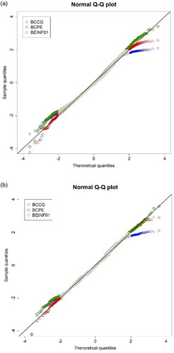
Figure 1. Q-Q plot of the normalized residuals (z-scores), derived from modeling PRC against age using three distribution families in (A) boys (n = 3,321; top panel) and (B) girls (n = 3,081; bottom panel).

Legend: the shaded area from -2 to +2 z-scores represents the range that z-scores derived from each distribution are similar.

Model selection

Building on previous knowledge of the clinical significance of age in identifying developmental delay, we first considered the statistical significance of age in the models, then we selected the most parsimonious model in terms of deviance and GAIC. Table 1 summarizes the different models tested. The minimum values for the deviance and the GAIC, for every distribution family are shown with bold fonts while the final selected model from each family is framed within a box (Table 1). These are M1.3 form BCCG, for boys and girls, that suggests that $\mu$ for PRC is best modeled using age with a smoothed function, $\sigma \mathrm{ }$ is constant (i.e. not age-dependent) whilst $\lambda \mathrm{ }$ is best modeled using a linear term for age; M2.6 for boys and M2.8 for girls from the BCPE, that suggests that $\mu$ and $\sigma \mathrm{ }$ are best modeled using age with a smoothed function, $\lambda \mathrm{ }$ using a linear term for age, whilst kurtosis is constant in boys and best modeled using a linear term for age in girls; and M3.3 for boys and M3.1 for girls from the BEINF01 that suggests that $\mu$ is best modeled using age with a smoothed function, $\sigma \mathrm{ }$ and $\lambda \mathrm{ }$ are not age-dependent, whilst kurtosis is best modeled with a linear term for age in boys but is constant in girls.

Coefficients of selected models

In all tested distribution families, there was a significant, albeit small, increase in the expected median PRC score for each day increase in age (Table S2, OLS). For example, using model M2.6, PRC in boys was expected to increase on average by 0.19 points for every additional day in participant’s age, plus the contribution of the age spline. This daily increase corresponded on average to approximately 6 points per month, plus the contribution of the age spline. Similarly, using model M3.3, the proportion of answers for which a boy received a score of 1 is expected to increase by 0.30% per daily increase in age, which is equivalent to a monthly increase of 9% on average, plus the contribution of age spline.

Diagnostic plots

The residuals were random for all three models, in boys and girls, with no clear pattern and a constant scatter against the fitted values (Figures S2 and S3, OLS) and age (Figures S4 and S5, OLS), although in models M1.3 and M2.6 for boys the residuals were not symmetrically distributed beyond the [−2, +2] range. The fitted frequency distribution for boys in models M1.3 and M2.6 had a longer left tail compared to the one fitted in M3.3 which was more symmetrical (Figure 1A; Figure S6, OLS), also showing a similar pattern in girls (Figure 1B; Figure S7, OLS). The worm plot indicated that the mixed distribution fitted the data better than the continuous distributions, mainly addressing the ceiling effect, although in the 24 mo age group the lower empirical quantile was above the theoretical with larger differences in boys compared to girls (Figures S8 and S9, OLS). Finally, as shown in Figures 2 and 3, a better approximation of the shape of the PRC distribution was achieved with the BEINF01 model and was therefore preferred against the BCPE model (Figures 2 and 3).

Figure 2. Density distributions of the total PRC score (upper left) and the fitted BCPE (lower left) and BEINF01 (lower right) distributions, using the fitted parameters of the best-selected models (BCPE, M2.6: mu = 90.22, sigma = 0.3711, lambda = 1.0512, tau = 5.3556 at the 0–158 range; BEINF01, M3.3: mu = 0.5664, sigma = 0.4284, lambda = 8.9e-09, tau = 0.0006 at the 0–1 range), in boys (n = 3,321).

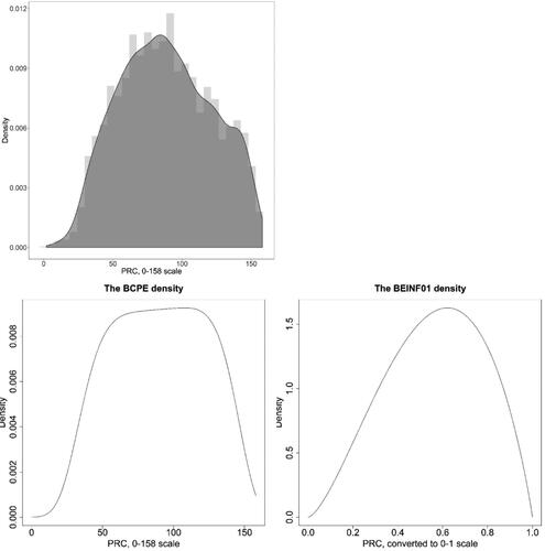
Figure 3. Density distributions of the total PRC score (upper left) and the fitted BCPE (lower left) and BEINF01 (lower right) distributions, using the fitted parameters of the best-selected models (BCPE, M2.8: mu = 108.4, sigma = 0.2774, nu = 1.733, tau = 10.50 at the 0–158 range; BEINF01, M3.1: mu = 0.6606, sigma = 0.4261, lambda = 3.3e-09, tau = 0.0033 at the 0–1 range), in girls (n = 3,081).

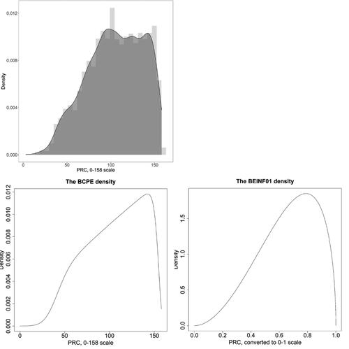
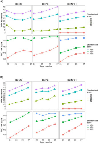
Figure 4. Trends between the standardized and PRC scores for each distribution family over age for (A) boys (n = 3,321; upper panel), and (B) girls (n = 3,081; lower panel).

Derived normalized residuals (z-scores) and centiles

Normalized residuals extracted from models M3.3 using the Beta inflated distribution were symmetrically distributed, ranging from approximately −3.9 to 3.5 in boys and −4.2 to 4.0 in girls, with mean (SD) approximating 0 (1), whilst the residuals extracted from the continuous distributions show a longer left tail in both cases (Table 2).

The sample percentages at or below specified centile curves for the fitted models against the expected percentiles are summarized in Table S3. Among the three models investigated, the BCPE model (M2.6 in boys and M2.8 in girls) performed best, especially in the lowest centiles. For the rest of the centiles, all models had similarly good fit as the sample percentages below each centile curve were close to the expected centile percentages (Table S3). The fit on the centiles affected the standardized scores, showing some small discrepancies between the expected and the calculated standardized scores for both distribution families, with the BCPE distribution showing a better fit in the lowest centiles and the Beta inflated distribution showing a better fit in the highest centiles (Table S4).

Table 3. Predicted vs raw PRC scores, by age group, using the best selected model from each distribution family, in boys (n = 3,321) and girls (n = 3,081).

	Raw PRC score
	Sample	Predicted
		BCCG	BCPE	BEINF01
Boys		M1.3	M2.6	M3.3
Age group, months
23 mo 16 d to 24 mo 15d	84 (33)	81 (32)	84 (34)	84 (36)
24 mo 16 d to 25 mo 15d	89 (33)	88 (34)	90 (33)	90 (39)
25 mo 16 d to 26 mo 15d	93 (33)	92 (36)	95 (33)	94 (40)
26 mo 16 d to 27 mo 15d	93 (34)	95 (37)	101 (32)	96 (41)
Girls		M1.3	M2.8	M3.1
Age group, months
23 mo 16 d to 24 mo 15d	102 (32)	90 (50)	105 (31)	100 (43)
24 mo 16 d to 25 mo 15d	105 (31)	93 (53)	109 (30)	105 (45)
25 mo 16 d to 26 mo 15d	109 (32)	97 (55)	114 (29)	110 (47)
26 mo 16 d to 27 mo 15d	113 (32)	102 (57)	119 (27)	115 (49)

Predicted scores were calculated using the mid-point of each age group, i.e. at 24 (i.e. 730 days), 25 (i.e. 760 days), 26 (i.e. 790 days) and 27 months (i.e. 822 days) respectively.

Predicted median values and standardized scores

For each distribution, the predicted PRC values for μ were calculated using data shown in Table S2 and plotted against age (Figures S10 and S11, OLS). Model M1.3, in boys, provided the lowest estimates across the whole age range, while M2.6 and M3.3 provided similar estimates for PRC up to the age of 25 months (approx. 760 days). Then, using M2.6, the estimates increased constantly whilst using model M3.3 PRC increased at a slower rate up to the age of 26 months (approx. 790 days) when it reached a plateau up to the age of 27 months (820 days) (Figure S10, OLS). This pattern, also evidenced in Figure S1(B) (OLS), was captured from model M3.3 with predicted PRC scores being closer to the sample average in each age group, while estimates from the BCPE overestimated the average, especially in the older age group (Table 3, top). In girls, there is a constant increase in PRC over age (Figure S2(B), OLS), which was also captured from all three distributions with lower estimates provided by the BCCG distribution and higher estimates by the BCPE distribution (Figure S11, OLS). Predicted mean PRC scores were closer to the observed data when derived from the mixed distribution (Table 3, bottom).

Figure 4 illustrates the lowest and highest standardized scores, separately for boys (A) and girls (B) by age group and their PRC equivalent for each distribution. The monotonic increase in the value of the PRC scores across the centiles was not evident when modeling the data with the BCCG distribution in boys, but this pattern was improved using the BCPE distribution. However, neither the BCCG nor the BCPE produced standardized scores that were equivalent to 3SDs (i.e. equal to a score of 145) above the mean, as could be achieved with the use of the inflated distribution. In girls, both the BCCG and the BEINF yielded monotonically increasing standard scores over age, whilst the BEINF provided standard scores equivalent to approx. 2.5SDs Moreover, only the Beta inflated at 0 and 1 distribution provided standardized scores for a PRC equal to 0 (Figure 3).

Misclassification due to inappropriate use of standardized scores

In clinical practice a standard score <70 is used to identify the 5% of a population that is at risk. Inappropriate use of cutoff points will under- or over- estimate the proportion of children at risk as we demonstrate in Table S5. For example, a raw PRC score of 30, equivalent to a standard score of 69 derived from the BCCG distribution in girls aged 24-months-old, can be used to identify 24-month-old girls at risk of developmental delay. The proportion of girls at risk will drop to 3.1%, 2.0% and 1.2% if the same cutoff point is used to identify girls at risk at 25, 26, and 27 months of age respectively. A similar drop in the proportion of children at risk using inappropriate cutoffs is observed when using the BCPE or the BINF distribution (Table S5). Underestimation of the proportion at risk is similar in boys when using the cutoffs derived from the BCPE or the BEINF, however inappropriate use of cutoffs derived from BCCG will lead to over-estimation of the population at risk (Table S5).

Discussion

This paper presents a method that, in the best of our knowledge, was applied for the first time to construct reference scores and centile curves for assessing children’s cognitive and language development. It also highlights limitations that may occur when inappropriate distributions are used to extract the centiles, whilst modeling the already known association of developmental test scores with age. Here we provide a guide for the different steps one need to follow for producing standardized scores that could also be applicable in other settings (e.g. for blood pressure or other cognitive tests).

In order to produce the PARCA-R standardized scores with the PRC score as the response variable, three distribution families were examined and compared in terms of their ability to produce correct fitted centiles: the Box-Cox-Cole-Green (equivalent to the common LMS method), the Box-Cox-Power-Exponential and the Beta inflated at [0, 1] distributions. The results indicated that the Beta inflated at [0, 1] distribution was the most appropriate to construct reference scores across the whole range and to address the ceiling effect that is present when a measurement tool is bounded in a certain range.

For constructing the reference scores, one needs to consider the distribution family to be selected, the smoothing functions of the explanatory variable(s) and the link function of the response variable. As we were interested in generating age-specific reference scores, age was the only explanatory variable that was used in the modeling. Depending on the distribution family, age might be significant in different parameters of the response variable distribution and this affects the predicted values. For example, in our case, age was significant when predicting the scale parameter (sigma, $\sigma$) using the BCPE distribution, while it was significant when predicting skewness (lambda, $\lambda$) using the BCCG and the BCPE distributions. Therefore, it is important to recognize that two equivalent models may produce different predicted scores. In addition, the smoothing function for age may not be required in all the distribution parameters. In our analysis, using a smoothing function for age to model skewness and kurtosis in the continuous distributions led to an over-smoothed model that subsequently resulted in biased centile curves, as indicated by the unexpected pattern of the standardized scores as age increased and their non-plausible range (i.e. standardized scores that ranged from −3 to 140). Therefore, it was inappropriate to model skewness and kurtosis with smoothing terms. With respect to the link functions, we used the default link function for the response outcome in all the distribution parameters, as indicated in Table S2 (OLS), and did not apply any transformation on the explanatory variable as their association was linear and variability was quite constant across the age range. In addition, all children in our sample had PRC > 0, so either distribution family worked well with the modeling. However, if PRC equals 0 a constant term should be added to that value or this should be excluded in order to apply the continuous distributions. The BEINF01 is the only distribution that allows modeling of the whole range of the scale and thus obtaining standardized scores for 0.

The two main distribution families were not directly comparable, as the response variable was in the raw scale (0, 158] when using the continuous distributions and in a transformed [0, 1] scale when using the mixed distribution. Nevertheless, we used the proportion of answers for which a child could score 1 for as the response variable (similar to what we did when applying the beta-inflated model) for the BCCG and BCPE models. This did not affect model selection for the continuous distributions and produced similar z-scores, and thus similar predicted and standardized scores, to the ones extracted using the 0–158 scale as the response variable. Therefore, results were presented only on the raw scale for the BCCG and BCPE models.

The GAMLSS (Rigby & Stasinopoulos, 2005) offers a wide selection of distributions for modeling the response variable, also including distributions from the discrete family. Considering PRC as a discrete scale, we also examined whether a distribution of the discrete family of distributions could fit the data better. However, neither of the distributions tested (i.e. the Poisson inverse Gaussian, the beta negative binomial, the Delaporte and the zero inflated negative binomial distributions) resulted in normally distributed residuals nor addressed the ceiling effect, therefore were not considered for presentation. It has also been suggested that a Tobit model based on the Student-t distribution could be used to replace the beta distribution, which often has a poor fit to a proportion response variable on (0, 1) in real datasets (Hossain et al., 2016). This distribution, tested in our data, also failed to fulfill the assumptions of normality of the standardized residuals, as evidenced from the diagnostic plots, and also produced an excess concentration of values around +2SDs from the mean and therefore was not preferred against the beta-inflated distribution at [0, 1].

The application of quantile regression (Koenker, 2017) could have been an alternative approach for estimating age-specific reference scores, especially when the assumptions of linear models (i.e. linearity, homoscedasticity, normality) are not met. Quantile regression allows the calculation of any percentile for a particular value of the predictor(s). Therefore, it would have been useful to calculate, for example, the 5th percentile for the PRC score at a particular age, meaning that there is a 5% chance the actual PRC score is below the prediction for that particular age. Although the quantile regression is useful to rank individuals of a specific sample according to their scores, it avoids making distributional assumptions and, as such, cannot provide z-scores, which are useful for quantifying measurements on a continuous scale and for clinical decision making (van Buuren, 2007), or making the scale comparable to other developmental tests. Regardless, we applied quantile regression in our data but computational problems occurred due to the presence of many ties that precluded the estimation of the fitted centiles.

Similar to monitoring growth problems, developmental delay is more efficient and cost-effective when detected early to allow for early instigation of intervention (Black et al., 2017). To assess developmental delay a child’s score is compared against that of children of a similar age and a decision to refer the child for clinical assessment of intervention is then made (Bellman et al., 2013). It is therefore important to ensure that appropriate standards are used when generating standardized scores to avoid over- or under-referrals. Ignoring age-related changes in the scale and/or the location parameters of the distribution of the response variable will derive either too low or too high z-scores, which result in biased centiles and may mislead clinicians as to the child’s true developmental level (Royston & Wright, 1998, 2000). Although in our data, using the beta inflated distribution 2.5% of the cases were below the 4.5^th centile and 5% below the 7^th centile, the z-scores calculated from the predicted values corresponded to the 2.45^th centile for 2.5% of the cases and 4.8^th centile for 5% of the cases which confirmed the suitability of the equations for the extraction of the standardized scores.

It is acknowledged that emphasis should be given to accurately capturing the lower centiles to identify children at risk of delay; however, the use of a distribution that does not handle the ceiling effect properly is also problematic. Ceiling effects occur when a test is relatively easy, so participants can reach the highest possible score and cannot demonstrate the true extent of their abilities (Garin, 2014). In the presence of a ceiling effect, the variability among individuals is underestimated and the true score range is reduced so differences among high-scorers are not evident, leading to biased derived scores (Uttl, 2005; Wang et al., 2008). The use of the beta-inflated distribution addressed this limitation and produced symmetrically distributed z-scores beyond ±3SDs of the mean.

In clinical practice, the decision to refer a child for intervention is based on age-specific centile curves. An individual’s score or measurement is related to a distribution from an age-specific reference group and this comparison gives an indication of the position of the individual relative to the reference group at that age. These centiles are commonly constructed using the LMS method. However, we advise that one should inspect the underlying distribution and select the appropriate transformation for constructing the centiles, rather than applying the LMS by default which may end up over- or under- estimating the people at risk and in need of intervention. Inaccurate centiles may mislead the clinician as to the true developmental level of the child and may increase the chance of under- or over-referral. Therefore, the appropriate selection of the distribution family to model the response measurement against age and to construct these centile curves is crucial.

Article information

Conflict of interest disclosures: Each author signed a form for disclosure of potential conflicts of interest. No authors reported any financial or other conflicts of interest in relation to the work described. Contributors: VB analyzed and interpreted the data, wrote the first draft of the manuscript, critically reviewed and revised the manuscript for important intellectual content, and approved the final version for submission; SJ contributed to the study design and analysis strategy, critically reviewed and revised the manuscript for important intellectual content, and approved the final version for submission; BM contributed to the study design and analysis strategy, critically reviewed and revised the manuscript for important intellectual content, and approved the final version for submission.

Ethical principles: The authors affirm having followed professional ethical guidelines in preparing this work. These guidelines include obtaining informed consent from human participants, maintaining ethical treatment and respect for the rights of human or animal participants, and ensuring the privacy of participants and their data, such as ensuring that individual participants cannot be identified in reported results or from publicly available original or archival data.

Funding: This work was supported by Grant GN2580 from the Action Medical Research Project, awarded to Samantha Johnson and Bradley Manktelow (University of Leicester), Louise Linsell (University of Oxford), Peter Brocklehurst (University of Birmingham), Dieter Wolke (University of Warwick) and Neil Marlow (University College London).

Role of the funders/sponsors: None of the funders or sponsors of this research had any role in the design and conduct of the study; collection, management, analysis, and interpretation of data; preparation, review, or approval of the manuscript; or decision to submit the manuscript for publication.

Acknowledgments: The authors are grateful to all the parents who took part in the INFANT, LAMBS and PANDA studies. The authors would also like to express their gratitude to Dr Louise Linsell, Principal Statistician at Visible Analytics, for her valuable comments and suggestions whilst drafting the earlier versions of this manuscript. The ideas and opinions expressed herein are those of the authors alone, and endorsement by the authors’ institutions or the funding agency is not intended and should not be inferred.

Data availability statement

Data sharing is not applicable as secondary data were analyzed in this study, hence no new data were created in this study. The code used to analyze the current data is available as an Appendix in the online supplementary material. The parameters obtained from the equations derived from the mixed distributions are also freely available on the PARCA-R website (www.parca-r.info) to facilitate its use in research and clinical practice.

References

- Abbott, J., Berrington, J., Bowler, U., Boyle, E., Dorling, J., Embleton, N., Juszczak, E., Leaf, A., Linsell, L., Johnson, S., McCormick, K., McGuire, W., Roberts, T., & Stenson, B, Sift Investigators Group. (2017). The speed of increasing milk feeds: A randomised controlled trial. BMC Pediatrics, 17(1), 39. https://doi.org/10.1186/s12887-017-0794-z.
- Adani, S., & Cepanec, M. (2019). Sex differences in early communication development: Behavioral and neurobiological indicators of more vulnerable communication system development in boys. Croatian Medical Journal, 60(2), 141–149. https://doi.org/10.3325/cmj.2019.60.141.
- Akaike, H. (1983). Information measures and model selection. Bulletin of the International Statistical Institute, 50, 277–290.
- American Academy of Pediatrics. (2001). Committee on children with disabilities. developmental surveillance and screening of infants and young children. http://pediatrics.aappublications.org/content/pediatrics/108/1/192.full.pdf
- Bayley, N. (2006). Bayley scales of infant and toddler development. (H. A. Inc Ed. 3rd ed.) TX.
- Beardmore-Gray, A., Greenland, M., Linsell, L., Juszczak, E., Hardy, P., Placzek, A., … Chappell, L. C. (2022). Two-year follow-up of infant and maternal outcomes after planned early delivery or expectant management for late preterm pre-eclampsia (PHOENIX): A randomised controlled trial. British Journal of Obstetrics and Gynaecology, 129(10), 1654–1663. https://doi.org/10.1111/1471-0528.17167
- Bellman, M., Byrne, O., & Sege, R. (2013). Developmental assessment of children. BMJ, 346(jan15 2), e8687–e8687. https://doi.org/10.1136/bmj.e8687
- Black, M. M., Walker, S. P., Fernald, L. C. H., Andersen, C. T., DiGirolamo, A. M., Lu, C., McCoy, D. C., Fink, G., Shawar, Y. R., Shiffman, J., Devercelli, A. E., Wodon, Q. T., Vargas-Barón, E., … Grantham-McGregor, S. (2017). Early childhood development coming of age: Science through the life course. Lancet (London, England), 389(10064), 77–90. https://doi.org/10.1016/S0140-6736(16)31389-7
- Blaggan, S., Guy, A., Boyle, E. M., Spata, E., Manktelow, B. N., Wolke, D., & Johnson, S. (2014). A parent questionnaire for developmental screening in infants born late and moderately preterm. Pediatrics, 134(1), E55–E62. https://doi.org/10.1542/peds.2014-0266.
- Box, G. E. P., & Cox, D. R. (1964). An analysis of transformations. Journal of the Royal Statistical Society. Series B (Methodological), 26(2), 211–243. https://doi.org/10.1111/j.2517-6161.1964.tb00553.x
- Boyle, E. M., Johnson, S., Manktelow, B., Seaton, S. E., Draper, E. S., Smith, L. K., Dorling, J., Marlow, N., Petrou, S., & Field, D. J. (2015). Neonatal outcomes and delivery of care for infants born late preterm or moderately preterm: A prospective population-based study. Archives of Disease in Childhood. Fetal and Neonatal Edition, 100(6), F479–F485. https://doi.org/10.1136/archdischild-2014-307347.
- Brocklehurst, P., Farrell, B., King, A., Juszczak, E., Darlow, B., Haque, K., Salt, A., Stenson, B., & Tarnow-Mordi, W, INIS Collaborative Group (2011). Treatment of neonatal sepsis with intravenous immune globulin. The New England Journal of Medicine, 365(13), 1201–1211. https://doi.org/10.1056/NEJMoa1100441.
- Brooks, B. L., Sherman, E. M. S., & Strauss, E. (2009). NEPSY-II: A developmental neuropsychological assessment, second edition. Child Neuropsychology, 16(1), 80–101. https://doi.org/10.1080/09297040903146966
- Cole, T. J., & Green, P. J. (1992). Smoothing reference centile curves: The LMS method and penalized likelihood. Statistics in Medicine, 11(10), 1305–1319. https://doi.org/10.1002/sim.4780111005.
- Cole, T. J., Stanojevic, S., Stocks, J., Coates, A. L., Hankinson, J. L., & Wade, A. M. (2009). Age- and size-related reference ranges: A case study of spirometry through childhood and adulthood. Statistics in Medicine, 28(5), 880–898. https://doi.org/10.1002/sim.3504.
- Cuttini, M., Ferrante, P., Mirante, N., Chiandotto, V., Fertz, M., Dall’Oglio, A. M., Coletti, M. F., & Johnson, S. (2012). Cognitive assessment of very preterm infants at 2-year corrected age: Performance of the Italian version of the PARCA-R parent questionnaire. Early Human Development, 88(3), 159–163. https://doi.org/10.1016/j.earlhumdev.2011.07.022.
- Dean, K., Walker, Z., & Jenkinson, C. (2018). Data quality, floor and ceiling effects, and test-retest reliability of the Mild Cognitive Impairment Questionnaire. Patient Related Outcome Measures, 9, 43–47. https://doi.org/10.2147/PROM.S145676.
- Department for Communities and Local Government (2011). The English Indices of Deprivation 2010.
- Dorling, J., Abbott, J., Berrington, J., Bosiak, B., Bowler, U., Boyle, E., Embleton, N., Hewer, O., Johnson, S., Juszczak, E., Leaf, A., Linsell, L., McCormick, K., McGuire, W., Omar, O., Partlett, C., Patel, M., Roberts, T., Stenson, B., & Townend, J, for the SIFT Investigators Group. (2019). Controlled trial of two incremental milk feeding rates in preterm infants. The New England Journal of Medicine, 381(15), 1434–1443. https://doi.org/10.1056/NEJMoa1816654.
- Draper, E. S., Zeitlin, J., Manktelow, B. N., Piedvache, A., Cuttini, M., Edstedt Bonamy, A.-K., Maier, R., Koopman-Esseboom, C., Gadzinowski, J., Boerch, K., van Reempts, P., Varendi, H., & Johnson, S. J, EPICE group (2020). EPICE Cohort: Two year neurodevelopmental outcomes after very preterm birth. Archives of Disease in Childhood. Fetal and Neonatal Edition, 105(4), 350–356. https://doi.org/10.1136/archdischild-2019-317418.
- Eilers, P. H. C., & Marx, B. D. (1996). Flexible smoothing with B-splines and penalties. Statistical Science, 11(2), 89–102. https://doi.org/10.1214/ss/1038425655
- Engle, P. L., Fernald, L. C. H., Alderman, H., Behrman, J., O'Gara, C., Yousafzai, A., de Mello, M. C., Hidrobo, M., Ulkuer, N., Ertem, I., … Iltus, S, Global Child Development Steering (2011). Strategies for reducing inequalities and improving developmental outcomes for young children in low-income and middle-income countries. Lancet (London, England), 378(9799), 1339–1353., G https://doi.org/10.1016/S0140-6736(11)60889-1
- European Foundation for the Care of Newborn Infants (EFCNI) (2018). European Standards of Care for Newborn Health. https://newborn-health-standards.org/project/about-2/.
- Field, D., Spata, E., Davies, T., Manktelow, B., Johnson, S., Boyle, E., & Draper, E. S. (2016). Evaluation of the use of a parent questionnaire to provide later health status data: The PANDA study. Archives of Disease in Childhood. Fetal and Neonatal Edition, 101(4), F304–F308. https://doi.org/10.1136/archdischild-2015-309247.
- Garin, O. (2014). Ceiling Effect. In A. C. Michalos (Ed.), Encyclopedia of quality of life and well-being research (pp. 631–633). Springer Netherlands.
- Gluhm, S., Goldstein, J., Loc, K., Colt, A., Van Liew, C., & Corey-Bloom, J. (2013). Cognitive Performance on the Mini-Mental State Examination and the Montreal Cognitive Assessment Across the Healthy Adult Lifespan. Cognitive and Behavioral Neurology: Official Journal of the Society for Behavioral and Cognitive Neurology, 26(1), 1–5. https://doi.org/10.1097/WNN.0b013e31828b7d26.
- Gupta, S., Juszczak, E., Hardy, P., Subhedar, N., Wyllie, J., Kelsall, W., Sinha, S., Johnson, S., Roberts, T., Hutchison, E., Pepperell, J., Linsell, L., Bell, J. L., Stanbury, K., Laube, M., Edwards, C., …, & Field, D, Field D on behalf of The Baby-OSCAR Collaborative Group (2021). Study protocol: Baby-OSCAR trial: Outcome after Selective early treatment for Closure of patent ductus Arteriosus in preterm babies, a multicentre, masked, randomised placebo-controlled parallel group trial. BMC Pediatrics, 21(1), 100. https://doi.org/10.1186/s12887-021-02558-7
- Hayat, S. A., Luben, R., Moore, S., Dalzell, N., Bhaniani, A., Anuj, S., Matthews, F. E., Wareham, N., Khaw, K.-T., & Brayne, C. (2014). Cognitive function in a general population of men and women: A cross sectional study in the European Investigation of Cancer–Norfolk cohort (EPIC-Norfolk). BMC Geriatrics, 14, 142. https://doi.org/10.1186/1471-2318-14-142.
- Hossain, A., Rigby, R., Stasinopoulos, M., & Enea, M. (2016). Centile estimation for a proportion response variable. Statistics in Medicine, 35(6), 895–904. https://doi.org/10.1002/sim.6748.
- Infant Collaborative Group (2017). Computerised interpretation of fetal heart rate during labour (INFANT): A randomised controlled trial. Lancet, 389(10080), 1719–1729. https://doi.org/10.1016/S0140-6736(17)30568-8
- International Consortium for Health Outcomes Measurement (ICHOM) (2020)., Preterm and Hospitalized Newborn Health Group, NEO Standard Set Retrieved from https://www.ichom.org/portfolio/preterm-and-hospitalized-newborn-health/).
- Johnson, S., Marlow, N., Wolke, D., Davidson, L., Marston, L., O'Hare, A., Peacock, J., & Schulte, J. (2004). Validation of a parent report measure of cognitive development in very preterm infants. Developmental Medicine and Child Neurology, 46(6), 389–397. https://doi.org/10.1017/S0012162204000635.
- Johnson, S., Wolke, D., & Marlow, N, Preterm Infant Parenting Study Group (2008). Developmental assessment of preterm infants at 2 years: Validity of parent reports. Developmental Medicine and Child Neurology, 50(1), 58–62. https://doi.org/10.1111/j.1469-8749.2007.02010.x
- Johnson, S., Evans, T. A., Draper, E. S., Field, D. J., Manktelow, B. N., Marlow, N., Matthews, R., Petrou, S., Seaton, S. E., Smith, L. K., & Boyle, E. M. (2015). Neurodevelopmental outcomes following late and moderate prematurity: A population-based cohort study. Archives of Disease in Childhood. Fetal and Neonatal Edition, 100(4), F301–8. https://doi.org/10.1136/archdischild-2014-307684
- Johnson, S., Bountziouka, V., Brocklehurst, P., Linsell, L., Marlow, N., Wolke, D., & Manktelow, B. N. (2019). Standardisation of the Parent Report of Children’s Abilities-Revised (PARCA-R): A norm-referenced assessment of cognitive and language development at age 2 years. The Lancet Child Adolescent Health, 3(1), 709–712. https://doi.org/10.1016/S2352-4642(19)30189-0
- Kobayashi, T., Fuse, S., Sakamoto, N., Mikami, M., Ogawa, S., Hamaoka, K., Arakaki, Y., Nakamura, T., Nagasawa, H., Kato, T., Jibiki, T., Iwashima, S., Yamakawa, M., Ohkubo, T., Shimoyama, S., Aso, K., Sato, S., … Saji, T, Investigators (2016). A New Z Score Curve of the Coronary Arterial Internal Diameter Using the Lambda-Mu-Sigma Method in a Pediatric Population. Journal of the American Society of Echocardiography: Official Publication of the American Society of Echocardiography, 29(8), 794–801.e29., Z. S. P. https://doi.org/10.1016/j.echo.2016.03.017.
- Koenker, R. (2017). Quantile regression: 40 years on. Annual Review of Economics, 9(1), 155–176. https://doi.org/10.1146/annurev-economics-063016-103651
- Marino, B. S., Lipkin, P. H., Newburger, J. W., Peacock, G., Gerdes, M., Gaynor, J. W., Mussatto, K. A., Uzark, K., Goldberg, C. S., Johnson, W. H., Li, J., Smith, S. E., Bellinger, D. C., & Mahle, W. T, American Heart Association Congenital Heart Defects Committee, Council on Cardiovascular Disease in the Young, Council on Cardiovascular Nursing, and Stroke Council. (2012). Neurodevelopmental outcomes in children with congenital heart disease: Evaluation and management: A scientific statement from the American Heart Association. Circulation, 126(9), 1143–1172. https://doi.org/10.1161/CIR.0b013e318265ee8a.
- Marlow, N., Greenough, A., Peacock, J. L., Marston, L., Limb, E. S., Johnson, A. H., & Calvert, S. A. (2006). Randomised trial of high frequency oscillatory ventilation or conventional ventilation in babies of gestational age 28 weeks or less: Respiratory and neurological outcomes at 2 years. Archives of Disease in Childhood. Fetal and Neonatal Edition, 91(5), F320–326. https://doi.org/10.1136/adc.2005.079632.
- Martin, A. J., Darlow, B. A., Salt, A., Hague, W., Sebastian, L., Mann, K., & Tarnow-Mordi, W, Inis Trial Collaborative Group (2012). Identification of infants with major cognitive delay using parental report. Developmental Medicine and Child Neurology, 54(3), 254–259. https://doi.org/10.1111/j.1469-8749.2011.04161.x.
- Martin, A. J., Darlow, B. A., Salt, A., Hague, W., Sebastian, L., McNeill, N., & Tarnow-Mordi, W. (2013). Performance of the Parent Report of Children’s Abilities Revised (PARCA-R) versus the Bayley Scales of Infant Development III. Archives of Disease in Childhood, 98(12), 955–958. https://doi.org/10.1136/archdischild-2012-303288.
- Muniz-Terrera, G., Hout, A., Rigby, R. A., & Stasinopoulos, D. M. (2016). Analysing cognitive test data: Distributions and non-parametric random effects. Statistical Methods in Medical Research, 25(2), 741–753. https://doi.org/10.1177/0962280212465500.
- NICE Guideline: Developmental follow-up of children and young people born preterm. (2017). Retrieved from www.nice.org.uk/guidance/ng72.
- Norris, T., Seaton, S. E., Manktelow, B. N., Baker, P. N., Kurinczuk, J. J., Field, D., Draper, E. S., & Smith, L. K. (2018). Updated birth weight centiles for England and Wales. Archives of Disease in Childhood. Fetal and Neonatal Edition, 103(6), F577–F582. https://doi.org/10.1136/archdischild-2017-313452
- Picotti, E., Bechtel, N., Latal, B., Borradori-Tolsa, C., Bickle-Graz, M., Grunt, S., Johnson, S., Wolke, D., & Natalucci, G, Swiss Neonatal Network & Follow-Up Group. (2020). Performance of the German version of the PARCA-R questionnaire as a developmental screening tool in two-year-old very preterm infants. PloS One, 15(9), e0236289. https://doi.org/10.1371/journal.pone.0236289.
- Quanjer, P. H., Stanojevic, S., Cole, T. J., Baur, X., Hall, G. L., Culver, B. H., Enright, P. L., Hankinson, J. L., Ip, M. S. M., Zheng, J., & Stocks, J, ERS Global Lung Function Initiative (2012). Multi-ethnic reference values for spirometry for the 3–95-yr age range: The global lung function 2012 equations. The European Respiratory Journal, 40(6), 1324–1343. https://doi.org/10.1183/09031936.00080312.
- R Core Team (2017). R: A language and environment for statistical computing. Austria. R Foundation for Statistical Computing. Retrieved from https://www.R-project.org/
- Report of a BAPM/RCPCH Working Group: Classification of health status at 2 years as a perinatal outcome. (2008). https://www.networks.nhs.uk/nhs-networks/staffordshire-shropshire-and-black-country-newborn/documents/2_year_Outcome_BAPM_WG_report_v6_Jan08.pdf
- Rigby, R., & Stasinopoulos, D. (2005). Generalized additive models for location, scale and shape. Journal of the Royal Statistical Society: Series C (Applied Statistics), 54(3), 507–554. https://doi.org/10.1111/j.1467-9876.2005.00510.x
- Rigby, R., Stasinopoulos, D., Heller, G., & De Bastiani, F. (2020). Distributions for modelling location, scale, and shape: Using GAMLSS in R. CRC Press. Taylor & Francis Group.
- Rigby, R., & Stasinopoulos, M. (2004). Smooth centile curves for skew and kurtotic data modelled using the Box–Cox power exponential distribution. Statistics in Medicine, 23(19), 3053–3076. https://doi.org/10.1002/sim.1861.
- Royston, P., & Wright, E. M. (1998). How to construct 'normal ranges’ for fetal variables. Ultrasound in Obstetrics & Gynecology: The Official Journal of the International Society of Ultrasound in Obstetrics and Gynecology, 11(1), 30–38. https://doi.org/10.1046/j.1469-0705.1998.11010030.x.
- Royston, P., & Wright, E. M. (2000). Goodness-of-fit statistics for age-specific reference intervals. Statistics in Medicine, 19(21), 2943–2962. https://doi.org/10.1002/1097-0258(20001115)19:21 < 2943::aid-sim559 > 3.0.co;2-5
- Saudino, K. J., Dale, P. S., Oliver, B., Petrill, S. A., Richardson, V., Rutter, M., Simonoff, E., Stevenson, J., & Plomin, R. (1998). The validity of parent-based assessment of the cognitive abilities of 2-year-olds. British Journal of Developmental Psychology, 16(3), 349–362. https://doi.org/10.1111/j.2044-835X.1998.tb00757.x
- Schwarz, G. (1978). Estimating the dimension of a model. Ann Statist, 6, 461–464. https://doi.org/10.1214/aos/1176344136
- Uttl, B. (2005). Measurement of individual differences: Lessons from memory assessment in research and clinical practice. Psychological Science, 16(6), 460–467. https://doi.org/10.1111/j.0956-7976.2005.01557.x.
- van Buuren, S. (2007). Worm plot to diagnose fit in quantile regression. Statistical Modelling, 7(4), 363–376. https://doi.org/10.1177/1471082X0700700406
- van Buuren, S., & Fredriks, M. (2001). Worm plot: A simple diagnostic device for modelling growth reference curves. Statistics in Medicine, 20(8), 1259–1277. https://doi.org/10.1002/sim.746.
- Vanhaesebrouck, S., Theyskens, C., Vanhole, C., Allegaert, K., Naulaers, G., de Zegher, F., & Daniels, H. (2014). Cognitive assessment of very low birth weight infants using the Dutch version of the PARCA-R parent questionnaire. Early Human Development, 90(12), 897–900. https://doi.org/10.1016/j.earlhumdev.2014.10.004.
- Wang, L. J., Zhang, Z. Y., McArdle, J. J., & Salthouse, T. A. (2008). Investigating ceiling effects in longitudinal data analysis. Multivariate Behavioral Research, 43(3), 476–496. https://doi.org/10.1080/00273170802285941.
- WHO Multicentre Growth Reference Study Group. WHO Child Growth Standards: Growth velocity based on weight, length and head circumference: Methods and development (2009). Geneva: World Health Organization.
- Wickham, H. (2009). ggplot2: Elegant graphics for data analysis. Springer-Verlag.