Turbulent mixing in a stratified estuarine tidal channel: Hikapu Reach, Pelorus Sound, New Zealand

ABSTRACT

Channel constrictions within an estuary can influence overall estuary-sea exchange of salt or suspended/dissolved material. The exchange is modulated by turbulent mixing through its effect on density stratification. Here we quantify turbulent mixing in Hikapu Reach, an estuarine channel in the Marlborough Sounds, New Zealand. The focus is on a period of relatively low freshwater input but where density stratification still persists throughout the tidal cycle, although the strength of stratification and its vertical structure vary substantially. The density stratification increases through the ebb tide, and decreases through the flood tide. During the spring tides observed here, ebb tidal flow speeds reached 0.7 m s⁻¹ and the buoyancy frequency squared was in the range 10⁻⁵ to 10⁻³ s⁻². Turbulence parameters were estimated using both shear microstructure and velocimeter-derived inertial dissipation which compared favourably. The rate of dissipation of turbulent kinetic energy reached 1 × 10⁻⁶ m² s⁻³ late in the ebb tide, and estimates of the gradient Richardson number (the ratio of stability to shear) fell as low as 0.1 (i.e. unstable) although the results show that bottom-boundary driven turbulence can dominate for periods. The implication, based on scaling, is that the mixing within the channel does not homogenise the water column within a tidal cycle. Scaling, developed to characterise the tidal advection relative to the channel length, shows how riverine-driven buoyancy fluxes can pass through the tidal channel section and the stratification can remain partially intact.

KEYWORDS:

• Estuary
• Pelorus Sound
• tidal mixing
• stratification
• turbulence

Introduction

Estuaries form an interface in the hydrologic cycle between the land and the coastal ocean. Understanding the evolution of stratification in estuaries and coastal embayments is important for categorising the behaviour and timescales controlling this interface (Geyer & MacCready 2014). This underpins quantification and categorisation of factors such as overall biological productivity, ecological structuring and ultimately decisions relating to human activity including CO₂ exchange, consequences of nutrient loading through land-use and aquaculture driven eutrophication (e.g. Li et al. 2000; Zeldis et al. 2013).

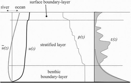
In some instances estuaries themselves are divided by some constriction in the form of an estuarine tidal channel, typically a section of estuary longer than it is wide with largely bi-directional flow. The mixing in this region is controlled by stratification, internal shear and boundary-driven mixing, and varies dramatically over timescales associated with tidal flows. Some key features are shown in Figure 1: a tidally varying velocity profile u(z,t), stratification derived from the interplay of freshwater input and seawater incursion and straining by the velocity profile. Furthermore, because the channel occurs within an estuary, the enhanced mixing acts as a controlling influence (in a general, rather than hydraulic, sense) on the estuary-wide transport and exchange processes that connect the freshwater and marine environments (Wild-Allen et al. 2013; Geyer & MacCready 2014).

Figure 1. Basic structure of a dynamic partially stratified estuary, showing: water column structure for velocity (showing both instantaneous–in this case ebb = u(z) and mean ‘estuarine circulation’ = u dotted) and density ρ with benthic and surface boundary-layers with and intermediate stratified later. The boundaries and internal shear produce turbulence which is dissipated at rate ε (the dotted line is an indicative law of the wall decay). The instantaneous velocity profile oscillates back and forth with the tidal ebb and flood generating a highly variable dissipation rate structure.

Turbulent mixing and water column modification in estuarine tidal channels are well-studied in general terms (e.g. Stacey et al. 1999; Peters 2003; Geyer & MacCready 2014), evolving as they did from the very initial observational work on ocean turbulence (Grant et al. 1962). Stratification and its persistence are intimately connected with levels of turbulent kinetic energy (e.g. Orton et al. 2010). The rate of change in turbulent kinetic energy (E_KE) is given by:(1) which is the sum of shear production (P), buoyancy flux (B), rate of turbulent dissipation ε, and additional terms (T) associated with pressure and divergence. Assuming T is small when averaged, profiled descriptions of P and ε, in conjunction with the stratification, can be used to describe diapycnal diffusion. As Peters and Bokhorst (2000) note, while the turbulent dissipation rate may not be the most interesting component, it can enable quantities such as diapycnal diffusivity to be calculated. It remains to categorically identify the relationship between dissipation and diffusion in highly stratified estuarine conditions.

Benthic boundary layer mixing is dependent on the hydraulic roughness of the bed which for present purposes can be described by a drag coefficient C_d. This can be characterised by a Law of the Wall distribution of energy dissipation rate making it possible to infer the contribution of benthic boundary mixing (u³ _*/[κz]) to the overall dissipation rate profile (κ is von Kármán’s constant, z is height above bed, and u* is a friction velocity inferred from the flow speed and a drag coefficient C_d).

Internal shear-induced mixing is encapsulated in the gradient Richardson Number representing the relative strength of stabilising stratification versus destabilising velocity shear. The gradient in density stratification is quantified using the buoyancy frequency squared comprising a reference (background) density ρ₀, gravitational acceleration g and the vertical derivative of density, . The gradient Richardson Number, represents the ratio of this stability factor to the shear, Sh_A, the vertical derivative of velocity: , so that

This provides a measure of shear-induced instability whereby values substantially less than unity are likely to be, or become, unstable. (Ri_gr = 0.25 is the theoretical value for instability and Ri_gr < 0 indicates convective instability).

Outer scales driving these combined mixing processes are the tidal flow and the imposed horizontal density gradient which is then ‘strained’ by the flow (Simpson et al. 2005) and so becomes self-sustaining. The change in potential energy due to straining relative to the production of turbulent kinetic energy by bed friction is encapsulated in the Simpson numberwhere b_x is the horizontal gradient in buoyancy (g/ρ₀)(dρ/dx), H is the water depth, C_d the benthic drag coefficient and U_T is the amplitude of the depth-averaged tidal velocity. For small Si, tidally induced mixing dominates and the water column is vertically well-mixed. Conversely, large Si indicates that tidal straining may be sufficient to maintain stratification through the tidal cycle as strain induces a continued vertical density gradient. However, Si does not explicitly include a time-scale nor the effect of internal shear. The duration of the ebb or flood tidal flow relative to the time for turbulent entrainment of the water column is an additional mixing parameter and is represented bywhere ω is the tidal angular frequency and N₀ is an average buoyancy frequency (Geyer & MacCready 2014). A small value for M, say <1, indicates that mixing cannot penetrate the entire depth in one-half of a tidal cycle.

The field site considered here, Hikapu Reach, is well-suited for examining details of the balance of stratification and shear as it exhibits a modest range of stratification stabilities and is reasonably strongly tidally-forced. In terms of comparable studies (Table 1), it is one of the deeper channels. The objectives of the present study are to (i) place the Hikapu Reach results in the context of available paradigms for estuarine mixing, (ii) use and compare two measurement techniques to quantify the variability and structure of the turbulence as a function of tidal phase, (iii) compare the balance of internal shear versus bed-driven turbulence and (iv) identify implications for exchange and dilution in estuarine systems.

Table 1. Tidal channel bulk parameters as estimated from various studies.

Location	Method	Umax m s^−1	H m	N^2 s^−2	Sh^2 s^−2	Lc Km	Cr
Hikapu Reach, NZ this study	S,T,V	0.75	34	5 × 10^−4	5 × 10^−5	4	4.2
Cordova Chan, Canada^1	H	0.85	30	–	4 × 10^−5	3	6.3
Hopkins River, Vic. Australia^2	T	0.25	5	0.2	0.06	9	0.6
Hudson (Cassie), USA^3	V, A	0.5	5	0.002	0.015	45–110	0.2
Hudson River USA^4	S	1.0	15	0.005	0.01	45–110	0.3
Meeker Slough, USA^5	V	0.35	2	0.3	0.01	c. 1	7.8
Menai Strait, Wales, UK^6	A	1.3	15	–	0.025	20	1.5
Merrimack estuary, USA^7	V	0.8	6	0.03	0.015	10	1.8
Suisun Cutoff, USA^8	A	0.75	10–12	0.01	0.01	2	8.4
Swan River, Australia^9	T	0.7	4	0.004	0.001	30	0.5
York River, USA^10	A	1.0	6	–	–	40	0.6

The sampling methods are vertical shear profiler SMS (S), horizontal shear (H), temperature gradient microstructure (T), ADCP variance (A) and velocimeter IDM (V) approaches. The channel length L_c either represents the full estuary extent or a particular section length if that is identifiable (¹Lu et al. 2000; ²Sharples et al. 2003; ³Orton et al. 2010; ⁴Peters 2003; ⁵Ralston & Stacey 2007; ⁶Rippeth et al. 2002; ⁷Geyer et al. 2008; ⁸Stacey et al. 1999; ⁹O’Callaghan et al. 2010; ¹⁰Simpson et al. 2005.)

Location and methods

Location

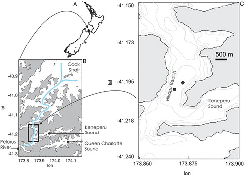
Observations of currents, stratification and turbulence were recorded in Hikapu Reach (41.20S 173.87E), a 4 km long, relatively straight section of Pelorus Sound, New Zealand (Figure 2). The sound is one of the two main waterways comprising the Marlborough Sounds area at the northern end of South Island, New Zealand (Figure 2), the other being Queen Charlotte Sound. Pelorus Sound is formed by a drowned sequence of mountain ranges and so forms a sinuous main channel, ca 55 km long, with several major side arms and many embayments (Heath 1976; Sutton & Hadfield 1997; Stevens 2003, 2010).

Figure 2. Map showing A, New Zealand; B, Pelorus Sound and its main channel (blue), the Pelorus River, the large inlet of Keneperu Sound and the adjacent but unconnected Queen Charlotte Sound. C, Shows the study site Hikapu Reach, where the grey lines are 10 m contours. The square is the RDCP/Vector mooring and the diamond is the approximate location of the profiling vessel although this would move on its mooring.

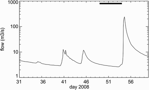
The Sound undergoes an annual cycle in water column structure whereby temperature influences on density are typically dominated by salinity stratification (Sutton & Hadfield 1997). A key difference between Pelorus Sound and the neighbouring Queen Charlotte Sound is the presence of the freshwater inflow into Pelorus Sound from the Pelorus River. This is the source of around half the freshwater input into the Sound and results in a strong annual cycle in salinity structure (Sutton & Hadfield 1997). While this river input maintains an average flow of 43 m³ s⁻¹, it is highly event-driven with occasional flows being an order of magnitude greater (Figure 3). The resulting buoyancy-driven surface flows have been observed to reach speeds of c. 0.9 m s⁻¹ (Carter 1976).

Figure 3. Section of Pelorus River flow rate as gauged at Bryants Crossing (41°18′S; 173°34′E). The horizontal bar shows the time of sampling.

The observations were made throughout the period 18–23 February 2008 of the late austral summer. The field site is 15 km from the Pelorus River mouth, just past the entrance to the 20 km long blind arm of Keneperu Sound (Figure 2). The channel is 800 m wide and up to 34 m deep. The above-water topography is characterised by steep-sided mountainous terrain with local peaks reaching close to 1000 m elevation.

The tidal regime at the entrance to Pelorus Sound comprises a semi-diurnal tide modulated on a spring-neap cycle, generated by the superposition of M₂ (lunar, semi-diurnal) and S₂ (solar, semi-diurnal) tidal constituents. The tidal range at the entrance to the Sound varies between 1.0–1.3 m at neap and 2.1–2.4 m at spring tide (Walters et al. 2001). The propagation of this tidal signal into Pelorus Sound has not been well described, but models and measurements both find that the tidal range within the Sound is larger by 10–20% than at the entrance (Sutton & Hadfield 1997).

Moored data

Current profiles were measured using a Recording Doppler Current Profiler (RDCP – AADI Norway), moored in 32 m of water in the middle of the channel at 41.20 S, 173.87 E (Figure 2). The mooring configuration used a taut mooring with a sub-surface float at 8 m and an acoustic release such that the RDCP was ultimately located one metre above the bed. No data were collected in the lowest 3 m of the water column because of instrument ‘blanking’. In addition, these devices cannot reliably resolve the top 10% of the water column due to side-lobe reflection from the water surface (Appell et al. 1991). The RDCP recorded velocity profiles at 10 minutes intervals using 1 m depth bins.

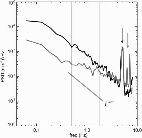
Velocity turbulence measurements were recorded at a single-point with a Nortek Vector acoustic velocimeter sampling at 16 Hz in 8,196-point bursts every 20 minutes. This instrument was mounted at mid-depth on a swivel-vane connection above the RDCP on the same taut mooring. The velocimetry-derived turbulent energy dissipation rate ε_v was resolved using the inertial dissipation method (IDM, Drennan et al. 1996) applied to the region of the 1024 point power spectral density distributions above the noise floor. The timeseries segments were despiked and then a section of the spectrum was extracted based on the criteria that a) the least squares fit (LSF) residual was smaller than a critical value and b) the spectral slope was close to the theoretical −5/3 slope associated with a Kolmogorov inertial subrange of turbulence. Considering example spectra (Figure 4), a compromise based on the LSF and slope criteria (Figure 8) indicated a band between 0.5 Hz and 1.6 Hz provided the most resolvable slope regions whilst still avoiding the noise floor, mooring vibrations and low-frequency variability. Surface waves were very short wave length and so did not penetrate sufficiently deep to influence the mooring instruments. The example spectra (Figure 4) show good (black), and poor (grey), quality realisations.

Figure 4. Example Vector power spectral density (PSD) distribution showing a spectrum which met the acceptance criteria (black) and a rejected spectrum which did not (grey). Mooring vibration modes are identified with arrows. The two vertical lines show the frequency range over which the f^−5/3 (grey solid sloping line) energy distribution is estimated. The dotted lines are the best-fit slope for the selected spectra.

Profiled data

Water column profiles were recorded from the RV Kaharoa, moored approximately 500 m to the NE of the mooring (Figure 2C), to provide a platform for profiling. Scalar conductivity-temperature-depth (CTD) profile data were recorded with a Seabird Electronics SBE19+ instrument lowered from the vessel. This sampled on average at 20 cm vertical resolution.

Forty two microstructure profiles were recorded over a single tidal cycle with a VMP500 (Vertical Microstructure Profiler–Rockland Oceanographic, Canada) profiler. The VMP500 free-fall loose-tether profiling instrument supported two shear probes, two fast thermistors, accelerometers and a Seabird Electronics (SBE) conductivity and temperature sensor pair. Each microstructure profile is effectively an instantaneous snap-shot. The profiles were recorded in batches of six profiles at a time, a few minutes apart. A disadvantage of the shear profiler approach in the present shallow water situation is the limit to vertical coverage. It requires a depth of approximately 5 m for the instrument to reach the terminal speed (c. 0.65 m s⁻¹) where the sensors operate effectively, and so the upper part of the water column is not sampled. Furthermore, in order to not damage the sensors on the muddy channel bed, the profile was stopped before encountering the floor of the channel. It did however provide a vertical context for the fixed point Vector turbulent energy dissipation rates.

The shear-derived dissipation rate of turbulent kinetic energy ε_s (m² s⁻³ or W kg⁻¹) was estimated using (Lueck 2005) where ν is kinematic viscosity and u_z is the local shear (vertical gradient of horizontal velocity). This was calculated (e.g. Lueck 2005) by first removing the accelerometer-inferred noise from the shear spectrum, replacing this with a modelled spectrum and then integrating across wavenumber (assuming a frozen-field hypothesis).

All profilers were recorded relative to the surface. The velocimeter was tethered to the bed but due to mooring motion this was not at a fixed height and so, as with the profilers, was treated as being relative to the surface via its pressure sensor. Only the RDCP data were recorded in the reference datum of the bed, and were therefore interpolated onto a depth ordinate for comparison.

Results

Meteorological conditions were average for February for the region with typically consistent fine conditions, whereby diurnal winds reached 7–10 m s⁻¹ during the day and air temperatures ranged between 13 and 23°C. A sea breeze effect was apparent from vessel-mounted meteorological instruments. Wind directions were highly variable due to the complex orography and it was not uncommon to observe, from the same vantage point, white-capped waves moving in different directions in different parts of the channel.

Acoustic current profiler (RDCP)

The tidal elevation during the observation period ranged over 2 m (velocimeter pressure, Figure 5A), 15% larger than at the entrance to the Sound. The main features of the RDCP current profiles were reasonably regular through the tidal cycles (Figure 5). The major principal axis of the current (see inset in Figure 6) was 12 degrees counter-clockwise from true north and, with only a 2% effect, we consider north-south to be equivalent to the along-channel component. The east-west across-channel tidal component was smaller, allowing the majority of the analyses to be carried out on the north-south (i.e. along-channel) component (Figure 5B). At the mooring location, the northward ebb phase had about 20% stronger peak currents than the southward rising flood flow, with the fastest ebb flows seen to be around 0.7 m s⁻¹ (Figure 5A,B). Possibly, this was due to horizontal heterogeneity whereby the centre of the ebb and flood flows take different pathways. However, a similar ebb dominance, but at a different location further out into Pelorus Sound, was observed by Sutton and Hadfield (1997). As well as sustaining lower overall speeds, the southward (flood) flow exhibited greater variability in flow speed as well. The transient bump in pressure (Figure 5A) is most likely a knock-down effect whereby the mooring is pushed over slightly at high flow but only observed on the ebb tide. The combined velocimeter pressure and RDCP velocity (Figure 5A,B) shows the maximum flow speed on the falling tide (ebb) arrives essentially right on mid-water. The maximum speed on the flood phase however is broad and falls a little after mid-water.

Figure 5. A 2-day section of the RDCP velocity data showing A, depth at the mooring and the north-south current component at mid-depth (northward is ebb, positive and shaded), B, the north-south velocity distribution (m s⁻¹) as a function of height above bed and C, velocity shear (s⁻¹). The Vector is located at height 17 m.

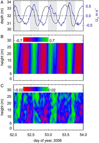
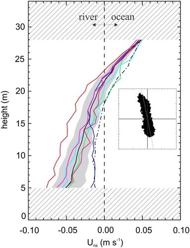
Figure 6. Tidal-cycle temporal averages of tidal principal axis along-channel (quasi-north-south) velocity profile from the RDCP. Hatched sections are outside the RDCP sample volume. The data were divided into 12.4 hour sections and time-averaged. The solid black line is the overall average (to the nearest 12.4 hours) and the shaded zone is the total average +/− the standard deviation at each depth. The dash-dot line is the cross-channel equivalent (arranged so that positive is westward so as to correspond to ebb). The averages were conducted over exact semidiurnal tidal periods. The scale of the inset box (showing north-south vs east west flow samples) is +/− 1 ms⁻¹ in both axes.

Examination of large scale vertical velocity shear (Sh_A) using the RDCP data (i.e. not the microscale shear) effectively removes the vertically averaged velocity and so reveals the subtleties in the flow structure (Figure 5C). The velocity shear in this panel is at the RDCP bin scale (1 m) rather than microstructure shear. The bands of positive shear extend over the entire sampled water column. The clearest signal in the shear is that on the switch from ebb to flood where there is a full-depth gradient in velocity. This drives the straining of the density structure. The reverse situation on the return from flood to ebb has no such clear signal. As the tide moved to flood conditions, there was an immediate switch in velocity gradient so that the lower half of the water column was flowing faster than that above (Figure 5C). In addition, there were several shear events deeper in the water column of opposite sign during the southward flood flow events. These perturbations reached one third of the absolute flow speed and a shear of 0.02 s⁻¹. While this generally fits the paradigm of an estuary with a strong freshwater inflow, it is not clear that this was the cause of the observed velocity profile as the riverine inflow at the time of sampling was low (Figure 3).

The temporal averages of velocity across a tidal cycle recorded with the RDCP (Figure 6) suggest that there is estuarine circulation with stronger northward (positive) outflow in the channel in the surface water, countered by a net inflow near the bed. This is consistent with the fresher surface water, being replaced with more dense, saline water near the bed. At the measurement location there is a bias to stronger inflow although this is possibly partly due to more of the outflow being outside the RDCP vertical sampling volume. It is also affected by there being far more variability near the bed where the standard deviation is around 30% of the mean. This deviation collapses to effectively zero in the upper-most measurements. The equivalent cross-channel residual (Figure 6) is less than a third of the along-channel residual near the bed but is comparable in the upper part of the water column implying a modest secondary cross channel flows persist.

Water column stratification

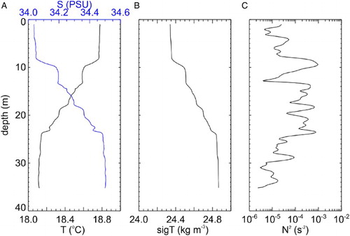
The density stratification exhibited a total top-to-bottom/surface-to-bed density difference of roughly 0.5 kg m⁻³. Sutton and Hadfield (1997) observed that top-bottom density differences could be 10 times this after periods of rain in Beatrix Bay 30 km further out into the Sound. At the time of the present measurements, the water column was stably stratified in both temperature and salinity, with the latter making the greatest contribution to stratification (Figure 7). The density structure was characterised by benthic and surface quasi-homogeneous boundary-layers separated by an internal stratified interfacial layer. These layers were roughly of equal thickness at the start of the detailed observation period at high tide (Figure 7). The buoyancy frequency squared (Figure 7C) reached nearly 10⁻³ s⁻² at the interfaces of the density structure (Figure 7B). There was substantial variation in the density structure throughout the tidal cycle with reduced surface layer salinity at the end of the ebb tide. At this time fine-scale instabilities were observed at both interfaces. The fact that such events are apparent in the relatively coarse SBE19+ CTD data suggests they were substantial. The buoyancy frequencies resolved from the CTD data allow the baroclinic Rossby radius of deformation L_R to be calculated and so the influence of rotational processes can be gauged. This is given by L_R = NH/(πf) where H is the water column depth and f is the Coriolis frequency (c. 10⁻⁴). Using N of 0.01 (Figure 7B) implies that L_R = 1200 m which is essentially the same as the channel width at the point the observations were recorded. This suggests rotation will be a secondary but measurable influence.

Figure 7. Example CTD profile showing A, temperature and salinity; B, density (sigma t = density – 1000 at atmospheric pressure); and C, buoyancy frequency squared.

Turbulence

The turbulence timeseries data recorded using the Vector velocimeter were of high quality with regard to backscatter and correlation signals (Figure 8A) with only moderate tilting effects due to mooring ‘knock-down’. Absolute velocities resolved using the Vector velocimeter compared very well with the RDCP bin at the Vector depth, reaching 0.7 m s⁻¹ (Figure 8B). Isolation from surface gravity wave smearing effects meant that spectral analysis typically resolved a clear inertial subrange. Spectra with slopes identified as being sufficiently close to f^−5/3 were collated and analysed (Figure 8C) to provide a timeseries of velocimeter-based dissipation rate (ε_v) estimates (Figure 8D) such that individual realisations of ε_v ranged between 4 × 10⁻⁸ and 2 × 10⁻⁶ m² s⁻³.

Figure 8. Velocimeter data showing A, total pitch and roll and velocity estimate correlation as a percentage (corr pcnt); and B, absolute velocity (the grey line is the equivalent depth bin of the RDCP). The ε_v estimate fitting parameters are shown in C, as slope marked as circles (shaded area as threshold) and the least squares fit (LSF) residual (line, with dashed line as threshold). Good fits are solid circles. Panel D, shows velocimeter depth pressure along with all the ε_v estimates. Good fits are solid circles.

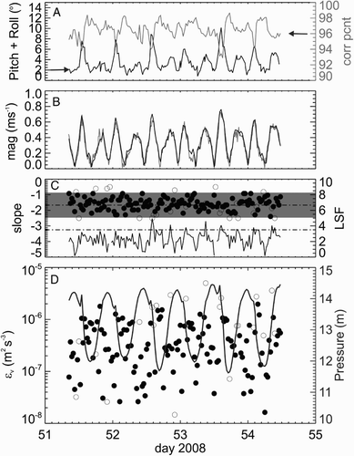
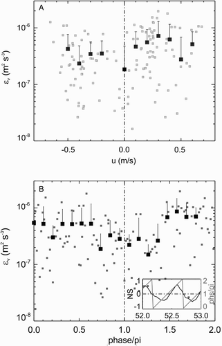
These estimates for ε were aggregated over tidal velocity and phase (Figure 9) so that the bin-averages were between 2 × 10⁻⁷ and 6 × 10⁻⁷ m² s⁻³. It was apparent that, at the depth of the sensor at least, there was no direct correlation between velocity and ε_v (Figure 9), although the zero flow speed did occur at the same time as the lowest dissipation rate estimate (2 × 10⁻⁷ and 6 × 10⁻⁷ m² s⁻³). Some structure did emerge when considering the dissipation rate from the velocimeter in relation to the tidal velocity phase (Figure 9B). With zero phase as selected here commencing on the slack-water prior to flood, the minimum dissipation rate occurs a little after slack water prior to ebb, which itself is a little later than the 180 phase shift would imply. The turbulent dissipation rate increases to the maximum for the entire cycle around mid-ebb. From the mid-depth location perspective, the ebb tide was slightly more dissipative than flood tide, contrary to the strain-induced periodic stratification model suggested by Simpson et al. (1990). A similar pattern was observed by Peters and Bokhorst (2000) during spring tides on the Hudson River.

Figure 9. Velocimeter estimates of ε_v A, as function of north-south velocity (measured values as open squares and solid squares are binned values with 0.1 m s⁻¹ bins, error-bars shows + 1 standard deviation) so that positive u is the ebb tide (Northward flowing); and B, as function of tidal speed phase (radian) where 0-π is the flood, and π−2π is the ebb. The inset shows the phase construction.

The shear microstructure profiler provides a vertical context for the estimates of dissipation rate (ε_s) which ranged between 5 × 10⁻⁸ and 5 × 10⁻⁶ m² s⁻³ with a dependence on the tidal phase and isopycnal displacements (Figure 10). The tidal flows associated with the 2 m tidal range are sufficient to drive internal dynamics that have apparent vertical isopycnal excursions, as observed in one location, comparable to half the water depth. The selected isopycnals in Figure 10 show the intermediate layer is compressed to almost zero thickness just after high tide but then rapidly expands to almost fill the water column prior to low tide. This later period also sees the strongest changes in dissipation rate. During the start of falling tide (day 52.54) the majority of the water column exhibits low ε_s, whereas 2 hours later (day 52.62) with the expansion of this middle ‘layer’ the near-bed ε_s reached 10⁻⁵ m² s⁻³–the highest recorded during the sampling. This coincided with maximum water speed (Figure 4A) and a decrease in salinity throughout the water column.

Figure 10. A, Density profiles from the CTD offset by 0.5 kg m⁻³ (scale bar top right) captured at times marked by dashed lines connecting the two panels. The dashed lines show the respective 24.5 kg m⁻³ value. B, Energy dissipation rate ε_s (m² s⁻³) from the shear SMS profiles along with the pressure at the velocimeter showing tidal height variation, and the shaded band is between two isopycnals (24.5 and 24.6 kg m⁻³) estimated from the VMP’s temperature and conductivity sensors (not the CTD, so the shaded band in panel B doesn’t exactly match the CTD in panel A).

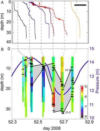
Low tide (day 52.7) saw the dissipation rate drop back to ε_s = 10⁻⁶ m² s⁻³ reasonably consistently throughout the sampled water column (Figure 10B). This reduction continued during the rising phase with a minimum in ε_s in the mid-depth region. During the ebb phase of the tide the density showed a strong decrease of 0.75 kg m⁻³ in a thin 5 m layer near the surface.

The shear microstructure (SMS) profiles were from similar times to the CTD profiles in Figure 10A, and while the finescale SMS data (Figure 11B) naturally contain more variability than the slower response CTD measurements the data coverage did not include the near-surface water column. The Richardson number (Ri_gr), quantifies shear-driven instability and was determined by interpolating the RDCP and CTD gradients to a consistent vertical basis (Figure 11B). The lower Ri_gr regions (i.e. prone to instability and mixing) were typically observed in the boundary layers. The mid-water column, experienced values of Ri_gr of 20 or more (so <−2 in the inverted Ri_gr shown in Figure 11B), indicative of stable conditions.

Figure 11. A, depth of velocimeter (add 17 m for full water depth) and depth-averaged northward-southward (northward = ebb) current from the RDCP. B, Offset density profiles as per Figure 10A where the scale bar is 0.5 kg m⁻³ and with Ri_gr superimposed (plotted in inverse form log₁₀[1/(4Ri_gr)] so that Ri_gr = 0.25 is 0, and reduced stability is greater in value, i.e. bright spots = ‘mixing’). The profiles are alternately solid and dashed to aid in identification.

Discussion

Turbulence energetics in context

These data capture a tidally varying stratification, turbulent eddy dissipation, and shear in the lower part of the water column. There is broadly consistent behaviour in the velocimeter-derived mid-depth dissipation rate ε_v over the tidal cycle. The ε_v are reasonably low through late rising tide and then increase dramatically by an order of magnitude at the same time as the velocity maximum causes the vector mooring to tilt slightly (time 52.57). Turbulence dissipation rate levels drop right after low tide.

The Hikapu channel can be considered ‘short’ compared to some other studies (see channel length L_c in Table 1), with the length being only a few multiples of the width. This may complicate the flow in that any vertical-axis eddy-structure introduced at the entrance to the channel will appear at the measurement site. Considering other comparable studies (Table 1) it is clear that this is not uncommon. Potentially, headland eddies (Edwards et al. 2004) generate structure seen at frequencies higher than the driving semi-diurnal frequency. In the present study there was a local peak in the velocity energy structure at 10 cpd which might well relate to eddy periods. The effect of these can be seen in the variability in velocity in Figure 5A. A width-scale transverse internal seiche mode within the channel would have a timescale of around 3 hours and is therefore potentially a driver for energy at 10 cpd.

In calculating the timescale ratio M for Hikapu Reach, we use C_d = 0.0025 (Nikora et al. 2002) for the inner Marlborough Sounds since the bed is typically smooth. The tidal flow duration relative to time for mixing of the water column, indicates that Mc. 0.7 (U_T = 0.5 m s⁻¹, N = 0.01 s⁻¹ and H = 32 m). This suggests that the system does not mix within a single phase of the tidal cycle, consistent with the observations. Sutton and Hadfield (1997) observed the annual cycle of buoyancy frequency N and determined that N at this time was likely at a mid-point in the annual cycle so the calculated value for M should be considered to be influenced in a similar pattern.

With regard to other systems, the Hudson River region has probably been the most heavily sampled estuarine system with the present focus but has no particular isolated channel sub-section. San Francisco Bay experiments (Suisan, but not the close-by channel data of Meeker) also fall centrally into the distribution of bulk properties and does have channel sections. Of the more idiosyncratic systems, the Hopkins estuary in Australia is by far the outlier. It is difficult to categorise as it is effectively a tidal surface layer moving over a quasi-stagnant pool and sustains a very sharp interface (N²  = 0.2 s⁻²). The present dataset from Hikapu Reach is the closest to the Cordova Channel in British Columbia based on geometry, tides and the presence of a channel section. The well-sampled Cordova site appears to be the least stable from a bulk perspective although the location is located within the wider estuarine conditions of the Strait of Georgia. The Meeker system near Berkeley, California, is comparable to Hopkins in terms of stability but the much smaller depth and high level of turbulence results in it being an extreme condition.

Geyer and MacCready (2014) developed a regime diagram casting M against a riverine Froude number that balances river flow speed against longwave speed in the estuary. Interestingly, this diagram indicates the Froude number is typically well below unity by orders of magnitude (i.e. subcritical). It is not clear that this would always apply here because the present situation is so close to the small, fast flowing Pelorus River mouth. This flow is likely to be highly variable and possibly supercritical following floods, or at least have a transitional river mouth-estuary confluence mixing region similar to that seen in some river-fjord interface zones (e.g. O’Callaghan & Stevens 2015).

The horizontal gradient of density, required to describe the horizontal buoyancy variation in the Si balance, is poorly constrained by the present data set. A Si value of unity requires a variation in density of 0.1 kg m⁻³ per km. Given that the Pelorus system goes from riverine to oceanic in 55 km (i.e. 4–5 times this gradient) this would suggest that Sic. 5–10 and thus indicates that strain will support stratification adequately through the entire tidal cycle. This is supported by the observations.

Comparison between turbulence measurement techniques

The turbulence estimation techniques revealed a high level of variability in magnitude and vertical extent of mixing. The velocimeter-based IDM approach had the best coverage in time but is confined to a single depth. Conversely, the SMS approach provided reasonable coverage in time over modest vertical coverage (Figure 10). The inverted gradient Richardson number profiles (Figure 11B) suggest that the primary period of low stability and likely mixing is deeper in the water column around time 52.45–52.5 on the growth phase of the ebb tide. The only strong turbulence signal in the upper water column was just after maximum ebb.

A comparison between the dissipation rate estimates from the velocimeter (ε_v) and shear microstructure (ε_s) gave the closest results, in terms of lines of best-fit, at around 10⁻⁷ m² s⁻³ (Figure 12, although it must be noted that the direct instrumental comparisons were not so good at this point). The slope (in log-log space) of the direct comparison is 0.45 such that the shear value underestimated the velocimeter value. However, arguably this is biased by an outlying set of estimates (shaded square in Figure 12). The slope after removing this point is 0.75. Despite the relatively few shear microstructure data points, the comparison indicates the two approaches resolved essentially the same trend in the same order of magnitude. Further experimentation with more data and perhaps improved co-location would enhance this comparison. In addition, it would be useful to augment this experiment with estimates from the ADCP variance-based approach (Stacey et al. 1999; Orton & Visbeck 2009), which while it does suffer from lack of full depth of coverage, does have good temporal coverage and, like the velocimeter IDM approach, can operate in stand-alone fashion. However, both moored approaches require additional sensors to capture the stratification and no technique adequately resolves close to the surface, which is important for quantifying air-sea exchange (Orton et al. 2010).

Figure 12. Comparison of dissipation rate estimates from velocimeter (ε_v) and shear microstructure (ε_s). Individual realisations of microstructure ε_s from the velocimeter depth are circles and the binned averages are the squares. The dashed line is the one-to-one fit. Fit A is through all the binned means and line B is excluding the shaded outlier as discussed in the text.

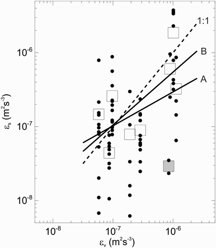
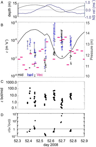
Figure 13. A, Depth of velocimeter (add 17 m for full water depth) and depth-averaged northward-southward (northward = ebb) current from the RDCP. B, Dissipation rate (ϵ) where the velocimeter estimates are pink horizontal lines extending over the duration of the data burst. The shear SMS estimates are shown as vertical lines bracketing the two shear probe estimates (black at depth of Vector velocimeter, blue at deepest point in profile). The velocimeter pressure is retained for reference. C, Ratio of SMS dissipation rates from deepest to velocimeter-depth bins. D, Average of ratio of ε_s to law of the wall dissipation for deeper half of water column.

The relative strengths of internal shear-driven and bed-driven turbulence

While the gradient Richardson number provides an overarching parameter for categorising stratified turbulence per se, mixing in tidal channels is likely to be primarily boundary-driven. These data illustrate how the Ri_gr fails to be a useful predictor of strong turbulent mixing as the largest dissipation rates are on the ebb (Figure 13B) whereas the Ri_gr (Figure 11B) had some low values on the ebb but more consistent values (high in terms of the inverted form as plotted) around high tide. It also demonstrates that the interplay between bed and internally-driven dissipation rate which, when viewed as a ratio (Figure 13B), is everywhere above unity except during the falling flood tide. The mid-depth velocimeter will capture bed-driven turbulence if the boundary influence penetrates sufficiently high into the water column. The mixing near the bed is over two orders of magnitude greater than at intermediate depth during maximum flow on the ebb. While the present work has an intra-tidal focus compared to Orton and Visbeck’s (2009) much longer and wider focus, the general results compare sufficiently well with the paradigm described by Geyer and MacCready’s (2014) review.

The bottom-mid-depth comparison of ε_s suggests that the turbulence, as identified by dissipation rate, is generally from bed generation (Figure 13C). However, comparison with a law of the wall expectation suggests there is more complexity than direct correspondence. The ratio of the observed ε to the law of the wall inferred dissipation rate profile (u³ _*/(kz)) is a measure of how substantial the internally generated turbulence is. The vertical averages of this (Figure 13D) were less than expected by the law of the wall turbulence representation during maximum ebb. This is most likely to be affected by the stratification although there could be some influence of the drag coefficient whereby u*c. . In addition, the comparison was influenced by slack water when the benthic shear stress denominator is low, so that the ratio is high.

While the focus above compared the bed-driven to internal mixing, Orton et al. (2010) showed that wind stirring controlled the turbulence in a surface layer, dominating the effect of the tide. Evidence of wind-driven turbulence in the surface layer may be seen in Figure 10 at day 52.7 when the top 5 m of the water surface becomes well mixed following an increase of wind speed to 10 m s⁻¹. This would depend on the relative strengths of the tides and wind as well as the stratification. However, it demonstrates that quantification of riverine influences on estuaries like Pelorus (and the Hudson where Orton et al. 2010 worked) need to consider factors beyond simply tides. This is highly relevant to estuarine/coastal air-sea gas exchange problems (Bauer et al. 2013).

Implications for exchange and dilution in the regional context

The Marlborough Sounds region is subject to substantial aquaculture activity, primarily shellfish (where nutrients are removed from the system) but also some fish cage activity (generating highly focused point-sources of nutrients). Quantifying the spreading and dilution of these perturbations on the natural system is important in terms of assessing the viability of such activities (Proctor & Hadfield 1998). Critically, with a tidal channel being located close to the riverine source, this initial mixing zone has an effect on the stratification throughout the sound.

Freshwater fronts have been observed with propagation speeds of 0.9 m s⁻¹ (Carter 1976) which would suggest a time to traverse the 4 km long section of a little over an hour. It suggests that a version of M, but with the tidal timescale replaced with a traversal timescale, would be useful. Or alternatively a separate scale ratio, C_r, could be considered that compared the tidal excursion to the channel length so that:where L_c is the length of the channel. A channel ratio C_r much greater than one suggests that the channel is short and so mixing within the channel, as defined by M, does not dominate. With L_c in Hikapu Reach being around 4 km and U_T = 0.7 m s⁻¹, this suggests a ratio of c. 4. This is likely transitional so that the mixing conditions identified by the basin scales Si and M are useful but likely not fully-developed as the turbulence will not have time to affect the full water column.

A key theme of interest is the effect of the channel on frontal structure during substantial freshwater events. With the varying mixing in the channel over the tidal cycle, there would be some influence on the sharpness of the front depending on the phase of the tide when the front entered the channel. The channel has the potential to act as a pre-conditioner for spreading into the rest of the Sound. However, given that the bed-driven mixing does not homogenise the water column under the current low river flow conditions, this effect may not be particularly strong here. Many estuaries have tidal channels within their basin, both in New Zealand (e.g. Raglan Harbour, McKergow et al. 2010) and internationally, that might experience a difference in the balance of transport and mixing.

Considering the channel length ratio C_r in Table 1, there is a separation introduced here between systems with an identifiable mid-estuary channel and those where the whole estuary system is considered. Either way, the channel length ratio is never greater than 10 or less than 0.1 putting most systems in a situation where advection is not the dominant factor (at either extreme). The well-defined channels are on the upper side of the scale with the present system being around 4 and other isolated sections (Cordova and Suisun) even higher.

The tidal mixing described here can be viewed in the context of similar datasets from embayments within the same system. Observations from Beatrix and Crail Bays (Stevens 2003, 2010, respectively) show more diverse (and typically slower) velocity structure. Despite being an embayment well off the main axis of the Sound and 25 km further towards the ocean, Crail Bay for example, exhibited a range of turbulent dissipation rates comparable with that found here. This was due to the lower stability in Crail Bay with a density stratification which was a factor of 2–3 lower than the Hikapu Reach observations. The stronger salinity stratification at Hikapu Reach results from the close proximity to the riverine freshwater sources.

This work suggests that the mixing that takes place in the Hikapu Reach is insufficient to homogenise any salinity signatures. Further study should examine the relative roles of tidal channels and embayments, and the influence of the timescale for mixing within the channel section, in controlling fluxes and residence times in complex estuaries. It would appear that future work should seek to better understand a modified M that incorporated duration of passage through a tidal channel.

Acknowledgements

The authors wish to thank Cliff Law for his support of this work. Warren Thompson, Matt Evans, Craig Stewart and Brett Grant are thanked for their assistance in the field, as are the Captain and crew of the RV Kaharoa.

Associate Editor: Associate Professor Conrad Pilditch.

Disclosure statement

No potential conflict of interest was reported by the authors.

ORCID

CL Stevens http://orcid.org/0000-0002-4730-6985

Additional information

Funding

The work was supported by the Ocean-Atmosphere Programme funded by NIWA Core Funding.

References

- Appell GF, Bass PD, Metcalf M. 1991. Acoustic Doppler current profiler performance in near surface and bottom boundaries. IEEE J Oceanic Eng. 16:390–396. doi: 10.1109/48.90903
- Bauer JE, Cai WJ, Raymond PA, Bianchi TS, Hopkinson CS, Regnier PA. 2013. The changing carbon cycle of the coastal ocean. Nature. 504:61–70. doi: 10.1038/nature12857
- Carter L. 1976. Seston transport and deposition in Pelorus Sound, South Island, New Zealand. New Zeal J Mar Freshwat Res. 10:263–282. doi: 10.1080/00288330.1976.9515612
- Drennan WM, Donelan MA, Terray EA, Katsaros KB. 1996. Oceanic turbulence dissipation measurements in SWADE. J Phys Oceanogr. 26:808–815. doi: 10.1175/1520-0485(1996)026<0808:OTDMIS>2.0.CO;2
- Edwards K, MacCready P, Moum J, Pawlak G, Klymak J, Perlin A. 2004. Form drag and mixing due to tidal flow past a sharp point. J Phys Oceanogr. 34:1297–1312. doi: 10.1175/1520-0485(2004)034<1297:FDAMDT>2.0.CO;2
- Geyer WR, MacCready P. 2014. The estuarine circulation. Annu Rev Fluid Mech. 46:175–197. doi: 10.1146/annurev-fluid-010313-141302
- Geyer WR, Scully ME, Ralston DK. 2008. Quantifying vertical mixing in estuaries. Env Fluid Mech. 8:495–509. doi: 10.1007/s10652-008-9107-2
- Grant HL, Stewart RW, Moilliet A. 1962. Turbulence spectra from a tidal channel. J Fluid Mech. 12:241–263. doi: 10.1017/S002211206200018X
- Heath RA. 1976. Tidal variability of flow and water properties in Pelorus Sound, South Island, New Zealand. New Zeal J Mar Freshwat Res. 10:283–300. doi: 10.1080/00288330.1976.9515613
- Li M, Gargett A, Denman K. 2000. What determines seasonal and interannual variability of phytoplankton and zooplankton in strongly estuarine systems? Estuar Coast Shelf Sci. 50:467–488. doi: 10.1006/ecss.2000.0593
- Lu Y, Lueck RG, Huang D. 2000. Turbulence characteristics in a tidal channel. J Phys Oceanogr. 30:855–867. doi: 10.1175/1520-0485(2000)030<0855:TCIATC>2.0.CO;2
- Lueck R. 2005. Horizontal and vertical turbulence profilers. In: Baumert HZ, Simpson JH, Sundermann J, editors. Marine turbulence: theories, observations and models. Cambridge, UK: Cambridge University Press; p. 89–100.
- McKergow LA, Pritchard M, Elliott AH, Duncan MJ, Senior AK. 2010. Storm fine sediment flux from catchment to estuary, Waitetuna-Raglan Harbour, New Zealand. New Zeal J Mar Freshwat Res. 44:53–76. doi: 10.1080/00288331003721471
- Nikora V, Goring D, Ross A. 2002. The structure and dynamics of the thin near-bed layer in a complex marine environment: a case study in Beatrix Bay, New Zealand. Estuar Coast Shelf Sci. 54(5):915–926. doi: 10.1006/ecss.2001.0865
- O’Callaghan JM, Pattiaratchi CB, Hamilton DP. 2010. The role of intratidal oscillations in sediment resuspension in a diurnal, partially mixed estuary. J Geophys Res. 115:C07018. doi:10.1029/2009JC005760.
- O’Callaghan JM, Stevens CL. 2015. Transient river flow into a fjord and its control of plume energy partitioning. J Geophys Res. (Oceans). 120. doi:10.1002/2015JC010721.
- Orton PM, Visbeck M. 2009. Variability of internally generated turbulence in an estuary, from 100 days of continuous observations. Cont. Shelf Res. 29:61–77. doi: 10.1016/j.csr.2007.07.008
- Orton PM, Zappa CJ, McGillis WR. 2010. Tidal and atmospheric influences on near-surface turbulence in an estuary. J Geophys Res. 115:C12029. doi:10.1029/2010JC006312.
- Peters H. 2003. Broadly distributed and locally enhanced turbulent mixing in a tidal estuary. J Phys Oc. 33:1967–1977. doi: 10.1175/1520-0485(2003)033<1967:BDALET>2.0.CO;2
- Peters H, Bokhorst R. 2000. Microstructure observations of turbulent mixing in a partially mixed estuary. Part I: Dissipation rate. J. Phys Oceanogr. 30:1232–1244. doi: 10.1175/1520-0485(2000)030<1232:MOOTMI>2.0.CO;2
- Proctor R, Hadfield M. 1998. Numerical investigation into the effect of freshwater inputs on the circulation in Pelorus Sound, New Zealand. New Zeal J Mar Freshwat Res. 32:467–482. doi: 10.1080/00288330.1998.9516837
- Ralston DK, Stacey MT. 2007. Tidal and meteorological forcing of sediment transport in tributary mudflat channels. Cont. Shelf Res. 27:1510–1527. doi: 10.1016/j.csr.2007.01.010
- Rippeth TP, Williams E, Simpson JH. 2002. Reynolds stress and turbulent energy production in a tidal channel. J Phys Oc. 32:1242–1251. doi: 10.1175/1520-0485(2002)032<1242:RSATEP>2.0.CO;2
- Sharples J, Coates MJ, Sherwood JE. 2003. Quantifying turbulent mixing and oxygen fluxes in a Mediterranean-type, microtidal estuary. Ocean Dynam. 53:126–136. doi: 10.1007/s10236-003-0037-8
- Simpson JH, Brown J, Matthews J, Allen G. 1990. Tidal straining, density currents, and stirring in the control of estuarine stratification. Estuaries. 13:125–132. doi: 10.2307/1351581
- Simpson JH, Williams E, Brasseur LH, Brubaker JM. 2005. The impact of tidal straining on the cycle of turbulence in a partially stratified estuary. Cont Shelf Res. 25:51–64. doi: 10.1016/j.csr.2004.08.003
- Stacey MT, Monismith SG, Burau JR. 1999. Observations of turbulence in a partially stratified estuary. J Phys Oceanogr. 29:1950–1970. doi: 10.1175/1520-0485(1999)029<1950:OOTIAP>2.0.CO;2
- Stevens C. 2003. Turbulence in an estuarine embayment: observations from Beatrix Bay, New Zealand. J Geophys Res. 108. doi:10.1029/2001JC001221.
- Stevens C. 2010. Short-term dispersion and turbulence in a complex-shaped estuarine embayment. Cont Shelf Res. 30:393–402. doi:10.1016/j.csr.2009.12.011.
- Sutton P, Hadfield M. 1997. Aspects of the hydrodynamics of Beatrix Bay and Pelorus Sound, New Zealand. New Zeal J Mar Freshwat Res. 31:271–279. doi: 10.1080/00288330.1997.9516764
- Walters RA, Goring DG, Bell RG. 2001. Ocean tides around New Zealand. New Zeal J Mar Freshwat Res. 35:567–579. doi: 10.1080/00288330.2001.9517023
- Wild-Allen K, Skerratt J, Whitehead J, Rizwi F, Parslow J. 2013. Mechanisms driving estuarine water quality: a 3D biogeochemical model for informed management. Estuar Coast Shelf Sci. 135:33–45. doi: 10.1016/j.ecss.2013.04.009
- Zeldis JR, Hadfield MG, Booker DJ. 2013. Influence of climate on Pelorus Sound mussel aquaculture yields: predictive models and underlying mechanisms. Aquacult Env Interac. 4:1–15. doi: 10.3354/aei00066